HAL Id: hal-01457737
https://hal.archives-ouvertes.fr/hal-01457737
Submitted on 27 Oct 2020
HAL is a multi-disciplinary open access
archive for the deposit and dissemination of
sci-entific research documents, whether they are
pub-lished or not. The documents may come from
teaching and research institutions in France or
abroad, or from public or private research centers.
L’archive ouverte pluridisciplinaire HAL, est
destinée au dépôt et à la diffusion de documents
scientifiques de niveau recherche, publiés ou non,
émanant des établissements d’enseignement et de
recherche français ou étrangers, des laboratoires
publics ou privés.
climate reconstructions under changing atmospheric
CO2 concentrations
E. Boucher, Joel Guiot, Christine Hatté, V. Daux, P-A Danis, Philippe
Dussouillez
To cite this version:
E. Boucher, Joel Guiot, Christine Hatté, V. Daux, P-A Danis, et al.. An inverse modeling approach
for tree-ring-based climate reconstructions under changing atmospheric CO2 concentrations.
Bio-geosciences, European Geosciences Union, 2014, 11 (12), pp.3245-3258. �10.5194/bg-11-3245-2014�.
�hal-01457737�
www.biogeosciences.net/11/3245/2014/ doi:10.5194/bg-11-3245-2014
© Author(s) 2014. CC Attribution 3.0 License.
An inverse modeling approach for tree-ring-based climate
reconstructions under changing atmospheric CO
2
concentrations
É. Boucher1, J. Guiot2, C. Hatté3, V. Daux3, P.-A. Danis4, and P. Dussouillez2
1Dept of Geography and GEOTOP, Université du Québec à Montréal, Montréal, Canada
2CEREGE, Aix-Marseille Université CNRS UMR7330, Europôle de l’Arbois, 13545 Aix-en-Provence, France
3LSCE-IPSL, UMR CEA-CNRS-UVSQ 8212, 12, L’Orme des Merisiers, 91191 Gif-sur-Yvette, France
4Onema-Irstea Hydro-écologie Plans d’Eau, 3275 Route de Cézanne, CS 40061, 13182 Aix-en-Provence, France
Correspondence to: É. Boucher ([email protected])
Received: 24 October 2013 – Published in Biogeosciences Discuss.: 28 November 2013 Revised: 17 April 2014 – Accepted: 24 April 2014 – Published: 17 June 2014
Abstract. Over the last decades, dendroclimatologists have
relied upon linear transfer functions to reconstruct historical climate. Transfer functions need to be calibrated using recent
data from periods where CO2 concentrations reached
un-precedented levels (near 400 ppm – parts per million). Based on these transfer functions, dendroclimatologists must then
reconstruct a different past, a past where CO2
concentra-tions were far below 300 ppm. However, relying upon trans-fer functions calibrated in this way may introduce an unantic-ipated bias in the reconstruction of past climate, particularly
if CO2has had a noticeable impact on tree growth and
wa-ter use efficiency since the beginning of the industrial era. As an alternative to the transfer function approach, we run the MAIDENiso ecophysiological model in an inverse mode
to link together climatic variables, atmospheric CO2
concen-trations and tree growth parameters. Our approach endeavors to find the optimal combination of meteorological conditions that best simulate observed tree ring patterns. We test our approach in the Fontainebleau Forest (France). By
compar-ing two different CO2 scenarios, we present evidence that
increasing CO2concentrations have had a slight, yet
signif-icant, effect on the reconstruction results. We demonstrate
that realistic CO2concentrations need to be inputted in the
inversion so that observed increasing trends in summer
tem-perature are adequately reconstructed. Fixing CO2
concen-trations at preindustrial levels (280 ppm) results in undesir-able compensation effects that force the inversion algorithm to propose climatic values that lie outside from the bounds of observed climatic variability. Ultimately, the inversion ap-proach has several advantages over traditional transfer
func-tion approaches, most notably its ability to separate climatic
effects from CO2 imprints on tree growth. Therefore, our
method produces reconstructions that are less biased by an-thropogenic greenhouse gas emissions and that are based on sound ecophysiological knowledge.
1 Introduction
With climatic change and rising CO2 concentrations, the
need to place recent trends in a multisecular perspective has led to an unprecedented expansion of the field of pa-leoclimatology. Tree rings have played a central role in that development, offering the possibility to reconstruct var-ious climatic fields at high temporal resolution (annual to intra-annual) (e.g., Fritts, 1976; Schweingruber, 1996) and over large areas (regional (e.g., Cook et al., 2004), hemi-spheric (e.g., Esper et al., 2002; Briffa et al., 1998a; Mann et al., 1999) or global (e.g., Mann et al., 2008)). To per-form such reconstructions, dendrochronologists have typi-cally relied upon various black-box approaches (also called transfer functions) (Fritts, 1976) that approximate relation-ships between tree rings and climate by a time-invariant func-tion. However, evidence for nonstationarity and divergence in the biological response to climate have called into ques-tion the transfer funcques-tion approach (Vaganov et al., 2006). Time-varying tree-ring-to-climate responses may have vari-ous origins (D’Arrigo et al., 2008): thresholded, complex and nonlinear responses, changes in resources and nutrient avail-ability (Reich and Hobbie, 2013; Silva and Anand, 2013),
alteration of climate–growth relationships by CO2and sus-tained changes in water-table levels. If these phenomena are not accounted for in the reconstruction model, discrepancies between real and reconstructed paleoclimatic variability can be expected (Briffa et al., 1998b).
Since carbon dioxide is well mixed and homogeneously distributed throughout Earth’s atmosphere (Myhre et al.,
1998), CO2 might be one of the most widespread sources
of divergence, yet its biological impact on climate-to-tree-growth relationships remains imprecise (D’Arrigo et al.,
2008). Since the beginning of the industrial period, CO2
con-centrations have increased by about 150 ppm (parts per mil-lion), reaching 400 ppm in 2013 (Tans and Keeling, 2013). Whether or not this increase has had a significant effect on tree growth however remains vigorously debated. On one hand, several studies that aimed at detecting and attribut-ing the various signals contained in tree rattribut-ings argued against a possible long-term fertilization effect (e.g., (Gedalof and Berg, 2010; Silva et al., 2010; Girardin et al., 2011)). On the other hand, a whole set of empirical experiments (see reviews by Norby et al. (1999), Norby et al. (2005) and more recently the landmark paper by Keenan et al. (2013)), though
con-ducted on smaller timescales, have concluded that CO2has
had important effects on tree productivity and water use ef-ficiency. However, eddy-covariance measurements cannot be directly compared with tree ring series to precise the role of
CO2 on overall productivity and water use efficiency, since
the former does not allow discriminating between trees, un-derstory vegetation, and soil respiration/evapotranspiration. From a paleoclimatological perspective, this debate is funda-mental. If tree ring chronologies have been imprinted by a
strong CO2signal since the late industrial period (LaMarche
et al., 1984), the appropriateness of transfer models needs to be called into question, as it cannot be assumed that recent tree-ring-to-climate relationships reflect those of the
prein-dustrial period, a period where CO2 concentrations were
lower than at present.
To circumvent the possible biases caused by divergent re-lationships, several alternatives exist, most of which make use of extensive process-based modeling. Data-assimilation approaches such as the one proposed by Goose et al. (2010) aim at constraining climate models in order to identify plau-sible and coherent climatic scenarios that match the varia-tions of natural proxies. Data-assimilation techniques allow testing various forcing scenarios, but in the case of tree rings, the linkages between climate simulations and proxies remain imprecise as signal and noise components cannot be clearly distinguished. In other fields of paleoclimatology, several au-thors have put forward the idea that deterministic models can be reversed so that the set of rules and mathematical equa-tions representing the many processes that occur in ecosys-tems can be used in an inverse mode to retrieve probabilistic estimates for input meteorological conditions (Chuine et al., 2004; Hughes and Ammann, 2009; Guiot et al., 2009, 2000; de Cortázar-Atauri et al., 2010; Evans et al., 2013). This
ap-proach has been tested by Garreta et al. (2010) for pollen data, yet no dendroecological model was inverted to perform a reconstruction. Tolwinski-Ward et al. (2011) have recently accomplished a first step towards the reconstruction and used a simplified version of the Vaganov–Shashkin model (VS-lite) that mimics the principle of a limiting factor to simulate thresholded ring-width responses. However, while a simple water bucket model is efficient computationally, some of the most important ecophysiological processes responsible for tree growth in nature (e.g., stomatal conductance, photosyn-thesis, resource allocation and partitioning of carbon, reuse of the preceding year’s photosynthetates, etc.) are omitted, with uncertain consequences for the inversion. Additionally, in VS-lite, the focus is on a single proxy (ring widths) while it has been demonstrated that a multiproxy approach is the most efficient way to enhance long-term environmental sig-nals (McCarroll and Loader, 2004; Mann, 2002). Variables such as oxygen and carbon isotopes in tree-ring cellulose are now routinely measured; so inverse modeling approaches need to account for these proxies that may present comple-mentary signals and different sources of noise (McCarroll and Loader, 2004).
Here, we present a reconstruction performed from the in-version of the MAIDENiso model (Danis et al., 2012), an up-dated version of the MAIDEN model (Misson, 2004) that ac-counts for carbon and oxygen isotope fractionation. MAID-ENiso is a full ecophysiological model, meaning that the links between meteorological (input) variables and (output) tree ring variables (e.g tree ring widths, carbon and oxygen isotopes) are not empirically parametrized as in a regression, but explicitly represented as mathematical equations within the model. The main objective of this paper is to demonstrate the scientific and conceptual advantages that inverse den-droclimatological modeling may have for the study of past climates. With this objective in mind, we will address the following questions: (1) how good are the reconstructions performed from the inversion? (2) Are they better than tra-ditional transfer function techniques based, for example, on linear modeling? (3) Is the approach able to take into account
and eventually isolate the effect of CO2on tree ring growth
and thus attest of its impact on past climates reconstructed from tree ring series?
This paper will be divided in two parts. In the first part, we rapidly review the model’s capability as well as its parametrization. We then present our inversion approach ex-plicitly. In the second part, we apply the inversion technique to reconstruct past climatic variations in the Fontainebleau Forest (near Paris, France), where Danis et al. (2012) have recently calibrated the model.
2 MAIDENiso
MAIDENiso is a process-based, dendrogeochemical model that can simulate various tree growth parameters useful in
dendroecological analysis such as tree ring widths, δ18O and
δ13C of tree ring cellulose. Earlier versions of the model were
used to simulate tree growth in northern and southern France (Gaucherel et al., 2008; Misson et al., 2004), as well as Bel-gium (Misson, 2004). Recently, the model was completed by
Danis et al. (2012) to capture the main variations of δ18O
and δ13C of tree ring cellulose found in sessile oak
(Quer-cus petraea Matt.). In the forward mode, it uses relatively
simple meteorological inputs: daily precipitation (cm d−1),
minimum and maximum temperature (◦C). However, other
variables are also required (on a daily basis) such as
atmo-spheric concentration of CO2(ppm), the content of δ18O of
precipitation, and δ13C content in atmospheric CO2. Lastly,
a limited amount of parameters need to be found in the lit-erature or estimated directly from tree rings using optimiza-tion techniques (see Gaucherel et al. (2008) and Misson et al. (2004) for more explanations).
MAIDENiso captures and models site-specific phenologi-cal as well as meteorologiphenologi-cal controls on transpiration, stom-atal conductance, respiration and photosynthetic production. For an extensive review of the processes and how they are modeled, readers are referred to the original works by Mis-son (2004) and Danis et al. (2012). The algorithm includes several allocation rules that distribute biomass production, carbon and oxygen isotopes in various reservoirs such as leafs, bole, roots, and storage. From a dendroecological per-spective, bole is the most important reservoir, as it can be readily compared to standard tree ring measurements such
as tree ring widths, δ18O and δ13C. However, storage is
an-other important property of the model as it allows simulat-ing processes responsible for autocorrelation and persistence in tree growth parameters, therefore enabling the use of car-bohydrates to be passed to the next year of simulation. This aspect has important implications in ecology but also in pale-oclimatology. For example, in the case of the Fontainebleau Forest (described later) Danis et al. (2012) argued that an ad-equate modeling of storage reserves by MAIDENiso allowed for a proper simulation of the 1976 drought in that area. In the years following the drought, and in spite of the ameliora-tion of climatic condiameliora-tions, trees were unable to store a suffi-cient amount of reserves, which resulted in sustained growth reductions. From a paleoclimatological perspective, it is im-portant that the inversion distinguishes between climatic and storage-related effects. Otherwise, prolonged ecophysiologi-cal responses could be mistaken for persistent harsh climatic conditions.
3 MAIDENiso’s inversion procedure
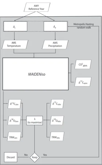
The inversion approach described here (Fig. 1) allows to retrieve paleoclimatic information from ecophysiological models. The method is presented with examples from the Fontainebleau Forest (France). First, it must be stated that inverse modeling procedures do not aim at finding a back-ward solution to the set of rules and equations that are im-plemented in a process-based model. Instead, inverse mod-eling approaches seek for the optimal combination of input data so that outputs (i.e., simulations) are as close as pos-sible to the observations. In the precise context of dendroe-cological modeling, inverting a model such as MAIDENiso implies finding the optimal combination of meteorological inputs that will best simulate tree ring parameters (tree ring
widths, δ18O and δ13C). Consequently, the model has to be
run repeatedly with different meteorological scenarios each time, preserving only the ones that simulate tree ring param-eters that resemble observations, and eliminating the rest.
So, at first glance, a contradiction seems to emerge: the model has to be run with meteorological data to produce tree ring simulations, but, in the case of a climate reconstruc-tion, it is precisely those conditions that are unknown. There-fore, the general strategy proposed here is to define, from the modern data set, a reference or average meteorological year (AMY) that will serve as a basis to produce alternative me-teorological scenarios (Fig. 1). Identifying the AMY ensures that a certain degree of temporal coherence exists in the rela-tionship between temperatures and precipitation. In the case of the Fontainebleau Forest, the meteorological data set orig-inally used by Danis et al. (2012) corresponds to the aver-age of two stations (Glandée at Villiers-en-Bière and Fais-sandière at Fontainebleau) located 10km north of the forest. From this data set and with a simple measure of euclidian distance, we identified 1984 as the year that is closest, in terms of average temperature and precipitation (spring and summer) to the 1953–2000 average (Fig. 2a, b). Figure 2c and d present temperature and precipitation variations that occurred in 1984 at Fontainebleau. The temperature curve presents a typical hyperbolic shape with an average
temper-ature of 10.2◦C. The precipitation series depicts
consider-able variability at the daily to monthly scales, with low sum-mer precipitation and precipitation peaks in June (4.5 cm) and September (3.8 cm), respectively, and with an average of 0.27 cm precipitation per day.
Once the AMY is identified, the next step is to find a way to modify it in order to produce alternative meteorological scenarios (AMS) that will be iteratively reinjected within MAIDENiso, through the undermentioned inversion algo-rithm. The strategy proposed here is to modify the AMY’s original temperature and precipitation series with constants (thereafter named deltas, or 1) that generate AMS. For each year simulated, we defined two different 1: one for
temper-ature (δτ) that is additive and a second for precipitation (δπ)
∆π ∆τ Discard Metropolis Hasting random walk MAIDENiso AMY Reference Year CO2 atm δ13Csim δ18Osim TRWsim Keep AMS Precipitation AMS Temperature δ13Catm δ13Cobs δ18Oobs TRWobs Yes No λ (to maximise)
Figure 1. MAIDENiso’s inversion flowchart. For each year
simu-lated, two 1 modify the AMY: one for temperature (δτ t) and one for
precipitation (δπ t). The resulting AMS is passed to MAIDENiso,
along with atmospheric CO2concentrations and atmospheric δ13C
to simulate tree growth parameters. Simulated tree growth is com-pared to observations, through the metric λ, which has to be maxi-mized (Eq. 1). The Metropolis–Hastings algorithm iteratively mod-ifies the value of δτand δπso that it converges towards stable states
(Eq. 2).
season, which is defined here as the period between early April (Julian day 91) and late October (Julian day 304). Fig-ure 2c and d present two alternative meteorological
scenar-ios computed from two different δτ and δπ values. In the
first scenario (red), δτ and δπ were assigned a value of 2,
meaning that all days are incremented positively by 2◦C, and
that all precipitation events, when they occur, are doubled in magnitude. In the second scenario (blue), we assigned values
of −2 and 0.5 to δτ and δπ, respectively. Therefore, 2◦were
subtracted to the temperature series and the daily amount of precipitation was halved during the growing season.
δτ and δπ were implemented so that the modifications of
meteorological conditions by the Metropolis–Hastings algo-rithm (described hereafter) are kept as simple and straight-forward as possible. However, the modifications themselves must be confined within bounds that respect the properties of local climatology in order to avoid generating implausi-ble meteorological conditions. Uniform priors are then set to
δτ and δπ, with values bounded between −5 and +5 for the
former and between 0.25 and 4 for the latter. Such values produce bounds that are larger than the modern (1950–2000) interannual meteorological variability, but were set uniform because we assumed to have no a priori knowledge on past fluctuations within these bounds. Moreover, Gaussian priors centered around AMY would give too much weight to the “normal” conditions and are likely to be incompatible with our wish to generate sufficiently different climatic conditions from the present ones.
The Metropolis–Hastings random walk algorithm (MHA) is used to estimate, for each year t of the reconstruction
the posterior probability distribution of δτ (t ) and δπ(t ). The
MHA is a Markov chain Monte Carlo (MCMC) procedure and therefore sample candidates produced within the chain depend only on the current sample value. The chain gresses towards a stable state by accepting or rejecting pro-posed samples. Concerning our application, the posterior
dis-tribution of δτ (t ) and δπ(t )corresponds to the distribution of
accepted values that best simulate tree ring parameters, at year t .
The MHA is extensively described in Hastings (1970); here, the most important principles will be presented and ex-emplified with our tree ring application (Fig. 1). For each meteorological year t to be reconstructed from tree ring
pa-rameters, let f (1t) be a target density that is proportional
to the desired probability distribution of 1 at year t, P (1t).
First, f (1t) executes a MAIDENiso run through which tree
ring parameters are simulated given input AMS. Then a met-ric λ (Fig. 1) needs to be maximized [−∞ → 0] and corre-spond to the negative squared distance between simulated (s) and real-world observations (o):
λt= −(δ13Ct (s)−δ13Ct (o))2−(δ18Ot (s)−δ18Ot (o))2 (1)
−(TRWt (s)−TRWt (o))2.
To calculate λ, all tree ring variables are transformed into dimensionless standardized scores. From there, the MHA
starts by defining current values for δτ t (i) and δπ t (i)
(here-after grouped into 1t (i)) that fall within the bounds of a
uni-form prior distribution q(1t|1t (i)). The algorithm then
de-fines a candidate set of deltas: 1∗t. The chain M walks
to-wards the next iteration, accepting or rejecting the candidate values according to the following rules:
M =
P (1t (i), 1∗t) if f (1t∗) ≥ f (1t (i);(accept 1∗t)
P (1t (i), 1∗t)α if f (1∗ t) < f (1t (i);(accept 1 ∗ t with α = ef (1∗ t)−f (1t (i)))
P (1t (i), 1t (i+1))(1 − α) if α < 1; (reject 1∗t with 1 − α).
0 100 200 300 0 5 10 20 Temperature (°C) 0 100 200 300 0 2 4 6 8
Julian days (ca 1984)
Precipitaion (cm) 0 100 200 300 0 100 200 300 15 16 17 18 19 20 1960 1970 1980 1990 2000 20 60 100 Temperature (°C) Years Precipitaion (cm) a) b) c) d)
Figure 2. Yearly and daily (1984) summer temperature and precipitation series for the Fontainebleau Forest. The left panel presents
temper-ature (a) and precipitation (b) series, with the AMY (1984) indicated by red squares. Average conditions are in dashed red. The right panel presents daily variations (in 1984) for temperature (c) and precipitation (d). Black curves represent observations in 1984 (AMY). The red curve corresponds to the AMS that results from the modification of the AMY by a δτ of 2 and a δπof 2. The blue curve represents an AMS
that originates from the modification of the AMY by a δτ of −2 and a δπof 0.5.
In other words, if f (1∗t) ≥ f (1t (i), then the candidate set
1∗t is more likely than the original set of deltas to produce
tree ring parameters that mimic those found in nature. In that
case, 1∗t is accepted with a probability of 1 and the
algo-rithm “walks” to the next iteration replacing 1t (i+1)by 1∗t.
In the case where f (1∗
t) < f (1t (i), there are two
possibili-ties. First, there is a chance equal to α that 1∗
t is accepted and
passed to the next iteration. Second, there is a 1-α chance that
1∗t is rejected and consequently, 1t (i) is maintained at the
next iteration. After a large number of iterations, the chain
M will tend to be proportional to P (1t) because the
algo-rithm will “intuitively” visit high-density regions more often than it does for low-density regions.
The inversion scheme presented earlier (Fig. 1) enables
sampling in the posterior distribution P (1t) one year at a
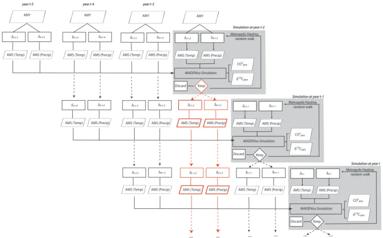
time. However, tree ring series usually present a certain de-gree of autocorrelation. Such a persistence may be caused by climatic variations, but may also result from persisting insuf-ficient carbon storage. Fortunately, MAIDENiso can account for storage and remobilization of carbon reserves within the tree, but to do so, it needs to simulate more than a single year at a time. In order to correctly model autocorrelation, we opted for a 4-year block simulation (Fig. 3). Thus, to
ob-tain a distribution for 1t, we fed MAIDENiso with 1t −1,
1t −2, and 1t −3, which are passed from the preceding
sim-ulations (dashed lines on Fig. 3). Hence, all four 1 respec-tively modify the AMY (year 1984) to produce 4-year-long daily temperature and precipitation series that are used by MAIDENiso. Accordingly, simulated tree ring series exhibit a 4-year dependance structure that should be similar to the
one observed in real world samples. Median δτ (t ) and δπ(t )
values are passed to the subsequent year and so forth (Fig. 3). It is important to underline that the optimization of the metric
λ(Eq. 1) by the MHA is exclusively performed for the last
year of the simulation, irrespective of the number of years included in the simulation.
4 Application of the inversion algorithm to the Fontainebleau Forest (France)
4.1 Tree ring data
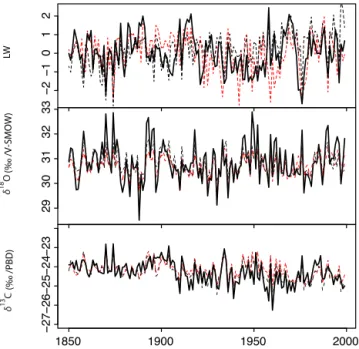
All tree ring data (Fig. 4) used for the inversion are late-wood measurements previously published by Etien et al. (2008). Thirty living, dominant oaks were sampled in the Fontainebleau Forest (two stations, N = 15/station). On each tree, three cores were sampled at 1.3 m height. Each series was measured and cross-dated by the phytoecology team of the National Institute of Agronomical Research (INRA, Nancy, France) using a master chronology constructed from more than 400 oaks sampled in the nearby area. The living tree chronology was standardized using the adaptive regional growth curve technique (Nicault et al., 2010) to produce an average chronology (Fig. 4a). Tree rings were then cut us-ing a scalpel to separate latewood from earlywood. Samples were pooled and then milled with an 80 µ sieve. α-cellulose was extracted using the Soxhlet method (Leavitt and Danzer, 1993). Isotopic compositions (Fig. 4b, c) were determined with a Carbo Erba elemental analyzer coupled to a Finnigan MAT252 mass spectrometer (at LSCE, Gif/Yvette, Fr).
Cor-rection of cellulose δ13C series for the Suess effect was not
AMY ∆π t-2 ∆τ t-2 Metropolis Hasting random walk MAIDENiso Simulation ∆π t-2 ∆τ t-2 ∆π t-3 ∆τ t-3 AMY ∆π t-3 ∆τ t-3 AMY ∆π t-4 ∆τ t-4 Discard ∆π t-1 ∆τ t-1 Keep Metropolis Hasting random walk MAIDENiso Simulation Discard Simulation at year t ∆π t-1 ∆τ t-1 ∆π t-2 ∆τ t-2 ∆τ t ∆π t Metropolis Hasting random walk MAIDENiso Simulation Discard Simulation at year t-1 Simulation at year t-2 CO2atm Keep Keep AMS (Precip)
AMS (Temp) AMS (Temp) AMS (Precip)
CO2atm δ13Catm δ13Catm δ13Catm CO2atm ∆π t-4 ∆τ t-4 AMY ∆π t-5 ∆τ t-5 ∆π t-3 ∆τ t-3 AMS (Precip)
AMS (Temp) AMS (Temp) AMS (Precip)
AMS (Precip)
AMS (Temp) AMS (Temp) AMS (Precip) AMS (Precip)
AMS (Temp) AMS (Temp) AMS (Precip)
AMS (Precip)
AMS (Temp) AMS (Temp) AMS (Precip) AMS (Precip)
AMS (Temp) AMS (Temp) AMS (Precip)
year t-4 year t-3 year t-5
... ... ... ... ... ...
Figure 3. Flowchart of the autocorrelation modeling. Each gray box corresponds to the inversion algorithm presented in Fig. 1. For each year twhere the inversion is conducted, AMS from the three preceding years is also given as input to MAIDENiso, so the simulation is performed on a total of 4 years (bold arrows). Once the best combination of 1 is found by the Metropolis–Hastings algorithm, the mean δ values are passed to the next iteration. An example is given by red dashed lines. 1s found for year t − 2 are also used to simulate t − 1 and t.
an input and the model directly yields depleted series com-parable to those found in tree rings.
The sensitivity of tree ring proxies to climate was exam-ined by Etien et al. (2008). Briefly, Fontainebleau’s oaks re-spond to both summer temperature and precipitation, how-ever at different levels (Table 1). Latewood widths respond positively to summer precipitation while the correlation with summer temperature is not significant (Etien et al., 2008). This feature was also highlighted by Kelly et al. (2002) and recalls that, in temperate areas, oak growth is mainly
con-trolled by moisture availability. δ13C and δ18O variability are
both positively correlated to summer temperature and neg-atively related to summer precipitation (Etien et al., 2008).
Correlations with δ18O are slightly stronger, but the fact that
both isotopic proxies are sensitive to the same climatic vari-able suggest that, at Fontainebleau, stomatal closure is an im-portant response mechanism to drought.
4.2 Atmospheric data
In addition to tree ring and meteorological data, three addi-tional variables were prescribed as inputs to MAIDENiso:
atmospheric CO2concentrations, atmospheric δ13C content
Table 1. Correlation between (left column) observed and
recon-structed summer climatic conditions at the Fontainebleau Forest for the 1960–2000 period and (right column) correlation between tree rings and observed climatic conditions.
Reconstructed vs. Tree rings vs. observed climate observed climate
Trec Prec LW δ13C δ18O
Tobs 0.53 −0.3 −0.11 0.42 0.47
Pobs −0.3 0.67 0.42 −0.51 −0.65
and δ18O of precipitation. CO2 concentrations and
atmo-spheric δ13C were both derived from published ice core data
and were scaled with observations at the nearest CO2records
(Gif-sur-Yvette, France) while δ18O of precipitation (δ18Op)
was estimated statistically:
– Atmospheric CO2 concentrations. We retained two
scenarios that will help us identify CO2 effects and
associated biases within the reconstruction (Fig. 5). The first scenario (“A1”) mimics the reality and
−2 −1 0 1 2 29 30 31 32 33 1850 1900 1950 2000 −27 −26 −25 −24 −23 LW (‰ /PBD) δ 13 C (‰ /V-SMOW) δ 18 O
Figure 4. Observed and simulated tree ring proxies. Black bold
lines represent observed latewood widths (LW), δ18O and δ13C of tree ring α cellulose. Black dotted lines correspond to the simula-tions performed from the A1 (increasing CO2) scenario, while red
dotted lines represent the A2 (stable CO2) scenario.
towards modern values. The nearest CO2 record
(Gif-sur-Yvette) covers the 2000–2007 period. Only the mean annual cycle was retained from that short se-ries and was superimposed over the long-term trend in
CO2concentrations extracted from ice cores (Robertson
et al., 2001). The latter reflects global rather than local
trends in CO2. Therefore, both series were combined
into a single one and simply extrapolated at the daily time step as in Danis et al. (2012). Scenario A1 was also shifted by +15 ppm by comparison to the ice core se-ries to take into account observable differences between the two series during their common period. The second scenario (“A2”) represents a fictive situation into which
CO2concentrations have remained stable (at
preindus-trial levels, i.e., 280 ppm) over the full reconstruction period.
– Atmospheric δ13C content. Atmospheric δ13C data (Fig. 5) was retrieved from published ice core se-ries (Francey et al., 1999) and covers the full recon-struction period. Modern annual cycles were extracted from the Schauinsland data set (Black Forest, Germany) (Schmidt et al., 2003; Danis et al., 2012) that extends
back to ca. 1976. As for CO2trends, the Schauinsland
annual cycle was superimposed over the long-term trend extracted from the ice core series. The resulting series was shifted by 1 ‰ towards lighter ratios to match val-ues observed during the common period at Schauins-land.
Figure 5. Daily atmospheric CO2(a) and δ13C (b) data used in the
inversion. The A1 (black) scenario is a realistic one while scenario A2 (red) describes a hypothetical case where CO2concentrations
have remained at preindustrial (1850) levels.
– δ18O of precipitation. In MAIDENiso, δ18Op is
mod-eled statistically using linear regressions, with daily temperature and precipitation used as regressors (Da-nis et al., 2012). Regression parameters were
cali-brated using 42 years of δ18Op (dependant variable),
temperature and precipitation data extracted from the REMO(REgional MOdel)iso mesoscale climate model (Sturm et al., 2005). The regression equation was di-rectly incorporated into MAIDENiso’s code so that the
modeling of δ18Opcould be achieved at the daily time
step. Such parameters are site-specific.
4.3 Method of inversion-run details
In this study, a Metropolis–Hastings analysis were performed
using the R statistical software (RCore Team, 2012), most
particularly through themetrop( )function of themcmc
package (Geyer and Johnson, 2012). For each year t sim-ulated by the MHA, 500 burn-in samples were generated. Also, to ensure that the chain M is stable and composed only of successively uncorrelated and independent candidates, we
picked only one 1t candidate at each 100 accepted samples.
In total, we sampled 1000 candidate values for 1t. We
fi-nally verified the chain convergence by checking that the lag-1 correlation between successive candidate values remained below 0.35.
5 Results and discussion
Here we present a paleoclimatic reconstruction for the Fontainebleau Forest area, based on the inversion of the MAIDENiso model. The reconstruction extends back to ca. 1850 and focuses on summer (JJA) temperature and
precip-itation. The A1 CO2scenario is used, unless the contrary is
5.1 How good is the reconstruction performed from the inversion?
5.1.1 1960–1999 period
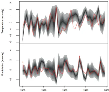
A comparison between reconstructed and observed summer climatic conditions is presented in Fig. 6 for the 1960–1999 period. The visual correspondence between both variables is fairly good, but slightly better for precipitation, both in terms of high-frequency and low-frequency variability. Re-constructed temperatures correlate well (r = 0.53) with ob-servations (Table 1, left column), but precipitation correlates even better (r = 0.67). As is the case for observed chronolo-gies (Table 1, right column) the temperature signal is weaker than the precipitation signal. In other words, the climatic sig-nal recorded by trees seems to be well extracted by our recon-struction. Moreover, as the model was already parametrized by Misson (2004) for tree rings and by Danis et al. (2012) for C and O isotopic fractionation, we argue that this climate re-construction is coherent with the main ecophysiological pro-cesses that govern tree growth at Fontainebleau.
In the present simulation, a single δτ (t )and δτ (t )value now
modifies the AMY to generate AMS but, ultimately, the com-parison is made only for the summer period, owing to the fact that all proxies were measured on latewood. Consequently, all AMY are modified identically between day 91 and day 304, with no distinction between spring and summer condi-tions. Accordingly, by increasing the number of parameters to be estimated one would certainly augment the resolution of the ecophysiological modeling, therefore allowing sea-sonal reconstructions to be performed. Seasea-sonal integration would enable the temporal integration of spring, summer and autumn growth processes and would yield even more sound reconstructions. Paleotemperature modeling would also cer-tainly benefit from such an approach because even more important for tree growth than absolute temperatures is the length of the growing season. For instance no parameters modify the length of the growing season, which is fixed to exactly 214 days. Further modeling efforts will be invested in order to increase the number of parameters to take into ac-count varying growing season length as well as seasonal dif-ferences between spring and summer. However, it remains to be demonstrated that the Metropolis–Hastings algorithm can still converge when the number of parameters is increased.
5.1.2 1850–1999 period
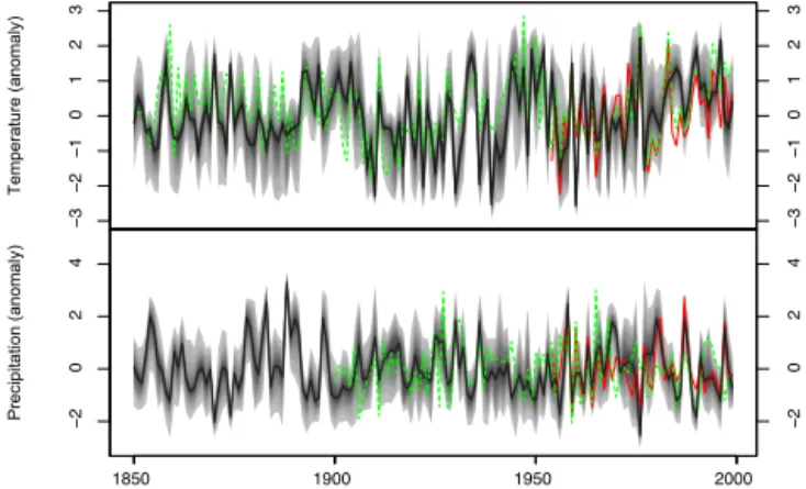
We extended the reconstruction back to AD 1850 and com-pared it to the Climate Research Unit (CRU) gridded tem-perature (CRUTEM4, Jones et al., 2012) and precipitation (Hulme et al., 1998) reconstructions (Fig. 7). The general agreement between both series is fairly good, with, again, a clear visual correspondence in the high- and low-frequency domains. The correlations with the CRU data are 0.51 and 0.40, respectively, for temperature and precipitation (n = 100
Figure 6. Comparison with modern climatological records (1960–
1999). Median reconstructed values correspond to the black curve, observations are in red. The quantiles between 2.5 and 97.5 fall within the gray shading.
for precipitation and n = 150 for temperature). The temper-ature reconstruction seems to be in phase with the CRU data and the correlation is similar to that calculated for the 1960– 1999 period. (Fisher r to z score = −0.15, p > 0.05). There is, however, a clear drop in the strength of the correlation for the precipitation (Fisher r to z score = 2, p < 0.05). While this drop could be interpreted as a flaw of the method, some other aspects must be considered. First, CRU data correlates poorly with precipitation at Fontainebleau over the 1960– 1999 period (r = 0.37), so there is no reason to assume that both series did correlate well in the past. Second, it is clear from the visual examination of both curves that low frequen-cies are well reconstructed. Such low frequenfrequen-cies may relate to the regional trend. However, high-frequency variations of precipitation are difficult to interpolate at the local scale, es-pecially in the Paris area where a temperate-oceanic climate dominates, with an important influence of convective precip-itation during the summer. This kind of precipprecip-itation may be hard to interpolate and, therefore, divergence can be expected with observations.
5.2 Does the reconstruction perform better than a linear transfer function?
Inversions were compared to the reconstructions obtained from calibrating transfer functions (multiple linear regres-sion) of the 1960–1999 period (Fig. 8). Although both tech-niques produce temperature and precipitation reconstructions that correlate well with one another, (r = 0.74 and 0.84, re-spectively), several differences need to be underlined. At first, a simple comparison of the variance for the pre-1950 and post-1950 periods shows that the transfer function leads
−3 −2 −1 0 1 2 3 −3 −2 −1 0 1 2 3 1850 1900 1950 2000 −2 0 2 4 −2 0 2 4 Temperature (anomaly) Precipitation (anomaly)
Figure 7. Summer temperature and precipitation reconstructions
back to ca. 1850. Reconstructed climatic conditions (black) are compared to the CRU (green) data during the common period. Ob-servations during the 1960–1999 period are in red. The quantiles between 2.5 and 97.5 fall within the gray shading.
to an underestimation of the variance of temperatures for the last 50 years. Taking the CRU (temperature) variance as a ref-erence for the pre-1950 period (0.9), the variance obtained by inversion is 0.91 and the transfer function produces a com-parable series (variance of 0.89). However, for the 1950– 2000 period, the CRU variance augments to 1.16. The in-version follows that trend (post-1950 variance of 1.12) while the transfer function does not and the variance remains low (0.81) after 1950. This is a very important point, as variance losses and underestimation have plagued the transfer func-tion approach over the last decade (Bürger, 2007) and may suggest that model inversions have a slight advantage over transfer functions from this point of view. For precipitation, the two methods produce series with comparable variances for both pre-1950 (0.90 ± 0.1) and 1950–2000 periods. Nev-ertheless, the transfer function methods creates a slight but significant (p < 0.01, n = 150) positive trend in the amount of summer precipitation. Such a trend leads to an underesti-mation of summer precipitation before 1900 and to a slight overestimation from 1950 onward. Such a trend does not ex-ist either in the inversion or in the CRU precipitation series over the last century (p > 0.05).
In addition to reproducing variance and trends that bet-ter characbet-terize Fontainebleau’s climate variability since AD 1850, the inversion approach seems to have other conceptual advantages. By contrast to traditional transfer functions, no calibration is required, except for the initial parametrization of the ecophysiological model (here, MAIDENiso). Conse-quently, we expect the method to be more adaptable to the modeling of nonstationary tree-ring-to-climate relationships. The inversion procedure also builds on sound ecophysiolog-ical knowledge and therefore the links between climate and tree growth are not reduced to a set of calibrated parameters, but are modeled with regards to the complexity and multi-plicity of processes that control vegetation growth. From a
−3 −2 −1 0 1 2 3 −3 −2 −1 0 1 2 3 1850 1900 1950 2000 −2 0 2 4 1850 1900 1950 2000 −2 0 2 4 Temperature (anomaly) Precipitation (anomaly)
Figure 8. Comparison between two reconstruction techniques: the
inversion of MAIDENiso (black) and the transfer function (dashed blue) calibrated for the 1960–1999 period.
modeling perspective, it is clear that each and every improve-ment made within the plant ecophysiology science commu-nity and implemented in deterministic models will directly translate to better reconstruction performances, and a greater adaptability of the model to a wide range of environments.
5.3 Is the reconstruction affected by changes in atmospheric CO2concentrations?
MAIDENiso is an ecophysiological model that simulates tree growth parameters, given atmospheric inputs such as
concen-trations in CO2and δ13C. Therefore, the model can be used
as a testbed to evaluate the impact, among other things, of
CO2 increases on the reconstruction. As mentioned earlier,
we performed two reconstructions, each forced with a
differ-ent CO2scenario (Fig. 5): scenario A1, which corresponds to
the typical anthropogenically modified curve; and A2, which
represents the nonanthropogenic curve (CO2remains stable).
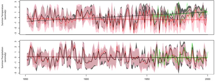
The A1 and A2 simulations yield divergent temperature reconstructions (Fig. 9). Both reconstructions correlate well with one another (r = 0.75 for temperature), implying that high-frequency variations are well reconstructed using both
CO2 scenarios. However, the series exhibit different
long-term trends. Temperatures reconstructed using the A1 sce-nario show a clear rise towards warmer conditions (a trend that is also observed in instrumental climatic series) while temperatures reconstructed using the A2 scenario slightly de-creased over time. Contrastingly, from the point of view of precipitation, the A1 and the A2 scenarios produced com-parable reconstructions at both high and low frequencies (r = 0.87).
Our results suggest that the inversion must be forced by
a realistic and increasing CO2 scenario (e.g., A1) to
-3 -2 -1 0 1 2 3 yr[-1] -3 -2 -1 0 1 2 3 Summer T emper atur e (anomaly) Summer P recipita tion (anomaly) 1850 1900 1950 2000
Figure 9. Summer temperature and precipitation reconstructions at Fontainebleau, France, obtained from the inversion of MAIDENiso.
Black curves and associated 95 % uncertainty range are median reconstructed values obtained when the inversion is constrained by realistic, increasing CO2data. The red curve and associated 95 % confidence intervals are median reconstructed values obtained when the inversion is
forced when CO2is fixed at preindustrial levels. Observed climate variability (1953–1999) is in dashed green. Linear lines with corresponding
colors were added to each series to evaluate multidecadal trends in reconstructed and observed climates.
This is because, at least at the Fontainebleau Forest, MAID-ENiso is able to balance the interplay between climate,
at-mospheric CO2concentrations, tree growth and isotope
frac-tionation, even when the interaction between these variables is not stationary through time. As a consequence, without
in-putting a realistic CO2 scenario to the inversion, the MHA
compensates by altering climate 1s in order to bring AMS outside from the bounds of observed variability and converge towards tree ring simulations that match with observations. The A2 reconstruction perfectly exemplifies this compen-sation phenomenon. When the inversion is forced by fixed,
preindustrial CO2concentrations, stomata remain open in
or-der to maximize carbon gains and simulate growth variations in a way that mimics observed tree ring series (i.e., measured from oak trees that grew in a CO2-enriched atmosphere). However, with stomata wide open, evapotranspiration rates increase accordingly and reconstructed temperature needs to drop significantly (Fig. 9) in order to reduce water losses at the leaf surface. It is important to recall that this compensa-tion mechanism originates from the fact that, no matter which
CO2scenario is chosen for the inversion, the MHA
systemat-ically “walks” towards the best way to modify climate inputs in order to keep λ as close to zero as possible. Ultimately, we could verify that, because of this compensation mechanism, simulated values for each tree ring proxy and for each sce-nario are strongly related to the original observations (Fig. 4, dashed lines).
The impact of CO2on the inversion needs to be discussed
in light of the mechanisms that govern CO2 exchanges at
the leaf–atmosphere interface. In MAIDENiso, stomatal con-ductance is modeled using the Ball et al. (1987) model, later modified by Leuning (1995), which is based on the early works of Wong et al. (1979). The Ball–Berry–Leuning
model expresses stomatal conductance as a function of
rela-tive humidity, photosynthesis and CO2concentrations at the
leaf surface. The equation however implies a nearly
con-stant ratio of internal (Ci) to atmospheric (Ca) CO2
concen-trations, which is maintained stable through stomatal aper-ture and closure. A direct consequence of the Ball–Berry–
Leuning model is a quasi-parallel response of internal (Ci)
to increasing CO2(Ca). For that reason, its applicability to
very high CO2concentrations (e.g., 700–800 ppm), without
accounting for acclimation mechanisms such as those men-tioned in Drake et al. (1997) (decrease in Rubisco, augmen-tation of carbohydrate solubility, increases in light use ef-ficiency, lower rates of dark respiration or nitrogen limita-tion (Berninger et al., 2004)) is queslimita-tionable. Our results suggest that the Ball–Berry–Leuning model might however
be appropriate for the range of CO2concentrations that
pre-vailed since (and even before) the preindustrial era. A corol-lary interpretation is that acclimation mechanisms must not have had a large influence over the last 150 years, at least in the Fontainebleau Forest’s context. Otherwise, the inver-sion would not have converged towards realistic climate sce-narios when forced by the A1 scenario. These findings ul-timately support the conclusions of Medlyn et al. (1999), which underly that in several environments, acclimation pro-cesses have not completely overridden the net carbon gains
related to CO2.
One of the strengths of our study is that the inversion of MAIDENiso is constrained by multiple proxies simul-taneously, rather than by a single one, therefore better re-flecting the array of physiological processes that govern tree growth. This is a very important point, especially in a con-text where the inversion is used to attest of the impact of CO2 on tree-ring-based climatic reconstructions. It is well known
that each proxy responds differently to rising CO2 concen-trations, each with its own strengths and source of bias. For example, tree ring widths potentially record changes in tree productivity, but low-frequency growth trends attributable to
rising CO2concentrations might be removed by
standardiza-tion (Melvin and Briffa, 2008; Cecile et al., 2013), in which case the inversion algorithm (like any other reconstruction method) would converge towards unrealistic trends that are
exempt of any CO2imprint. Similarly, it has been argued by
Silva and Horwath (2013) that, due to an artifact of
calcu-lation, δ13C chronologies might systematically overestimate
the response of carbon isotopes to rising CO2
concentra-tions, therefore creating artificial increases in reconstructed water use efficiency. However, as mentioned by McCarroll and Loader (2004) and also by Silva and Horwath (2013) for
the particular case of CO2effects, the solution might lie in
the use of multiple proxies, as it is proposed here. Although we cannot ignore the possible source of bias associated with each proxy, our approach certainly enables the simulation of all three proxies (from reconstructed climate) in a way that mimics real world observations (Fig. 4). Indeed, a large
num-ber of climatic and CO2combinations can explain variations
in each proxy individually, but a much smaller range of com-binations can explain covariations consistent with all three proxies. At the Fontainebleau site, it was previously shown by Etien et al. (2008) that stomatal conductance has a dras-tic importance on the overall growth, as evidenced by
nega-tive latewood width responses and covarying δ13C and δ18O.
In such water-sensitive environments, tree rings are
particu-larly responsive to CO2effects (Knapp et al., 2001; Owensby
et al., 1999; Huang et al., 2007), therefore reinforcing the
in-dispensable role of CO2on tree growth and isotope
fraction-ation at our site and, indirectly, attesting of the necessity to
include realistic CO2scenarios to produce unbiased climatic
reconstructions.
Ultimately, these results are appealing for the study of di-vergence in dendroclimatology (D’Arrigo et al., 2008) and suggest that the inversion of process-based dendroecological models is a suitable approach to reconstruct climate under
changing CO2 concentrations. As it was demonstrated
ear-lier, our analysis shows that tree-ring-to-climate relationships are significantly affected by changes in atmospheric CO2 concentrations. Failing to include a realistic atmospheric
CO2scenario triggers an undesirable climatic compensation
effect that forces the inversion to diverge from a realistic cli-matic reconstruction. Of course, the quality of the inversion will always be dependent on the quality of tree ring series used as reference. In this regard, the development of novel “signal free” standardization techniques (e.g., Melvin and Briffa (2008) or Cecile et al. (2013)) will help constrain the inversion with tree ring chronologies that contain as little bias and/or noise as possible. In addition, from an ecophysiolog-ical modeling point of view, the amelioration of equations and rules implemented within ecophysiological models from both field and experimental studies will contribute to expand
the applicability of the approach to a variety of environments and species. Finally, the improvement of random-walk algo-rithms and the design of better parametrization strategies will directly translate into more robust and more precise recon-structions.
6 Conclusions
In this study, we demonstrated that the MAIDENiso eco-physiological model can be used to perform paleoclimatic reconstructions that take into account the effect of
anthro-pogenic CO2 concentrations on tree growth. We provided a
way to inverse that model through the use of a random-walk Metropolis–Hastings algorithm that iteratively converges to-wards the best combination of meteorological conditions to fit observations. The approach was exemplified in a recon-struction of past summer temperatures and precipitation at the Fontainebleau Forest (France). The novel reconstruction technique seems to perform well in that environment, and presents significant conceptual advantages compared to the regression technique. First, since the inversion is constrained by an ecophysiological model such as MAIDENiso, the
com-plex and nonlinear interactions between climate, CO2
con-centrations and tree growth are mechanistically determined, and not reduced to a set of calibration parameters. Second, an ecophysiological model such as MAIDENiso can account for the temporal dependance of tree-ring-to-climate
relation-ships on changing CO2concentrations. It is therefore an
ap-pealing and promising tool for the study in divergence in den-droclimatology and for the reconstruction of climate in the presence of nonstationary tree-ring-to-climate relationships.
Our study shows that atmospheric CO2 is an important
variable at the Fontainebleau Forest, and as a consequence, it is necessary to constrain the inversion with a realistic
CO2 scenario in order to perform reconstructions that
con-verge towards observed climate variability. Running the
in-version with CO2concentrations fixed at preindustrial levels
(280ppm) forces the model to propose climate values that are outside from the bounds of observed variability. In the Fontainebleau context, this compensation effect leads to the reconstruction of a colder climate. This compensation mech-anism can be explained by links and feedbacks that exist between climate, stomatal conductance and photosynthesis, all of which are represented by MAIDENiso under the form
of mechanistic equations. With lower atmospheric CO2
con-centrations, stomata need to remain wide open in order to maximize carbon gains and match real-world growth rates. However, by doing so, water losses by evapotranspiration and evaporation at the leaf surface also increase. So, in or-der to compensate for water losses, reconstructed tempera-tures need to be lower, a situation that ultimately minimizes evapotranspiration and evaporation fluxes.
This analysis remains a first step towards a more gener-alized, large-scale utilization of ecophysiological models in
dendroclimatology. As suggested by Tingley et al. (2012), process-based models such as MAIDENiso can link instru-mental and proxy observations in a framework that accounts for nonstationary and nonlinear relationships. Because of that particularity, their integration in a Bayesian hierarchical modeling is highly desirable and can improve the quality of climate-field reconstructions while opening up new and stim-ulating perspectives on the modeling of the spatiotemporal dependence between proxies and observations. In that con-text, our work supports the ideas developed by Tingley et al. (2012) and exemplifies a case where a mechanistic model actually integrates, within the reconstruction, nonstationary tree-ring-to-climate relationships and their dependance on
changing CO2concentrations. In years to come, the
perfor-mance of the process-based inversion approaches will likely increase, as a result of the amelioration of equations and rules implemented within ecophysiological models, the improve-ment of random-walk and inversion algorithms, and the de-sign of better parametrization strategies.
Acknowledgements. The first author sincerely thanks the Fonds de Recherche Nature et Technologies (FRQNT) for its financial support. This work is a contribution to the Labex OT-Med (ANR-11-LABEX-0061) funded by the Investissements d’Avenir, French Government program of the French National Research Agency (ANR) through the A∗Midex project (ANR-11-IDEX-0001-02). Financial support was also provided by the ARCHIVES project funded by the Natural Sciences and Engineering Research Council of Canada (NSERC) as part of a collaborative research and development grant with OURANOS and Hydro-Québec.
Edited by: V. Brovkin
References
Ball, J. T., Woodrow, I. E., and Berry, J. A.: A model predicting stomatal conductance and its contribution to the control of photo-synthesis under different environmental conditions, in: Progress in photosynthesis research, 221–224, Springer, 1987.
Berninger, F., Hari, P., Nikinmaa, E., Lindholm, M., and Meriläinen, J.: Use of modeled photosynthesis and decomposition to describe tree growth at the northern tree line, Tree Physiol., 24, 193–204, 2004.
Briffa, K., Jones, P., Schweingruber, F., and Osborn, T.: Influence of volcanic eruptions on Northern Hemisphere summer tempera-tures over the past 600 years, Nature, 393, 450–454, 1998a. Briffa, K., Schweingruber, F., Jones, P., Osborn, T., Harris, I.,
Shiy-atov, S., Vaganov, E., and Grudd, H.: Trees tell of past climates: but are they speaking less clearly today?, Philos. T. Roy. Soc. B, 353, 65–73, 1998b.
Bürger, G.: On the verification of climate reconstructions, Clim. Past, 3, 397–409, doi:10.5194/cp-3-397-2007, 2007.
Cecile, J., Pagnutti, C., and Anand, M.: A likelihood perspective on tree-ring standardization: eliminating modern sample bias, Clim. Past Discuss., 9, 4499–4551, doi:10.5194/cpd-9-4499-2013, 2013.
Chuine, I., Yiou, P., Viovy, N., Seguin, B., Daux, V., and Ladurie, E. L. R.: Historical phenology: grape ripening as a past climate indicator, Nature, 432, 289–290, 2004.
Cook, E., Woodhouse, C., Eakin, C., Meko, D., and Stahle, D.: Long-Term Aridity Changes in the Western United States, Sci-ence, 306, 1015–1018, 2004.
Danis, P.-A., Hatté, C., Misson, L., and Guiot, J.: MAIDENiso: a multiproxy biophysical model of tree-ring width and oxygen and carbon isotopes, Canadian J. Forest Res., 42, 1697–1713, 2012. D’Arrigo, R., Wilson, R., Liepert, B., and Cherubini, P.: On the
“di-vergence problem” in northern forests: a review of the tree-ring evidence and possible causes, Global Planet. Change, 60, 289– 305, 2008.
de Cortázar-Atauri, I. G., Daux, V., Garnier, E., Yiou, P., Viovy, N., Seguin, B., Boursiquot, J., Parker, A., Van Leeuwen, C., and Chuine, I.: Climate reconstructions from grape harvest dates: Methodology and uncertainties, The Holocene, 20, 599–608, 2010.
Drake, B. G., Gonzàlez-Meler, M. A., and Long, S. P.: More effi-cient plants: a consequence of rising atmospheric CO2?, Annu.
Rev. Plant Biol., 48, 609–639, 1997.
Esper, J., Cook, E., and Schweingruber, F.: Low-Frequency Signals in Long Tree-Ring Chronologies for Reconstructing Past Tem-perature Variability, Science, 295, 2250–2253, 2002.
Etien, N., Daux, V., Masson-Delmotte, V., Stievenard, M., Bernard, V., Durost, S., Guillemin, M. T., Mestre, O., and Pierre, M.: A bi-proxy reconstruction of Fontainebleau (France) growing sea-son temperature from A.D. 1596 to 2000, Clim. Past, 4, 91–106, doi:10.5194/cp-4-91-2008, 2008.
Evans, M. N., Tolwinski-Ward, S., Thompson, D., and Anchukaitis, K. J.: Applications of proxy system modeling in high resolution paleoclimatology, Quaternary Sci. Rev., 76, 16–28, 2013. Francey, R., Allison, C., Etheridge, D., Trudinger, C., Enting, I.,
Leuenberger, M., Langenfelds, R., Michel, E., and Steele, L.: A 1000-year high precision record of δ13C in atmospheric CO2, Tellus B, 51, 170–193, 1999.
Fritts, H.: Tree rings and climate, Elsevier, 1976.
Garreta, V., Miller, P. A., Guiot, J., Hély, C., Brewer, S., Sykes, M. T., and Litt, T.: A method for climate and vegetation recon-struction through the inversion of a dynamic vegetation model, Clim. Dynam., 35, 371–389, 2010.
Gaucherel, C., Campillo, F., Misson, L., Guiot, J., and Boreux, J.-J.: Parameterization of a process-based tree-growth model: compar-ison of optimization, MCMC and particle filtering algorithms, Environ. Model. Softw., 23, 1280–1288, 2008.
Gedalof, Z. and Berg, A. A.: Tree ring evidence for limited direct CO2 fertilization of forests over the 20th century, Global
Bio-geochem. Cy., 24, GB3027, doi:10.1029/2009GB003699, 2010. Geyer, C. J. and Johnson, L. T.: mcmc: Markov Chain Monte Carlo, http://CRAN.R-project.org/package=mcmc, r package version 0.9-1, 2012.
Girardin, M. P., Bernier, P. Y., Raulier, F., Tardif, J. C., Concia-tori, F., and Guo, X. J.: Testing for a CO2 fertilization effect
on growth of Canadian boreal forests, J. Geophys. Res.-Biogeo. (2005–2012), 116, G01012, doi:10.1029/2010JG001287, 2011. Goose, H., Crespin, E., De Montety, A., Mann, M., Renssen,
H., and Timmermann, A.: Reconstructing surface temperature changes over the past 600 years using climate model
simula-tions with data assimilation, J. Geophys. Res., 115, D09108, doi:10.1029/2009JD012737, 2010.
Guiot, J., Torre, F., Jolly, D., Peyron, O., Boreux, J.-J., and Ched-dadi, R.: Inverse vegetation modeling by Monte Carlo sampling to reconstruct palaeoclimates under changed precipitation sea-sonality and CO2 conditions: application to glacial climate in
Mediterranean region, Ecol. Model., 127, 119–140, 2000. Guiot, J., Wu, H. B., Garreta, V., Hatté, C., and Magny, M.: A
few prospective ideas on climate reconstruction: from a statisti-cal single proxy approach towards a multi-proxy and dynamistatisti-cal approach, Clim. Past, 5, 571–583, doi:10.5194/cp-5-571-2009, 2009.
Hastings, W. K.: Monte Carlo sampling methods using Markov chains and their applications, Biometrika, 57, 97–109, 1970. Huang, J.-G., Bergeron, Y., Denneler, B., Berninger, F., and Tardif,
J.: Response of forest trees to increased atmospheric CO2, Cr.
Rev. Plant Sci., 26, 265–283, 2007.
Hughes, M. and Ammann, C.: The future of the past – an earth system framework for high resolution paleoclimatology: edito-rial essay, Climatic Change, 94, 247–259, 2009.
Hulme, M., Osborn, T. J., and Johns, T. C.: Precipitation sensitivity to global warming: Comparison of observations with HadCM2 simulations, Geophys. Res. Lett., 25, 3379–3382, 1998. Jones, P., Lister, D., Osborn, T., Harpham, C., Salmon, M.,
and Morice, C.: Hemispheric and large-scale land-surface air temperature variations: An extensive revision and an update to 2010, J. Geophys. Res.-Atmos., 117, D05127, doi:10.1029/2011JD017139, 2012.
Keenan, T. F., Hollinger, D. Y., Bohrer, G., Dragoni, D., Munger, J. W., Schmid, H. P., and Richardson, A. D.: Increase in forest water-use efficiency as atmospheric carbon dioxide concentra-tions rise, Nature, 499, 324–327, 2013.
Kelly, P. M., Leuschner, H. H., Briffa, K. R., and Harris, I. C.: The climatic interpretation of pan-European signature years in oak ring-width series, The Holocene, 12, 689–694, 2002.
Knapp, P. A., Soulé, P. T., and Grissino-Mayer, H. D.: Detecting po-tential regional effects of increased atmospheric CO2on growth
rates of western juniper, Glob. Change Biol., 7, 903–917, 2001. LaMarche, V. C., Graybill, D. A., Fritts, H. C., and Rose, M. R.:
Increasing atmospheric carbon dioxide: tree ring evidence for growth enhancement in natural vegetation, Science, 225, 1019– 1021, 1984.
Leuning, R.: A critical appraisal of a combined stomatal-photosynthesis model for C3 plants, Plant Cell Environ., 18, 339–355, 1995.
Mann, M., Bradley, R., and Hughes, M.: Northern hemisphere tem-peratures during the past millennium: Inferences, uncertainties, and limitations, Geophys. Res. Lett, 26, 759–762, 1999. Mann, M. E.: The value of multiple proxies, Science, 297, 1481–
1482, 2002.
Mann, M. E., Zhang, Z., Hughes, M. K., Bradley, R. S., Miller, S. K., Rutherford, S., and Ni, F.: Proxy-based reconstructions of hemispheric and global surface temperature variations over the past two millennia, P. Natil. Acad. Sci., 105, 13252–13257, 2008.
McCarroll, D. and Loader, N. J.: Stable isotopes in tree rings, Qua-ternary Sci. Rev., 23, 771–801, 2004.
Medlyn, B., Badeck, F.-W., De Pury, D., Barton, C., Broadmeadow, M., Ceulemans, R., De Angelis, P., Forstreuter, M., Jach, M.,
Kellomäki, S., Laitat, E., Marek, M., Philippot, S., Rey, A., Strassemeyer, J., Laitinen, K., Liozon, R., Portier, B., Robertntz, P., Wang, K., and PG, J.: Effects of elevated [CO2] on photo-synthesis in European forest species: a meta-analysis of model parameters, Plant Cell Environ., 22, 1475–1495, 1999.
Melvin, T. M. and Briffa, K. R.: A “signal-free” approach to dendro-climatic standardisation, Dendrochronologia, 26, 71–86, 2008. Misson, L.: MAIDEN: a model for analyzing ecosystem processes
in dendroecology, Can. J. Forest Res., 34, 874–887, 2004. Misson, L., Rathgeber, C., and Guiot, J.: Dendroecological analysis
of climatic effects on Quercus petraea and Pinus halepensis radial growth using the process-based MAIDEN model, Can. J. Forest Res., 34, 888–898, 2004.
Myhre, G., Highwood, E. J., Shine, K. P., and Stordal, F.: New es-timates of radiative forcing due to well mixed greenhouse gases, Geophys. Res. Lett., 25, 2715–2718, 1998.
Nicault, A., Guiot, J., Edouard, J., and Brewer, S.: Preserving long-term fluctuations in standardisation of tree-ring series by the adaptative regional growth curve (ARGC), Dendrochronologia, 28, 1–12, 2010.
Norby, R. J., Wullschleger, S. D., Gunderson, C. A., Johnson, D. W., and Ceulemans, R.: Tree responses to rising CO2in field
experi-ments: implications for the future forest, Plant Cell Environ., 22, 683–714, 1999.
Norby, R. J., DeLucia, E. H., Gielen, B., Calfapietra, C., Giardina, C. P., King, J. S., Ledford, J., McCarthy, H. R., Moore, D. J., Ceulemans, R., et al.: Forest response to elevated CO2is
con-served across a broad range of productivity, P. Natl. Acad. Sci. USA, 102, 18052–18056, 2005.
Owensby, C. E., Ham, J., Knapp, A., Auen, L., et al.: Biomass pro-duction and species composition change in a tallgrass prairie ecosystem after long-term exposure to elevated atmospheric CO2, Glob. Change Biol., 5, 497–506, 1999.
R Core Team: R: A Language and Environment for Statistical Com-puting, R Foundation for Statistical ComCom-puting, Vienna, Austria, http://www.R-project.org/, ISBN 3-900051-07-0, 2012. Reich, P. B. and Hobbie, S. E.: Decade-long soil nitrogen constraint
on the CO2fertilization of plant biomass, Nat. Clim. Change, 3,
278–282, 2013.
Robertson, A., Overpeck, J., Rind, D., Mosley-Thompson, E., Zielinski, G., Lean, J., Koch, D., Penner, J., Tegen, I., and Healy, R.: Hypothesized climate forcing time series for the last 500 years, J. Geophys. Res.-Atmos., 106, 14783–14803, 2001. Schmidt, M., Graul, R., Sartorius, H., and Levin, I.: The
Schauins-land CO2record: 30 years of continental observations and their
implications for the variability of the European CO2budget, J.
Geophys. Res.-Atmos., 108, 4619, doi:10.1029/2002JD003085, 2003.
Schweingruber, F.: Tree rings and environment: dendroecology, Paul Haupt, 1996.
Silva, L. C. and Anand, M.: Historical links and new frontiers in the study of forest-atmosphere interactions, Commun. Ecol., 14, 208–218, 2013.
Silva, L. C. and Horwath, W. R.: Explaining Global Increases in Water Use Efficiency: Why Have We Overestimated Responses to Rising Atmospheric CO2in Natural Forest Ecosystems?, PloS
Silva, L. C., Anand, M., and Leithead, M. D.: Recent widespread tree growth decline despite increasing atmospheric CO2, PLoS
One, 5, e11543, doi:10.1371/journal.pone.0011543, 2010. Sturm, K., Hoffmann, G., Langmann, B., and Stichler, W.:
Simula-tion of δ18Oin precipitation by the regional circulation model REMOiso, Hydrol. Process., 19, 3425–3444, 2005.
Tans, P. and Keeling, R.: Trends in carbon dioxide at Mauna Loa, www.esrl.noaa.gov/gmd/ccgg/trends/, 2013.
Tingley, M. P., Craigmile, P. F., Haran, M., Li, B., Mannshardt, E., and Rajaratnam, B.: Piecing together the past: Statistical insights into paleoclimatic reconstructions, Quaternary Sci. Rev., 35, 1– 22, 2012.
Tolwinski-Ward, S. E., Evans, M. N., Hughes, M. K., and An-chukaitis, K. J.: An efficient forward model of the climate con-trols on interannual variation in tree-ring width, Clim. Dynam., 36, 2419–2439, 2011.
Vaganov, E. A., Hughes, M. K., and Shashkin, A. V.: Introduction and Factors Influencing the Seasonal Growth of Trees, Springer, 2006.