Computer aided intertrochanteric osteotomy planning and surgery simulation

OSTEOTOMY PLANNING AND SURGERY

SIMULATION

by

PATRICK J. LORD

S. B. in Mechanical Engineering, Massachusetts Institute of Technology (1987) S. M. in Mechanical Engineering, Massachusetts Institute of Technology (1989)

Submitted to the

Department of Mechanical Engineering

in Partial Fulfillment of the Requirements for the Degree of

DOCTOR OF PHILOSOPHY IN MECHANICAL ENGINEERING

at the

MASSACHUSETTS INSTITUTE OF TECHNOLOGY

May 18, 1994

© Massachusetts Institute of Technology 1994 All rights reserved

Signature of Author

/F F

Certified by

Certified by

Chairmai

(Jpartfent of Mechanical Engineering

May 18, 1994

Proes-'obert W. Mann Thesis Supervisor

Professor Ain A. Sonin

i, Departmental Committee on Graduate Students

ARCHIVES MASSACHUIStMS INSTITUTE OF T¢:f44rtl nGY AUG 01 1994 LIBRARES I

-by

PATRICK J. LORD

Submitted to the Department of Mechanical Engineering at the Massachusetts Institute of Technology

on May 18, 1994 in partial fulfillment of the requirements for the Degree of Doctor of Philosophy in Mechanical Engineering

ABSTRACT

One of the most common degenerative joint diseases observed in both younger and older subjects is osteoarthritis. Very common in the hip, the disease leads to joint pain, typically resulting in mobility impairments. In the 80's, the favored solution became the Total Hip Replacement (THR) which replaces components of the joint with a mechanical prosthesis. While providing a comparatively simple surgical procedure and an almost certain success rate, THR's have now shown a mean time to failure of 10 to 12 years. Because of the bone stock damage incurred during the original surgery and the challenges presented by revision surgery in patients who are experiencing increases in life expectancy, alternative solutions as well as improvements to THR's are under investigation. Hip osteotomies are now looked upon as a possible alternative for indications of arthritic hip joints. The postponement of an ultimate THR can be obtained with an osteotomy procedure at the onset of the disease by altering the geometric orientation and mechanics of the hip joint and preserving valuable bone stock. However, the three-dimensional geometric complexity of the joint as well as the cartilage thicknesses and femoral head coverage are poorly visualized with planar X-rays, which are traditionally used for planning the necessary joint reorientation in intertrochanteric osteotomies. The broad goal of this research is to assess the feasibility of a fully computerized predictive surgical planning tool for intertrochanteric osteotomies in the osteoarthritic hip joint. In addition to the development of better anatomical visual aid tools, a specific objective is to provide a computerized prognosis which presents predictive joint geometric and kinematic optimizations to calculate the "best" osteotomy wedge and consequent femoral head coverage. In effect, the computer quantifies outcomes and provides a prognostic scale as to whether an osteotomy is potentially a good alternative to a THR in the specific patient under consideration. To achieve this goal, the system ranges from imaging tools to process CT or MRI scans, including three-dimensional anatomy reconstruction, coordinate system assignment and joint geometry evaluation, to virtual environment databases describing anatomical features and joint kinematic information essential to the surgery simulation. Results and conclusions drawn from this research contribute to a better understanding of the issues involved in the implementation of a computer aided intertrochanteric osteotomy planning system. Both cadaver and in-vivo studies provide a first assessment of the feasibility of such a system for presenting better prognoses that complement and augment clinician expertise and training. Finally, the qualitative and quantitative information derived from this research are relevant to the broader field of medical virtual environments determining the future of computerized surgery systems.

Thesis Supervisor: Robert W. Mann, Sc.D.

Title: Whitaker Professor Emeritus of Biomedical Engineering

Dr. Robert W. Mann, Sc.D.

Whitaker Professor Emeritus of Biomedical Engineering Senior Lecturer

Department of Mechanical Engineering Massachusetts Institute of Technology

Dr. David C. Gossard, Ph.D. Professor

Department of Mechanical Engineering Massachusetts Institute of Technology

Dr. Neville Hogan, Ph.D. Professor

Department of Mechanical Engineering Department of Brain & Cognitive Sciences Massachusetts Institute of Technology

Dr. Derek Rowell, Ph.D. Professor

Department of Mechanical Engineering Massachusetts Institute of Technology

Dr. Gregory A. Brown, M.D., Ph.D. Lecturer

Department of Orthopaedic Surgery University of Minnesota

My thanks begin with Professor Robert W. Mann, my thesis advisor. I consider myself privileged to have been able to complete a Bachelor's, a Master's and a Ph.D. under his supervision. I am very grateful not only for his guidance, insight, support and financial assistance but also for the opportunity to work in this unique learning environment he created, the Newman Laboratory at MIT.

I offer my most sincere gratitude to Professor Neville Hogan for his advice, support and many suggestions during the development of this project. I am indebted to him for all of his constructive criticism.

Many thanks to Dr. Greg Brown for his expertise, time and patience for defining with me the main directions of this project and for providing me with all the advice and support critical to completing this degree from his own experience. Your connections and "network" were invaluable to the success of this thesis.

I would also like to thank the other members of my thesis committee. Professors David Gossard and Derek Rowell, who contributed in their own ways. Their participation, comments and suggestions were very helpful towards the completion of this thesis.

Dr. Slobodan Tepic and Dr. Stephen Bresina, from the AO/ASIF Research Institute in Davos Switzerland, deserve special thanks for the help they provided me with the manufacturing of stereolithography models. In this effort, my friend and colleague for now many years, Dr. Keita Ito, was instrumental. I thank you for your interest and friendship.

During these years working on my thesis, I believe I was able to keep my sanity thanks to friends, both within and outside the lab, too numerous to all be listed here. However, and at the risk of forgetting someone, I would like to mention some very special friends: Eric Twietmeyer, Mark Wang, Michael Murphy, Justin Won, Michael Goldfarb, Peter & Grace Mansfield, and Sylvain & Susan LIvesque. Thanks to you all.

Even though thanks do not even begin to repay the debt I have accumulated, much heartfelt thanks to you, Alisa, for your help, companionship and love which made the difference for the completion of this thesis and kept some sort of balance in my life.

Last, but not least, I wish to thank my Parents who, in a way, made it all possible and kept me going with their unconditional support, encouragements, efforts and contributions. I could not have done it without you, and best of all, I can tell you now that I have graduated: I'm finally done!

This research was performed in the Eric P. and Evelyn E. Newman Laboratory for Biomechanics and Human Rehabilitation at MIT. Funding was provided in part by the following: the MIT Mechanical Engineering Graduate Student Fellowship Program, the National Institutes of Health grant #SR01-AR40036-03, and the U.S. Dept. of Education, National Institute on Disability and Rehabilitation Research, Rehabilitation Engineering Center grant #133E80024.

For your love and support

Title Page ... 1

A bstract ... 3

Acknow ledgm ents... 7

Contents. ... 11 Chapter 1: Introduction ... 15 1.1 Issues ... 15 1.2 Objective ... 18 1.3 Background ... 19 1.4 Approach ... 23 1.5 Thesis Overview ... 24

Chapter 2: Anatom ical M odeling ... 27

2.1 Patient Specific Anatomical Modeling ... 27

2.1.1 Computerized Tomography ... 28

2.1.2 Magnetic Resonance Imaging ... 29

2.1.3 Data Acquisition Protocol ... 31

2.1.4 Computing and Display Environment ... ... 33

2.2 Segm enting ... 35

2.2.1 Thresholding ... 35

2.2.2 Contouring: Edge Detecting ... 38

2.2.3 Results ... 41

2.2.4 Discussion ... 45

2.3 Three-Dimensional Surface Meshes ... 46

2.3.1 Introduction ... 47

2.3.2 M ethod ... 47

2.3.3 Results ... 50

2.3.4 discussion ... 51

2.4 Conclusions ... 54

Chapter 3: Principal Axes ...

57

3.1 Introduction ... ... ... 57 3.2 M ethod ... 59 3.2.1 Theory ... 61 3.2.2 Simulations ... 65 Sampled Nodes ... 66 Full Contours ... 71 Full Cross-Sections ... 76

3.3 Experim ental Results ... 81

3.4 Discussion ... 82

3.5 Conclusion ... 83

4: Cartilage Thickness ...

85

4.1 Introduction ... 85

4.2 Joint Geom etry ... 86

4.2.1. Theory ... 86

4.2.2 Simulations ... 89

4.3 Cartilage Thickness Estim ation ... 95

4.3. . Theory ... 95

4.3.2 Simulations ... 96

4.4 Anatom ical Results ... 97

4.4.1 CT Cadaver Data ... 98

4.4.2 MRI IN-vivo Data ... 105

4.4.3 M ethod Validation with M RI Information ... 107

4.5 Discussion ... 109

4.6 Conclusions ... 110

Massachusetts Institute of Technology

Chapter 5: Osteotomy Simulation ... 113

Chapter 6: Conclusions ...

127

6.2.2 Principal Axis Theory ... 129

6.2.3 Cartilage Thickness Estimation ... 130

6.2.4 Osteotomy Planning ... 131

6.3 Future Work ... 132

Bibliography... 135

Appendix A: Anatomical Data ... 145

A. 1 CT Cadaver Data ... 145

A.2 MRI In-Vivo Data ... 152

Appendix B: Segmentation Software ... 159

Appendix C: Stereolithography Software ... 167

Appendix D: Principal Axis Software ...

181

Appendix E: Cartilage Estimation Software ... 185

E. 1 Joint Geometry Optimization ... 185

E.2 Cartilage Thickness Optimization ... ... 188

Appendix F: Osteotomy Simulation Software ...

195

F. 1 Joint Reorientation Optimization ... ... 195

F.2 Osteotomy Wedge Calculation ... 199

CHAPTER

ONE

INTRODUCTION

1.1 ISSUES

Mankind has been fascinated by the study of human anatomy since ancient times. Even though one might casually say that healing remedies, or medicine as we know it today, started as early as the stone age, the advances in anatomical understanding achieved since the 19th century have been decisive. Only recently has technology reached a level providing more accurate and precise studies of the human anatomy, thus resulting in a better understanding of its complexity and leading to dramatic improvements in the effectiveness of medical treatment.

More precisely, the field of medical imaging has made several important contributions to society. The development of computer graphic capabilities in conjunction with tomography has opened a completely new range of fields of application for computers. Evidence of this new trend is certainly the progress achieved in medical imaging where three dimensional reconstruction and observation techniques are now providing clinicians with anatomical structures formerly unobtainable without physical dissection. This computer power has also been directed to speeding up the processing of information, making it thus readily available. Despite these advances, there are still limitations in the use of medical imaging. While widely used as a visualization tool to better display anatomical structures or isolate

pathological findings, only a few applications have seen it take the extra steps into diagnosing, predicting and suggesting a treatment procedure. Neurosurgery [42], craniofacial

reconstruction [53, 82, 120], plastic surgery [35, 98] and radiation therapy are perhaps the

medical fields that have benefited the most from computers in the treatment planning and implementation phases. In contrast, among all the medical disciplines, orthopedic surgery has perhaps seen least the effects of the computer age, aside from the improvements in prosthesis and surgical tool design resulting from engineering CAD/CAM, FEM and manufacturing processes [104] along with the implementations of custom implant design [47]. While computers now offer surgeons better visualization tools to pinpoint problems more accurately [2], they play a negligible role, if any, in the actual surgical procedures performed. These rely heavily on the skill of the surgeon as well as his/her ability to extrapolate from the virtual pictorial information to the actual patient anatomy during surgery. Most other medical fields also tend to limit computers to their data acquisition task and leave the diagnosis and prognosis to clinicians, this in part being the result of the failure to date of so called computer medical expert systems as well as the apprehension of taking the human factor out of the loop. In addition, due to lack of computer task flexibility and adaptation and often inadequately designed interfaces when presented with a previously unrecorded situation, clinical end-users ignore the systems due to time inefficiencies. Therefore, one seldom sees computers used beyond their data gathering and manipulation ability in the medical environment. Clinicians base their surgical decisions and prognosis on empirical data and personal observation without the use of potentially decision altering quantitative tools.

In the treatment of the osteoarthritic hip joint, where articular cartilage has been damaged, it was widely accepted that a reduction of the excessive joint pressure would stop the illness. To obtain this pressure reduction a reorientation of the joint geometry was necessary and achieved through a procedure better known as a hip osteotomy. Among several techniques, the intertrochanteric osteotomy emerged as a favorite based on the biomechanics of the hip and the regeneration of the cartilage as a result of the alterations of the joint mechanical conditions (load and stress) [39, 80, 96]. The intent of the surgical intervention through intertrochanteric osteotomy is to delay or prevent the progression of osteoarthritis by changing the geometric orientation and mechanics of the hip joint. While visually and conceptually simple, the actual geometric complexity of the three dimensional problem is often overlooked. The use of simple planar X-rays during preoperative planning does not provide the means to accurately describe the areas of damage in the osteoarthritic joint. Hence, the surgeon's experience as well as his/her understanding of the functional anatomy

and relationship between living cartilage and mechanical stresses become paramount to the quality of the procedure and the potential results. These problems, in conjunction with the advent of the Total Hip Replacement (THR), have contributed to the decline of the hip osteotomy in favor of the THR when faced with the treatment of osteoarthritic joints [34]. The demise of the intertrochanteric osteotomy can also be attributed to sociological and economical factors such as the hospitalization duration and costs, the relative ease of the THR procedure and its short term, comparatively high success rate, the associated royalty payments to surgeons by prosthesis manufacturers and the patient's perceived deference to medical implants. After a rapid expansion in the 80's, over 120,000 THR's are performed every year in North America, while during the same period intertrochanteric osteotomies have faded to less than 1% of all osteoarthritic hip surgery performed today [52]. THR's provide patients with a popular, quick, reliable and predictable fix to hip osteoarthritis.

However, they now appear to have a limited lifetime thus precluding this solution for younger active patients. Due to mechanical property deficiencies of the prosthesis itself as well as biological reactions to the implant such as stress shielding, bone resorbtion, loosening, and wear debris (polyethylene macrophagic reactions), THR's offer a mean-time-to-failure of 10 to 12 years in most cases. As patient life expectancy increases, the likelihood of revision arthroplasty increases concordantly. The number of THR failures seen now is a reflection of the number of implants performed during the previous decade. As revision surgery cases continue to rise, with their inherent complications, more and more pressure will be applied to find alternative solutions to THR's especially for the younger patient population affected by early osteoarthritic symptoms.

Osteotomies are increasingly being considered as an alternative procedure to THR's because they are prevalently used with some success for indications of post traumatic malalignments and malunions, femoral neck pseudarthroses with viable head, congenital coxa vara, avascular necrosis, arthrodesis and femoral shortening and lengthening. This rebirth of osteotomies for indications of early osteoarthritis is in part due to their potential success and conceptual simplicity. They offer a solution to delay the course of osteoarthritis at the onset while preserving the bone stock and therefore do not preclude future arthroplasty procedures as the disease progresses. However, the limited experience of most orthopedists combined with the difficulty of imaging hip cartilage degeneration and predicting femoral head -acetabulum coverage throughout the gait cycle after geometric reorientation have caused orthopedic surgeons to choose THR over intertrochanteric osteotomy. They feel they can guarantee a better functional outcome with THR.

1.2 OBJECTIVE

While many reasons can be given as to why intertrochanteric osteotomies are not widely used by the orthopedic community to remedy osteoarthritis, very little has been done to improve the surgical planning and the procedure itself [29, 65, 121]. Unfortunately, even with improvements in the mechanical properties of the hip prosthesis and cement, available data indicate alternative treatments should be sought in specific cases. To correct hip joint disorders surgeons can select several osteotomy procedures in the femoral and pelvic regions. Although deemed important, acetabular osteotomies will not be addressed in this thesis. Among femoral procedures, intertrochanteric osteotomies in osteoarthritic joints will be investigated and be the focal point of this thesis because they are the most likely alternative

to THR in the younger, active patient.

Quantitative clinical studies involving the use of conventional X-ray techniques for osteotomy planning have changed little since they first appeared over 50 years ago [22, 41, 56, 75, 76, 83, 84, 95, 124]. Most surgical planning is still performed using frontal and sagittal planar X-rays, or a variation thereof, in order to evaluate critical angles and axes defining the hip joint and the femoral head surface coverage. Then a trial correction angle wedge is estimated using a tracing of the preoperative X-ray film. The intrinsic two dimensional nature of the radiographs immediately emphasizes the limitations these techniques have in characterizing a problem that is inherently three dimensional, including issues of joint congruency, cartilage thickness, and femoral head coverage. Previous studies [24, 28, 30, 122] have attempted to use computers to help in the three dimensional visualization of the joint geometry, but they seldom go further than displaying and manipulating the anatomical information. The primary objective of this thesis will be to assess the feasibility of a fully computerized predictive surgical planning tool for intertrochanteric osteotomies in the osteoarthritic hip joint. Reasons for concentrating on intertrochanteric osteotomies of the osteoarthritic hip joint can be justified by the well defined issues that are presented by this specific problem, and the simplicity afforded by the joint geometry. Such simplification and focusing is indispensable to a preliminary implementation of a computer prognosis expert system and the first step towards envisioned computer aided surgery systems [77, 78, 114]. In addition, narrowing the field to intertrochanteric osteotomies also provides the unique opportunity to address not only the actual surgical procedure planning and outcome, but also the teaching and training of surgical skills.

Finally, the implementation of a computer aided surgery simulation will also present the

challenges of designing and studying the interactions between human, machine and computer virtual environments. Such a system must not only accommodate clinicians, traditionally more inclined towards physical examinations and observations rather than numerical analyses, but also the vast amounts of state of the art medical engineering and technology available today. While computers have the ability to easily handle three dimensional data sets, they are constrained traditionally and practically to display this information in two dimensions via the monitor. How to best present pictorially the information with this dimensional limitation becomes critical to the assessment and prognosis of the joint disease and the ultimate interaction and potential complement between clinicians and computers.

1.3 BACKGROUND

Osteotomies and THRs are not only different in regard of the operational technique, but also in the principle onset of treatment. Whereas the joint replacement is therapeutically at the end of the course of the disease, intertrochanteric osteotomies are joint preserving operations and therefore do not presuppose unsalvageable joints. While the only possible therapy in former times, the readjustment of the bone has been superseded by the joint replacement because of the difficulties in biomechanical planning and exact planned executions of osteotomies in all three dimensions. To better understand the complexity of such surgical procedures it is important to describe the anatomical concepts behind such methods as well as the planning techniques that have been traditionally used in clinical settings.

An intertrochanteric osteotomy is performed between the trochanters on the femur bone. These trochanters, referred to as the greater and the lesser trochanters, are prominent landmarks of bone that afford leverage to the muscles which rotate the thigh on its axis in the proximal area of the femur bone. The greater trochanter is situated on the outer superior side of the neck at the junction with the upper part of the shaft. Its anterior border provides attachment at the outer part to the Gluteus Minimus, while its inferior surface gives attachment to the Vastus Externus muscle. The summit of the lesser trochanter, located at the inferior base of the femoral neck, gives insertion to the tendon of the llio-psoas. While the shaft of the femur is comparable to a cylinder of compact tissue, referred to as cortical bone, hollowed out by a large medullary canal, the proximal end sees the separation of the bone layers into cancelli, which project into the medullary canal and finally obliterate it. This results in an intertrochanteric bone structure mostly consisting of cancellated tissue invested by a thin compact cortical layer and arranged in the direction of greatest stress to better support the pressure exerted by the weight of the body and the tensions created by the muscle

actuations. The interface between the femoral head and the acetabulum of the pelvis makes the hip joint. It mainly consists of two cartilage covered articular surfaces connected via the

Ligamentum Teres and protected by the joint synovial fluid membrane.

To minimize the overlap of thin or damaged cartilage a reorientation of the femoral head position can be calculated and converted to a wedge of bone which once surgically removed will provide with the intended correction. To prevent avascular necrosis, the wedge is removed from the intertrochanteric region instead of the neck area where blood supplies to the femoral head are located. Figure 1.1 presents an example procedure where the corrections in abduction and flexion are achieved by removing a single biplanar wedge of the distal fragment.

. Femoral Head

Figure 1.1: Valgus Intertrochanteric Osteotomy [99]

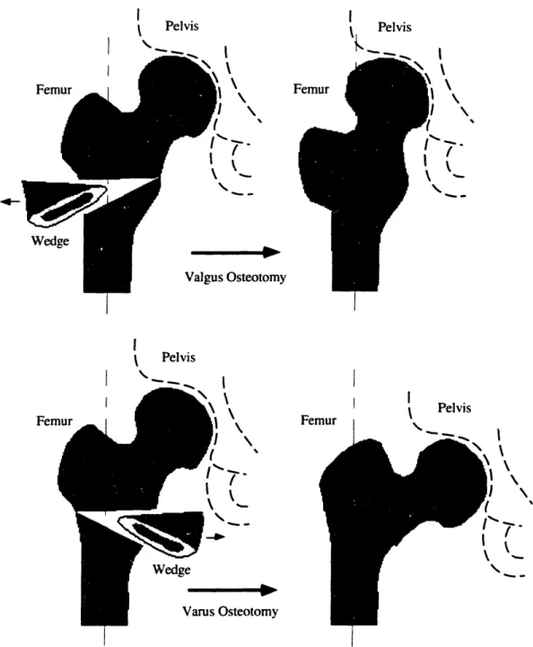
Intertrochanteric osteotomies most commonly fall into two distinct classes, Valgus and

Varus, depending on the lateral direction of the reorientation achieved by the procedure.

Figure 1.2 illustrates these two classes of osteotomies. In addition corrections are also performed with intertrochanteric osteotomies to compensate for reorientations in flexion-extension as well as internal-external rotation. Other osteotomies techniques approach the reorientation by performing a single cut along the bone shaft and rotating the proximal segment with respect to the distal one [107]. These methods have been particularly appropriate for the correction of long bone deformities.

--I Pelvis Pelvis Femur I( I I

_I

Figure 1.2: Valgus versus Varus Intertrochanteric Osteotomies

The most common osteotomy surgery planning technique is based on the acquisition of preoperative planar X-ray films and the extensive use of tracing paper. Figure 1.3 depicts the essence of the planning method. In (A), tracing paper is overlaid on top of the X-ray film to capture the outline of the femoral bone. The osteotomy site is chosen at the level shown (in between the trochanters) for two reasons: the site must be in a region of maximum cancellous bone and a strong medial buttress must be left on the distal fragment to insure proper and optimal healing. The tracing is cut along this line and the two pieces are rotated laterally

Patrick J. Lord. Ph.D. . I X I I I I \

until they overlap at the chosen angle (B). The overlapping wedge is then cut away, leaving the femoral tracing corrected (C). If appropriate, a similar procedure can then be performed in the sagittal plane to compensate for flexion - extension and anteversion - retroversion reorientations [128]. Finally the overall osteotomic biplanar wedge can be inferred from the two correction wedges calculated.

A B C

Figure 1.3: Traditional Intertrochanteric Osteotomy Planning

One can readily see that this preoperative technique relies heavily on the knowledge of the three dimensional nature and quality of the cartilage at the joint and the computation of the appropriate reorientation that minimizes "poor" cartilage overlap. Neither are available from the two dimensional X-ray films which explains the difficulties encountered by orthopedists during the surgery planning phase as well as the poor success rates of such procedures. Although many positive results had been obtained through a better understanding of the mechanisms by which osteotomies work [10, 36, 37, 66, 72, 93, 97, 123], this procedure has gone out of favor and been replaced by the THR. However, since osteotomies work well in selected cases [12, 95, 108], since healing of the diseased articular surfaces has been demonstrated in selected cases [7, 22, 95], and since the limitations of THRs have become apparent, it seems reasonable to re-evaluate the role of osteotomies in the treatment of younger persons with osteoarthritis of the hip [81].

The availability of high speed digital computers now allows us to implement models to simulate and better understand the dynamics involved through the repositioning of the femoral head. With the help of such computer modeling, many research efforts [30, 34, 59, 85, 90] have lead to a better understanding of the mechanical changes associated with surgical procedures which alter the relationships of muscles relative to joints. However, at

Massachusetts Institute of Technology

l-I I

the present time, these models have shown their predictive limitations. Most often based on the osteotomic redistribution of forces at the articular surface advocated by Pauwels [95], these models fail to capture the ability of muscles to adapt to their new length over time. Therefore. the assumption that an osteotomy will not alter the ability of muscles to generate forces is arguable. In addition, other investigations [15] also suggest that proximal femoral osteotomies do not have much effect on the forces on the articular surface and conclude that a change in load at the hip is unlikely to be one of the reasons for the beneficial effects when the results of the operations are good. This comes in direct contrast with Pauwels' work which states that a varus osteotomy of 30 degrees reduces the resultant hip contact force by

25% by increasing the abductor muscle moment arm and that a valgus osteotomy of 30

degrees increases the resultant hip contact force by 25% by reducing the abductor muscle moment arm.

Intertrochanteric osteotomies have a number of mechanical and biological effects on the hip joint which make the determination of whether an osteotomy succeeds almost impossible and therefore preclude a clear indication for the procedure in a specific patient case. By focusing our modeling on the cause and the reason of the hip joint problem, the pain resulting from the interarticular cartilage damage, we believe we can obtain a better predictor of surgery recommendation and outcome. Armed with the assumption that the osteotomy planning should be based on compensating for the "poor" cartilage quality overlap, the approach in this investigation concentrates on identifying the three dimensional hip joint geometry and cartilage quality and implementing the analytical and computational tools necessary to calculate the optimal osteotomic wedge.

1.4 APPROACH

Computerized Tomography (CT) and Magnetic Resonance Imaging (MRI) have become popular and common processes in hospital settings. These techniques offer the in v'il'o measurement of the anatomical geometry by permitting cross sectional scans of the pathological joint. The approach taken in implementing the surgery simulation virtual environment database will require a series of scans. allowing inputs from either imaging system to describe patient specific joint anatomy. With experimental data collected with the finest resolutions of CT or MRI both in cadaver and in ivo studies, a method has been devised to extract the quantitative data necessary to characterize the pathology of the joint. Three dimensional models can then be reconstructed [71] from the serial scans to present qualitative displays of the bone structure and thus an important visual aid in comprehending

not only the geometric but also the kinematic relationships in the joint. To this effect, surface skin kinematic data, is collected with a Selspot optoelectronic camera system and processed with the MIT Newman Laboratory TRACK software [4, 61, 73, 74, 79, 88, 89]. Next, automatic evaluation of femoral and acetabular cartilage thickness is performed. Joint congruency and cartilage maps with areas of damage are then assessed to evaluate the feasibility and potential success outcome of an intertrochanteric osteotomy. For example, recommendations are provided to clinicians as to whether an osteotomy is a potentially good alternative to a THR in the specific patient case under consideration. Finally predictive geometric and kinematic optimization algorithms have been implemented to quantify results and ascertain an optimal osteotomic wedge.

1.5 THESIS OVERVIEW

This section contains a brief summary of the remaining chapters. The chapters describe separate investigations which highlight the necessary steps that have been combined to create our computer aided intertrochanteric osteotomy planning system. Each chapter has been written to present the approach and material of a specific issue or method and includes its own introduction, analysis, simulations, results and conclusions.

Chapter 2 pertains to the anatomical data acquisition and the three dimensional reconstruction of the patient specific skeletal information. Two different scanning imaging techniques are presented along with their respective advantages and the protocols adopted. The techniques

implemented for processing the biological images and extracting the pertinent information about the hip joint are then described. Finally, in-vivo and cadaver experimental results are shown and computer algorithms and techniques used to visualize and handle the reconstructed information are depicted. Chapter 3 concentrates on the development of a systematic anatomical coordinate system selection. A method was implemented to define a coordinate system for the anatomical data that is independent of the coordinate system of the data acquisition machine used. This allows us to consistently compare anatomical data sets collected with different systems as well as at different time intervals. This technique also offers a systematic approach to compute the realignment of data necessary to compensate for misorientations in the scanner systems used.

Chapters 4 investigates techniques to evaluate hip joint kinematic congruency and cartilage estimation. The congruency of the hip joint needs to be assessed prior to any osteotomy procedure recommendation. This analysis is achieved through the fitting of optimal known

geometries to the anatomical information. Then, using optimization methods, the cartilage thickness both on the femoral head and inside the acetabulum is estimated. Since this information is not readily available from the scanned information, it was necessary to develop a procedure that allows areas of damaged cartilage to be clearly identified and the joint kinematic center calculated. The algorithms implemented are verified with simulated data and the results presented. Issues of three dimensional cartilage data visualization are also addressed. Chapter 5 pertains to the reorientation of the femoral head inside the acetabulum to maximize the "good" joint cartilage overlap. The optimization algorithm used to compute this angular correction is presented along with test results from simulations. These results are then translated to define optimal osteotomic wedges through an interactive approach that incorporates clinician expertise if so desired. Finally, the approach used to provide clinicians with a qualitative assessment of the potential osteotomy is described. Overall conclusions are presented in Chapter 6 and summarize the results obtained from Chapters 2 to 5. The integration of each part into a complete computer-aided surgery planning system is discussed. The significant contributions of this research work are identified along with the specific issues described in section 1.1 that have been addressed. Finally, future research directions and recommendations are provided at the end of this chapter.

TWO

ANATOMICAL MODELING

2.1 PATIENT SPECIFIC ANATOMICAL MODELING

In connection with surgical reconstructions and simulations, the skeletal surfaces of human anatomy have no known equation permitting their direct duplication and use by computer methods. It is necessary to measure anatomical features at a discrete number of points and to develop methods to build analytical representations of the data. In addition the difficulty in applying a uniform scaling process to a single data set to fit the description of any patient (we all have legs of different length, shapes and aspect ratios), forces the acquisition of patient specific anatomical information and its transformation into a usable three-dimensional database.

Biological structures are very different from a typical engineering object, which often has smooth analytical surfaces and constant material properties. For bone, the geometry problem is more general than simply describing the surface of an unusually shaped object. A cross-section of bone is not uniform, but has large variations in material density and strength. In addition, the non homogeneous distribution of material density within that object can also be of concern. Fortunately, research and clinical practice has begun to make use of remote sensing modalities such as computerized tomography (CT) and magnetic resonance imaging (MRI) which can provide this information.

The medical need to see inside the human body from the outside has been met for many decades by recording the differential absorption of X-rays. A major deficiency of the standard method of radiography is its inability to discriminate among overlapping structures. This deficiency was remedied by the development of X-ray computerized tomography. CT records X-ray data from many different directions and reconstructs mathematically the information to yield cross-sectional views of any part of the body. Although CT scanning is an extremely useful diagnostic tool, its use of X-rays, even in small doses, carries a risk of doing physiological harm to sensitive organs (i.e.: reproductive system). More recently MRI, a new technique for obtaining cross-sectional pictures through the human body without exposing the patient to ionizing radiation has gained popularity not only because it provides information comparable to CT but also because it discriminates more sensitively between healthy and diseased tissue. Both imaging techniques are readily available within the clinical setting and are the basis today of much medical diagnoses through the two-dimensional images they provide of a patient specific cross section.

Since it is important for the reader to have a general understanding of the basic concepts behind imaging techniques such as CT and MRI, brief overviews are presented in the following sections.

2.1.1 COMPUTERIZED TOMOGRAPHY

Wilhem Konrad Rontgen discovered X-rays in 1895, and his imaging technique has been used since then to image tissues areas with large density differences. For example, a shadow projection of a bone can be clearly distinguished from its surrounding soft tissue structures which do exhibit density differences sufficient enough to allow for distinct identification. Moreover, and as noted above, superimposed areas produce an image that is the result from multiple shadows. In 1963, A. M. Cormack conceived the idea of X-ray transmission along lines parallel to a large number of different directions to produce a sequence of X-ray transmission profile and proposed its use in the field of medical imaging [26]. However, it is

only in 1976 that his work was adapted by Robert S. Ledley to an Automatic Computerized

Transverse Axial scanner [70]. ACTA was the first CT scanner with the capacity to produce clear and detailed cross sectional images over the entire human body and was immediately adopted to complement and help physicians with their analyses and diagnoses.

CT scanning can be achieved in different ways. The most common involves both translation along the longitudinal axis of the body and rotation around the cross section of the body that is being examined. For each image at a specific translation coordinate, the mechanical

scanner rotates 180° in 1° or 2 increments to allow for highly collimated X-ray beams to pass through the body section at each position. The next image is generated similarly by acquiring data at a new translational location. While some of the X-rays are absorbed by the body, others pass through and are detected by a scintillation crystal. The intensity of the beam is measured and recorded to create an intensity profile. The absorption pattern projection depends on the sum of the absorption coefficients of the tissues through which the beam passes. By combining many such absorption patterns along the 180° rotation of the scanner the computer can then reconstruct the contribution of sub volume areas inside the cross section being studied. Then, by assigning a value from a gray scale gradient to the intensity of absorbed X-ray transmission by a part of the body, an image can be created which visually identifies the structures within the cross section. Subtle variations in density such as in muscles, ligaments, fat and derm layers are difficult to discriminate while bone provides a high density contrast which can be clearly visualized. It is important to also note that for the particular concern of this investigation, CT does not allow for clear imaging or the cartilage surfaces which because of their particular nature are not easily distinguishable

from the surrounding soft tissue.

While it has been argued that conventional X-rays expose a patient to higher dose of radiation than CT scans do, the use of numerous thin, contiguous CT scans needed to produce three-dimensional anatomical reconstructions raises concerns regarding its invasiveness to patient health. However, it is true that the high collimation of the X-ray beam does not result in much scatter and only exposes a specific and localized area of the body. In addition the cross sectional slices are usually taken far apart to prevent the cumulative radiation exposure. Nonetheless, in cases of younger patients and in areas of high concentration of sensitive organs it is preferable to minimize, if not suppress, the potentially harmful effects of this imaging technique.

2.1.2 MAGNETIC RESONANCE IMAGING

The experimental foundations of nuclear magnetic resonance (NMR) were first discovered by Felix Bloch [9] and Edward Purcell [101] in 1946 and resulted in a Nobel prize award in 1952. While traditionally used in physics and chemistry to investigate molecular composition or monitor metabolic reactions, it is not until recently that NMR was introduced to the medical imaging field and renamed magnetic resonance imaging (MRI). The potential offered by MRI to distinguish between benign and malignant tissue was discovered in 1971

by Damadian and represents the initial application of NMR to a medical field [27]. Lauterbur

then develop an improved MRI technique which used magnetic field gradients and

tomographic reconstruction techniques to produce images [69]. His work was the basis for the implementation of modern MRI systems which yielded the first cross sectional images of

human anatomy in 1977.

Since MRI uses magnetic fields as the source for its imaging method, it does not expose patients to any ionizing radiation and is often considered a very safe alternative to CT. This assumption is commonly accepted in clinical settings and studies have demonstrated that the health risks associated with MRI are minimal [14, 19, 20, 126]. The sources of potentially harmful health effect have been identified and limited to three: static magnetic fields which are less than 2 Tesla (20,000 gauss), changing magnetic fields of 5 mT (50 gauss) amplitude and less than 100 Hz frequency, and radio frequency heating up to 4 W/kg. For most MRI investigations, the exposure to these effects have been found to be well below the known thresholds for health effects. However, while both MRI and CT produce cross sectional images of human anatomy, there are some fundamental differences between the two imaging techniques. Primarily, the signal measured in MRI is related to the density and relaxation

times of the atoms being exited and not to the mass density of the tissue as in CT. The most

common magnetic resonance imaging is based on proton nuclear magnetic resonance and involves the study of the density of hydrogen atoms in the water molecule because of their intrinsic NMR sensitivity and high concentrations in biological material. As a result, MRI measures several parameters that, once combined, define the intensity of the image pixel at the particular location of the molecule being examined. These parameters are the longitudinal or spin-lattice relaxation time, the transverse or spin-spin relaxation time, and the density of the magnetic nuclei [13, 32]. By combining these parameters with different and suitable weighting techniques, it is possible to create an image that provides the contrast necessary to highlight specific tissue areas proportionately to the molecular environment being imaged.

The principles behind MRI imaging rely on the use of a static magnetic field to align atoms with naturally occurring magnetic dipoles together with a short pulse of a radio frequency (RF) magnetic field that perturbs the atoms [102]. The maximum signal can be observed immediately after the initialization of the RF field where the magnetic moments of the excited nuclei are all lined up in their new orientation along the direction of the superimposed RF magnetic field. This signal then decays over time in two ways. The first one corresponds to a slow down of the spin system until thermal equilibrium is reached within the lattice structure and is known as the spin-lattice relaxation. The second one represents the dephasing or misalignment of the nuclear magnetic moments which create a local magnetic field and is referred to as the exponential decay of the spin-spin relaxation. The sum of the

static magnetic field and the surrounding fluctuating fields determines the total field at a nucleus. Finally, the greater the number of magnetic nuclei present, the larger the NMR signal. This density parameter determines the contrast of the NMR image.

The fact that MRI images can be most easily generated from the resonance of hydrogen nuclei is fortunate because the human body is 70% water. It also indicates that MRI has the ability to image soft tissues and distinguish among different ones such as muscles, tendons, ligaments and cartilage with a higher contrast than CT can and explains why most MRI scans are now used for brain and spinal cord studies to assess the existence and location of tumors. MRI is therefore well suited to the visualization and determination of body segment mass and inertial properties [17]. It should be noted though that since bone material holds little water content, and thus fewer hydrogen atoms, its imaging via MRI does not have the accuracy that is offered by CT. However, and most importantly, MRI does not expose subjects to harmful radiation and therefore lessens the potential health risks when compared to computerized tomography.

2.1.3 DATA ACQUISITION PROTOCOL

Since both CT and MRI are readily available in clinical settings, this investigation implemented an approach to three-dimensional anatomical modeling of the hip joint that is independent from the data acquisition method chosen. Since each imaging modalities has unique advantages and limitations, this approach allows clinicians to choose the most appropriate imaging technique depending on a compromise between the patient's age, health risks and benefits, and the accuracy sought for the three-dimensional reconstruction. However, it is the belief of this investigation that MRI should be the preferred in-vivo method over CT because of the necessity to acquire multiple thin slices in an area of the human anatomy that would be most sensitive to X-ray over-exposure. Even though today CT provides higher resolution and more accurate images of skeletal information than MRI, future developments in MRI technologies related to extensive testing for its applications throughout the body will overcome present drawbacks. A discussion of the protocol used for CT on cadaver material and for MR imaging in in-vivo experiments follows.

A protocol was designed to acquire data with the highest possible resolution and density. Standard GE transaxial CT and MRI scans were obtained on a cadaver leg and subjects respectively. The resolution achieved with CT was 310 gim with a 512 x 512 pixel image. The MRI resolution was 930 gm and resulted in a 256 x 256 image. The scanners were recalibrated prior to any experiment with the phantoms provided by the manufacturers. The

body areas under interest were positioned in the center of the scanner field to minimize the effects of nonlinearities particularly evident at the edges of the viewing field. Figure 2. 1, the scout view from a CT scan on a cadaver leg, illustrates the "slicing" protocol adopted. Slices with the thinnest thickness (1 mm for CT and 2 mm for MRI) were taken at the hip joint with the shortest distance apart (1.5 mm for CT and 3 mm for MRI) whih still preventing signal coupling among slices during image reconstruction. For MRI, the pulses associated with the relaxation times T 1 and T2 were chosen to maximize the imaging of bone structures. Finally. slices set further apart were obtained only for qualitative three-dimensional modeling along

the distal area of the femur and in the upper part of the iliac crest. More specifically, the data

acquisition protocol specifies for 5 mm contiguous slices from the crest of the ilium to a point just superior to the acetabulum, 1.5 mm contiguous slices (3 mm for MRI) through the

femoral head until the inferior part of the lesser trochanter, and then 10 mm contiguous slices down the femoral shaft to a point at least 15 cm distal to the lesser trochanter. In the area of highest slice density, an exposure to around 2.5 rads can be expected with CT scanning.

While using image enhancers has become very common to highlight specific anatomical features during medical imaging, its invasiveness in the case of hip joint imaging makes it impractical as a standard approach. Radio and magneto opaque dyes, such as gadolinium, monosodium urate, or calcium pyrophosphate, would have to be injected in the joint capsule to promote the detection of the inter-articular gap by the imaging technique considered. Studies [8] have shown that such procedures not only present health risks for patients but also do not guarantee better visualization of the joint space. This is in part due to the poor infiltration of the dye inside the joint capsule, and its poor diffusion through the synovial fluid. Therefore, this research project opted to collect anatomical information without requiring the use of image enhancing dyes. This makes for much simpler and safer clinical protocols that limits themselves to the health hazards associated with medical scanning systems. At most hospital medical imaging centers, a data acquisition session can be completed in about one hour and at cost of about $900 for CT and $1300 for MRI. The scanner output can be displayed on the system console where it can be manipulated to adjust for brightness and contrast. The resulting image can then be presented on film, similar to X-ray radiographs, as well as stored digitally on magnetic media for further processing. Appendix A presents the different data sets collected for this study with CT and MRI both on cadaver material and patients.

FiLure 2. 1: Scanner Slicing Protocol (Cadaver CT Scout View )

Standard experiments result in more than 200 irmages ith a storae capacit need of' o\ er

t1{() Nlteall\te . The lrmaI, ga(thered were stored on magnetic tape, and transfcrred to the o\\,rkstation ,\ ,tem hard disk ued for the image manipulation and computer-alded urgerx ,, ,,to1m i1mplemientation. Proprictar header information was ,tripped from the image file., x, hich x cre then tored as binary data matrices in either l '2 x 5 1 2 or 256 x 256 Lrid,.

2.1.4 COMPUTING AND DISPLAY ENVIRONIMENT

A Silicon Ciraphics Personal IRIS 4D35TG workstation was ued to tore the raw and

converted scan data and enerate the 2-D contour data and the 3-D surface mesh

reconstructioon. The computer. based on a 33 NIHz MIPS R4000 RISC microprocessor. provides an integer performance of 35 million instructions per second (MIPS and b million

l'loating pint operation, per second (ltlops). In addition this computer svtncJ11 offers for

display purposes a graphics raster subsystem based on a high-performance, high-resolution color three-dimensional geometry pipeline engine to handle display transformations

(translations, rotations, scaling, and viewing transforms of points, vectors and polygons), matrix manipulations, lighting, material properties, shading, color and texture mapping. The computer operated under IRIXTM_{, a UNIX}T M _{operating system compliant with the AT&T} System V Release 4 standard. While a confounding variety of graphics computer hardware commercially available today and supported by different software would have most likely produced the same results and accomplished the same goals, the balance of real-time simulation, computation power, three-dimensional graphics technology, and interactive device /10 offered by SGI workstations was found invaluable for this research project. In

addition, the recent standardization of OpenGLTM_{, the three-dimensional graphics}

programming library pioneered by SGI, among multiple hardware vendors makes the implementation of this computer-aided surgery system cross compatible with other workstations (HP, Sun, IBM, ... ).

I

_____*____

Monitor

Figure 2.2: Silicon Graphics Computer System Environment

The programming language adopted for the software implementation was C [63]. This decision was due largely because of four major lines. First, the block structure provided by C allows developers to divide large programs into smaller files and functions and to create their own flexible data structures. Second, C is a pointer, or address, based language that, as opposed to value oriented languages, permits the fast and efficient manipulation of large data structures not uncommon to biological databases. In addition, this feature permits the dynamic memory allocation necessary to handle data sets of unknown and variable sizes and optimizes the sharing of computer system memory resources. Third, by logically connecting input devices (mouse, tablet, trackball, ...) to the display transformations, C simplifies the development of code that allows the user to interact in real-time with the on screen

.s..scclWhu.setts Institute of Technolo gy' Operating system File Mangement Applications Software Development ~r rrsr tcI ,Lornrw 1/0 Disk Storage Memory Network Keyboard Mouse Geometry Pipeline Frame Buffer Controller

Z-buffers Lighting Models Shading Color Maps - - ---- I1-

information. Finally. the versatility and recent popularity of C made it the programming language of choice to plan for further future development of the project. Most of the software developed as part of this research is presented in the appendices: the following sections and

chapters will direct the reader to the appropriate appendix to use as a reference.

2.2 SEGMENTING

CT and MR imaging provide clinicians with two-dimensional cross-sectional images of the human anatomy that contain vast amounts on information. There is a need to reconstruct this information in three dimensions, but also to extract the information needed out of the images selected. For example, if interested in the skeletal data. one should be capable of discarding the soft tissue information and vice-versa. To this effect, a program to generate viewable anatomical structures from multiple serial CT or MRI scans has been developed as part of this project. While other studies have developed similar techniques. our goal was to identify the soft tissues and bones. isolate the bones, and segment them into individual databases with as little human intervention as possible. If the concept of computer aided surgical systems is to be successful in the clinical setting, anatomical reconstruction software will have to be used by paramedical personnel and accomplished as quickly and as effortlessly as possible. First. we focus on the extraction of skeletal features from scanner images.

2.2.1 THRESHOLDING

For each image slice, the bone structure was isolated and extracted from the rest of the anatomical information. In the case of CT. each image pixel represents a Hounsfield CT number. Thus, to separate bone tissue from the other tissue densities, a single Hounsfield number. or a range of CT numbers was chosen. Even though MRI contrasts human anatomy differently, the methods used to process these images were inherently the same with some adjustments to the MRI parameters chosen. The main difference results from the fact that some soft tissue structures in MRI images can have pixel intensity levels very close to bone and sometimes even higher. Bone material can then be comprised in a very narrow band of intensities which makes it necessary to eliminate information that can be not only darker but also brighter than bone. However, this process can be done rapidly with some trial and error. Figure 2.3 shows a three-dimensional representation of a femur cross-section image before (a) and after thresholding (b). Finally, the image is transformed with a binary filter to identify bone in white and the rest of the information in the image in black (c).

I/vcr~~~~~~~~/

150 l

1001

50

C

(a) Raw Medical Ima;e

150 100

5(

(b) Image Thresholded to Delete Soft Tissiue Information.

200'

100 0

(c) Binary Image : bone is in white. an\ything else in black. Figure 2.3: Thresholding Process

0 I I I I I 1 f F I I! " ,,, ,1.11 (:: fill W 'T,, hii,

One will note that, as expected, the CT image presented in figure 2.3 does not discriminate well among soft tissues (the waves that can be observed in the image background are signals corresponding to the presence of the plastic bag used to contain the cadaver specimen). Bone tissues stand out and can easily be identify and extracted by choosing an appropriate CT number. This will vary between experiments, but a Hounsfield unit of 176 was found to be a good thresholding number for bone tissue. The thresholding value in the case of MR images greatly varies with the parameters chosen for the magnetic relaxation times and the radio frequency decay of a particular scan set. Therefore, for each MRI experiment, the images were analyzed to derive the best thresholds.

Several studies have investigated the accuracy and precision of CT and MRI systems. For CT, numerous factors, including beam hardening, partial volume effects. medullary fat content and image display parameters can affect quantitative analyses of the reconstructed images. While thickness measurements of soft tissues can result in errors as high as 30%. Sumner et al. [112, 113] found that periosteal bone diameters were accurate to +1.0% with endosteal diameters only accurate to ±4.6% because of the consistent over-estimation of the medullary dimensions. In addition, Woolson et al. [127] confirmed these findings by showing that external linear dimensions (perimeters) of CT based femoral shaft models were within 3 mm (+1.5%) of actual measurements while medullary canal models were consistently smaller than the actual specimen. Finally, Smith et al. [111] demonstrated accuracies of 99.0% for CT and 97.5% for MRI based reconstruction of femoral bones by comparing Bridgeport milled slices from image data with caliper measurements directly over the carefully positioned specimen with and without the overlying soft tissues.

Table 2.1: CT and MRI Accuracy Sensitivity

CT MRI

Elasticity Variation Elasticity Variation

Perimeter 0.019 +0.95% 0.035 +1.76%

Area 0.116 +5.82% 0.179 +8.93%

In this study, we investigated the elasticity or the ratio of percentage change of bone area and perimeter variations over the percentage change in image threshold value since we were interested in the external dimensions of the reconstructed information. Our results, presented in table 2.1, confirm previous study findings. Elasticities were found to be small suggesting that only large changes in threshold values result in small changes in bone perimeters and areas. As expected, results are better for CT than for MRI and area measurements are more sensitive than perimeter dimensions to threshold variations, this being mostly due to larger

errors in bone marrow evaluation. All calculations were performed in pixel base units. Three-dimensional reconstructions of femur anatomy based on CT or MRI are spatially accurate and unaffected by the presence or absence of soft tissues. Oblique slices can accurately and reproducibly be used to reconstruct and characterize articular geometry. CT provides better assessment of calcification, ossification, and periosteal reaction while MRI represents the most accurate imaging modality for evaluating intramedullary and soft tissue extent. In addition, although CT offers better resolution and accuracy, MRI remains the imaging modality of choice for obtaining in-vivo patient specific joint anatomy information due to the reduced health hazards.

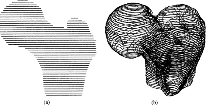
2.2.2 CONTOURING: EDGE DETECTING

To further the reduction in the amount of information to be manipulated by the computer, the thresholded images were contoured to extract the edges of bone information. The three-dimensional tile representation provided by stacking all two-three-dimensional thresholded images provides a clue to the three-dimensional nature of the data and has been extensively used by many investigators [6, 33]. However, the amount of data does not permit real-time manipulation of the anatomical information even with specialized three-dimensional graphic hardware. The adoption of contour representation allows the operator to reduce the information to the essential of the investigation. Other studies [129, 130] have adopted this technique which is often referred to as the ring-stack representation. These one dimensional unit based approaches consist of delineating the surfaces of an object which intersect with a set of slice. This results in a stack of borders that represent the surfaces of the object and the object itself. As in all feature extraction problems the main theme is which are the best cues for extracting the features. This depends on the definition of the feature to be extracted; by previously thresholding the images, the nature of the feature to be extracted involves directly large intensity variations between a region and another one. The obvious cue will be the intensity difference, or a weighted difference of intensities within a specified neighborhood. This approach has indeed been followed for many years by a wide number of authors in the feature extraction imaging field [109].

The edge detection algorithm implemented in this study is mostly based on the first and most intuitive approach which is to extract the pixels belonging to an edge, thus using a gradient

transformation on the digital image so as to detect local intensity variations [57]. In addition,

gradient based methods, while very sensitive to noise in the image, provide a very good criteria for edge detection in the case of a thresholded binary image, where the background

has been normalized to zero. For continuous two-dimensional functions, the gradient is given by:

Vf(x,y)

(i

+

.J

(Eq. 2.1)

with its magnitude defined as:

IVf(x,y)I=

)

and the orientation of the gradient vector:

dcfJ

a = Tan' -, (Eq. 2.3)

But when operating on a discrete, or digital, image, x,y and f(x,y) are non negative integer numbers so that the partial derivatives must be approximated with finite difference along the two orthogonal directions x and y, thus resulting in:

Vf(x,y) = f(x,y) - f(x - l,y)

(Eq. 2.4)

Vf(x,y)

where x and y are pixel positions and f(x,y) is the pixel intensity value. Then, for any orientation ca we have:

Vf(x,y) = f(x,y)cos(a) + f(x,y)sin(ca) (Eq. 2.6)

Thus the digital approximation to the magnitude of the gradient of f(x,y) can be given as

IVf(x,y)l = ,Vxf(Xx,y)2+ Vf(x,y) 2 (Eq. 2.7)

To simplify this expression, and speed up computation, it generally happens that the digital gradient magnitude is approximated to be either the sum of the absolute' values of the two-directional increments or the maximum between these same two increments:

jVf(x, )j =lVf(x,y)I + IVf(x, y) (Eq. 2.8)

or

JVf(x. y)J - MAX(Vf(x, Y)I, IV f(x, y)I) (Eq. 2.9)

These approximation are dependent on orientation as investigated by Deutsch and Fram [31]. The process then involves the evaluation of the digital gradient at the eight pixel neighbors

using:

fl.,(X, y) = MAX(f(x. y) - f(l,m)) (Eq. 2.10)

where I and m are the coordinates of the eight neighbors of the pixel located at x, y and

depicted in Figure 2.4.

II

e~

I

Image Pixel and Neighbor Coordinates on an m x n Digital Image

Figure 2.4: Definition of Image Pixel and Neighbors

The orientation of the gradient a corresponds to the gradient magnitude that is found to be the maximum. Then, the process continues by following in this direction the path, pixel by pixel, until a loop is closed thus resulting in a contour. One will notice that the identification of the initial pixel can be critical in the contour extraction process. Several studies have tried to fully automate this process [116], however, this project opted for operator intervention to select the initial point and thus optimize performance. This user action permits not only the selection of internal startup pixels to produce contours of the endosteal area of the femoral shaft but also the identification of contours of different bone structures in the joint area (i.e.: contours defining the femoral head as opposed to the ones defining the pelvis acetabulum.) thus providing bone segmentation with relative ease. In addition, this manual selection, performed by operators directly on the screen with mouse control, limits the evaluation of contours to the surfaces of interest and does not result in the production of a multitude of

A1a.s.achusetts Institute of Technology

X-I

-contours. a definite drawback of fully automatic contouring algorithms in the presence of complex anatomical shapes.

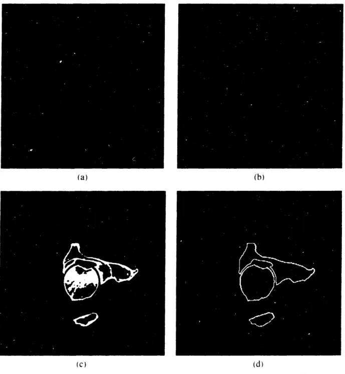
2.2.3 RESULTS

(a) (b)

(c) (d)

Figure 2.5: Image Processing from Raw Image (a) to Segmented Contour (d)

The contouring algorithm is an integral part of the overall program used for image viewing

and thresholding. For reference purposes. this software is presented in its entirety in

Appendix B. The process of segmenting a complete data set can be performed bx an operator