Computational study of rotating stall in high-speed compressor

Computational Study of Rotating Stall in High-Speed

Compressor

by

Jun Luo

B.E. Aerospace Engine, Beijing University of Aeronautics and Astronautics

Beijing (1998)

Submitted to the Department of Aeronautics and Astronautics in partial fulfillment of the requirements for the degree of

MASTER OF SCIENCE IN AERONAUTICS AND ASTRONAUTICS at the

MASSACHUSETTS INSTITUTE OF TECHNOLOGY

May 2003

© Massachusetts Institute of Technology 2003. All rights reserved.

MASSACHUSETTS INSTITUTE

OF TECHNOLOGY

SEP 1

0

2003

LIBRARIES

A uthor ...

Department of Aeronautics and Astronautics MayZ3, 2003

Certified by ...

Yifang Gong, Thesis Advisor Research Engineer

Certified by ...

Choon S. Tan, Thesis Advisor Senior Research Engineer

Accepted by ...

Edward M. Greitzer H. N. Slater Professor of Aeronautics and Astronautics Chair, Committee on Graduate Students

Computational Study of Rotating Stall in High-Speed Compressor

Jun Luo

Submitted to the Department of Aeronautics and Astronautics on May 15, 2003 in partial fulfillment of the

requirements for the degree of Master of Science in Aeronautics and Astronautics

Abstract

A computational study of compressor instability based on body force representation of each blade-row of a transonic stage has been implemented for both clean inlet flow and flow with circumferential total pressure inlet distortion. The computational results indicate that many aspects related to compressor instability differ from what was observed in the experiment: steady compressor characteristics, stalling mass flow as well as the key details in stall inception process. The discrepancy has been attributed to the inadequacy of the body force formulation, which only reproduces the design operating point of the research compressor. In order to overcome this inadequacy, a procedure is proposed and implemented to modify the compressor body force based on the experimental data to match the stalling mass flow and compressor characteristic slope near stall. To assess the adequacy of the modified body force formulation, instability calculations incorporating the modification are carried out for both clean inlet flow and flow with circumferential total pressure inlet distortion. The modified body force formulation gives a computed stalling mass flow in agreement with measured value. While it also yields the modal type stall inception that are in agreement with experiment for clean inlet flow, the computed stall inception with inlet distortion differs from experiments in which the stall inception is through spike followed by modal wave disturbance. The calculations with inlet distortion show that both the compressor performance and the stability margin deteriorate.

Thesis Supervisors: Yifang Gong Research Engineer

Acknowledgements

Many people have given me a lot of help in this thesis and made my life at MIT more enjoyable. I would like to express my deep gratitude to them.

First and foremost, I would like to thank my advisors, Dr. Yifang Gong and Dr. Choon S. Tan for their guidance and support throughout this project. Much gratitude is also extended to Dr. James D. Paduano for his guidance, lots of help and financial support. I would also like to express my sincere thanks to those professors who taught me the courses at MIT: Professor Epstein, Professor Greitzer, Professor Spakovszky, Dr. Tan, Professor Drela in Department of Aeronautics and Astronautics; Professor Sonin and Professor Mckinley in Department of Mechanical Engineering. I believe all the knowledge I have learned at MIT will benefit my future development and even the whole life.

In addition, I am also thankful to the staff and graduate students of Gas Turbine Laboratory. Paul Warren, Julie Finn, Holly Anderson, Dongwon Choi, Brenda Macleod, Beilene Hao, Andrew Luers, Neil Murray, Yong Wang, Yiben Lin, Lixian Liu, Deborah Pilczer, Sebastien Akouche, Jhongwoo Peck, Bobby Sirakov, Van-Man Lei, Chiang Juay Teo, Benny Chi Kin Yam, Dr. Hongwei Sun, Dr. Shengfang Liao. Their friendship and help has been invaluable and is well appreciated.

I would like to thank my family, my parents and my sister for their continued moral support throughout all the time that I have spent at MIT.

Last but not least, I would like to thank my girlfriend Lingling Li for her moral support and encouragement.

This research was funded by the U.S Air Force under a Grant F49620-00-0014 and its support is gratefully acknowledged.

Centents

1. Introduction...1

1.1 Introduction...1

1.2 Overview of Compression System Instabilities...1

1.1.1 Types of Instability in Axial Flow Compressors...2

1.1.2 Onset of Instability...3

1.1.3 Stall Inception...5

1.3 A Review of Current Modeling for Rotating Stall...8

1.1.1 Stall Propagation Mechanism...8

1.1.2 Zero Slope Instability Criterion...9

1.1.3 Moore-Greitzer Theory...10

1.1.4 Three-Dimensionality and Non-Linearity of Rotating Stall...11

1.1.5 Inlet Distortion Effects on Compressor Operability...13

1.4 Research Objectives...17

1.5 C ontributions... 17

1.6 Thesis Organization... 17

2. Computational Flow Model for High-Speed Compressors...19

2.1 Modeling of a Compression System...20

2.1.1 Flow in Ducts... 21

2.1.2 Flow in Blade-Rows...21

2.1.3 Plenum and Throttle...22

2.2 Formulation of Body Force... 23

2.1.1 A Form of Body Force for Representing a Blade Passage...23

2.1.2 Body Force Formulation Proposed in Gong [9]...25

2.3 Numerical Method... 27

2.4 Sum m ary...28

3. Instability Calculation of a High-Speed Compressor... 30

3.1 NASA Stage-35 Compressor ... 30

3.2 Instability Calculations... 33

3.2.1 Clean Inlet Flow... 38

3.2.2 Flow with Circumferential Total Pressure Inlet Distortion... 39

3.3 Comparison of Computational Results with Experimental Data..40

3.4 Sum m ary... 41

4. Body Force Calibration of Stage-35 Compressor and Instability Calculations based on Calibrated Body Force... 52

4.3 Instability Calculations Using the Modified Body Force...53

4.3.1 C lean Inlet Flow ... 53

4.3.2 Flow with Circumferential Total Pressure Inlet Distortion . 55 4.4 Summary... 56

5. Summary, Conclusions and Future Work...64

5.1 Summary... 64

5.2 Concluding Remarks... 64

5.3 Recommendations for Future Work... 65

B ibliography...

66

Appendix I. Post Process of Computational Results...70

I. Spatial Fourier Transform... 70

II. Fourier Collocation Method... 70

Appendix II. Detailed Calibration Procedure of Compressor Body Force.72 I. Determination of the Body Force from a Three-Dimensional Flow in a B lade Passage... 72

II. Deducing

f,

f,

III. Calibration Procedure... 74

Appendix III. Introduction and Solution of Ill-Posed Problem... 91

I. Introduction...91

II. Solution of Ill-Posed Problem ... 91

III. Choice of Regularization Parameter... 92

List of Figures

1.1 Basic components of a compression system...2

1.2 Three types of compressor instability characterized in terms of the respective pressure rise characteristics...3

1.3 Three types of instabilities in a compression system characterized in terms of respective flow field... 3

1.4 Velocity traces of eight sensors around the compressor annulus show a typical modal w ave stall inception process [17]...6

1.5 Velocity traces of eight sensors around the compressor annulus show a typical spike stall inception process [4]... 6

1.6 A model for determining the stall inception type of a compressor [21]... 7

1.7 Physical mechanism for stall inception process [5]... 8

1.8 Static argument showing why negative slopes are stable whilst positive ones are unstable [39]... 10

1.9 Effect of Inlet Distortion on Axial Compressor Performance and Stability [24] .. 14

1.10 Two types of compressor resonance response to rotating inlet distortions [26]...16

2.1 Illustration of a compression system... 20

2.2 Flow in a blade passage is modeled locally as a flow in a straight channel... 24

2.3 Body force due to pressure gradient in a staggered channel... 25

2.4 Illustration of fluxes evaluation around a cell in the blade row region...28

3.1 Rotor and stator of NASA stage-35 compressor... 31

3.2 Computational domain of NASA stage-35 compressor... 32

3.3 Computational mesh in meridional plane...33

3.4 Computational mesh at inlet face... 33

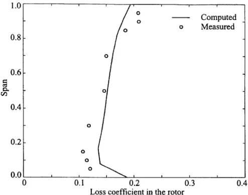
3.5 The computed and measured loss coefficient profile of Rotor 35 at 100% rotational speed and 20.2 kg/sec mass flow rate [9]... 35

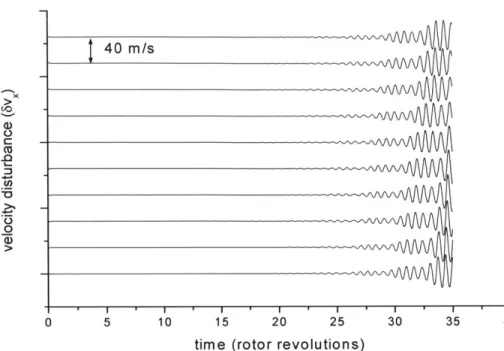
3.6 The computed and measured deviation angle of Rotor 35 at 100% rotational speed and 20.2 kg/sec mass flow rate [9]... 35 3.7 Computed Vx traces in rotor tip exit during stall inception process (spike-shaped

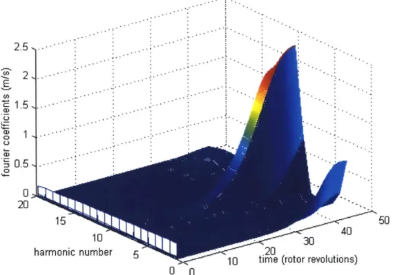
3.8 Evolution of Fourier coefficients of computed Vx in rotor tip exit for the first 15

harm onics... 43

3.9 Harmonic distribution for t=33.18 rotor revolutions... 44

3.10 Computed flow coefficient contour on rotor exit plane(t=3 3.18 rotor revolutions)..44

3.11 Computed Vx traces at rotor tip exit during stall inception process (long wavelength wave disturbance as initial disturbance)...45

3.12 Evolution of Fourier coefficients of calculated Vx at rotor tip exit for the first 15 harm onics... 45

3.13 Harmonic distribution for t=35.32 rotor revolutions... 46

3.14 Flow coefficient contour at rotor exit (t=35.32 rotor revolutions)... 46

3.15 Velocity disturbance traces in rotor tip inlet (flow with inlet distortion)...47

3.16 Comparison of compressor characteristic for clean inlet flow and inlet distorted flow ... . . 47

3.17 Comparison of compressor characteristics by computation and measurement...48

3.18 Experimental data for rotor deviation angle (70% speed)...48

3.19 Experimental data of rotor loss coefficient (70% speed)... 49

3.20 Computational results for rotor deviation angle for different mass flow... 49

3.21 Computational results for rotor loss coefficients for different mass flow...50

3.22 Stall inception process for clean inlet flow in [35]... 50

3.23 Circumferential inlet distortion without blowing: initial spike and then modal pre-stall behavior [46]... 51

4.1 Computed Vx traces on rotor tip inlet during stall inception process (spike-shaped disturbance as initial disturbance)... 57

4.2 Evolution of Fourier coefficients of computed Vx on rotor hub inlet for the first 15 harm onics... 57

4.3 Harmonic distribution for t=42.7 rotor revolutions...58

4.4 Flow coefficient contour at rotor inlet (t=42.7 rotor evolutions)... 58

4.5 Computed Vx traces in rotor tip inlet during stall inception process (modal-shaped disturbance as initial disturbance)... 59

4.6 Evolution of Fourier coefficients of calculated Vx in rotor tip inlet for the first 15 harm onics... 59

4.7 Harmonic distribution for t=1 14.5 rotor evolutions... 60

4.8 Flow coefficient contour at rotor inlet (t= 114.5 rotor revolutions)...60

4.9 Flow coefficient contour on rotor exit shows the final stall pattern is "ring stall"...61

4.10 Rotor deviation angle comparison by measurement and calibration for two operating points near stall...6 1 4.11 Rotor deviation difference for the two operating points near stall...62

4.12 Computed Vx traces on rotor tip inlet for flow with inlet distortion... 62

4.13 Flow coefficient contour on rotor exit shows the final stall pattern is "ring stall"... 63

4.14 Comparison of compressor characteristic for clean inlet flow and inlet distorted flow ... . . 63

A. 1 Rotor deviation distribution along blade span (mass flow=11.8 kg/s) ... 81

A.2 Rotor loss coefficient distribution along blade span (mass flow=l 1.8 kg/s)...81

A.3 Rotor deviation distribution along blade span (mass flow=13.5 kg/s) ... 82

A.4 Rotor loss coefficient distribution along blade span (mass flow= 13.5 kg/s)...82

A.5 Stator deviation distribution along blade span (mass flow=1 1.8 kg/s)... 83

A.6 Stator loss coefficient distribution along blade span (mass flow=1 1.8 kg/s)... 83

A.7 Stator deviation distribution along blade span (mass flow=13.5 kg/s)... 84

A.8 Stator loss coefficient distribution along blade span (mass flow=13.5 kg/s)...84

A.9 Rotor deviation angle by measurement and calibration (mass flow=1 1.8 kg/s)... 85

A.10 Rotor loss coefficient by measurement and calibration (mass flow=1 1.8kg/s)... 85

A. 11 Stator deviation angle by measurement and calibration (mass flow=11.8 kg/s).... 86

A. 12 Stator loss coefficient by measurement and calibration (mass flow=1 1.8 kg/s)... 86

A.13 Rotor deviation angle by measurement and calibration (mass flow=13.5 kg/s)... 87

A. 14 Rotor loss coefficient by measurement and calibration (mass flow=13.5 kg/s)... 87

A. 15 Stator deviation angle by measurement and calibration (mass flow=13.5 kg/s)...88

A.16 Stator loss coefficient by measurement and calibration (mass flow=13.5 kg/s)... 88 A.17 Comparison between measurement and computation for stage total pressure ratio.89 A. 18 Comparison between measurement and computation for rotor total pressure ratio.89

Chapter 1

Introduction

1.1 Introduction

The compressor is one of the three primary components of a gas turbine engine (the other two being the combustor and the turbine). As the mass flow through the compressor is decreased, the angle of attack increases, the pressure rise across the compressor increases, this trend continues until a point is reached where the flow cannot sustain the pressure rise across the compressor and the flow through the compressor becomes unstable. Loss of stability is undesirable, as the amplitudes of the unstable oscillations are often very large and can cause severe damage to the compressor blades. In addition, the loss of stability is accompanied by a significant loss in pressure rise. To avoid such instabilities, the compressor (hence the engine) has to work at an operating point corresponding to lower pressure ratio so that an adequate stall margin is maintained. The stall margin can be considerably reduced in operating environments for which the inlet flow conditions are non-uniform.

1.2 Overview of Compression System Instabilities

Conceptually, a compression system is represented by a series of components comprising 1. Inlet duct, which provides the necessary mass flow for the compression system

2. Compressor, which is the core component of the compression system and produce pressure rise.

3. Plenum, which is used to store the mass flow and acts like a combustion chamber 4. Throttle, which is used to regulate the mass flow through the compression system and acts like a turbine.

Plenum

throttle

Fig. 1.1 Basic components of compression system

1.2.1 Types of Instability in Axial Flow Compressors

Three types of instability behavior have been observed at compressor operating points beyond the instability point. They are progressive stall, 'abrupt' stall, and surge. They are characterized in terms of pressure rise characteristics (Fig. 1.2) and flow field respectively (Fig. 1.3).

With progressive stall, there is a gradual deterioration of pressure rise. The pressure rise characteristic is shown in Fig. 1.2 (a). This happens for example when a multistage compressor is operated at a speed below the design speed. The flow field associated with this type of instability is illustrated in Fig. 1.3 (a) which shows several part-span stall cells rotating around the annulus. This flow pattern usually occurs in one or several stages in a multistage compressor.

Abrupt stall features with a sudden drop of pressure rise at the compressor performance map, with the formation of a full span stall cell (stall cells that extend from hub to tip). The stall cell has an axial extent that encompasses the whole compressor; this explains the large drop of pressure rise (in comparison to the situation in the part-span stall cell pattern). To recover from this type of stall pattern, the throttle has to be moved to a position corresponding to a corrected mass flow much larger than that at which the compressor would stall upon throttle closing. This effect is usually referred to as hysteresis, shown in Fig. 1.2 (b).

oscillations where the entire compression system depressurizes and repressurizes, forming the surge cycle as shown in Fig. 1.2 (c). Sometimes, when surge occurs, the flow oscillations are so severe that the flow through the compressor reverses, a flame can be seen at the intake and exhaust as the combustion moves forward and backward from the combustor.

hysteresis

a) Progressive stall b) 'abrupt' stall c) surge

Figure 1.2 Three types of compressor instability characterized in terms of the respective pressure rise characteristics

low flow rate regions

cI

(a) Part span stall (b) Full span stall

Fig. 1.3 Three types of instabilities in a compression system characterized in terms of respective flow field

1.2.2 Onset of Instability

Predicting the condition at which instability will occur in a compressor requires an understanding of the flow processes leading to the onset of instability. The phenomena described in the previous subsection are the final forms of instability. And it's important

(c) Surge

to distinguish the final form from the onset of instability. The transition from initial disturbance to final stall or surge can be usefully divided into three stages (1) inception; (2) development; and (3) final flow pattern. The inception stage is the period when disturbances start to grow (flow becomes unstable). It defines the operating point and conditions for which instability occurs. In practice, the disturbances will take a finite amount of time (from a few to several hundred rotor revolutions) to grow into final stall or surge, so that the inception stage can be viewed as the early development of the unstable flow.

For some compressors, the inception stage consists of the linear growth (extending up to several hundred rotor revolutions) of disturbances of infinitesimal amplitude, while in others the inception stage only extends over one or two rotor revolutions after its detection. The stall inception stage is the major focus of the instability modeling and prediction.

The development stage, which includes all the processes after the inception stage before the final flow pattern to be reached, is usually of less importance. It is often the case that one final form of instability could be the pre-stage of the other final form in the same compressor. For example, rotating stall might cause surge in some compressors, as noted by Greitzer [1]:

Surge is basically one-dimensional phenomenon, involving on overall, annulus averaged compressor performance curve. For typical volumes, lengths, and throttle characteristics must generally be slightly positive sloped for system instability to occur. We have also seen that the axisymmetric flow through a compressor can be unstable to two (three) dimensional infinitesimal disturbances, and that this local instability marks the inception of rotating stall. However, the onset of this rotating stall is very often associated with a precipitous drop in the overall ("one-dimensional") pressure-rise mass flow curve of compressor performance. In other words, the inception of rotating stall can lead to a situation where the instantaneous compressor operating point is on a steeply positively sloped part of the characteristics, with a consequent violation of the dynamic and /or the static instability criteria.

1.2.3 Stall Inception

The stall inception stage is the period when disturbances start to grow and flow field begins to become unstable. Accurate prediction and description of stall inception process are of considerable engineering value in that it defines the stable operating range of the compressor.

Two major inception types have been experimentally identified: modal waves, and spikes. Modal waves are exponentially growing long wavelength (length scale comparable to the annulus) small amplitude disturbances. The rotating speed of this type of disturbance is in the range between 20% to 50% of rotor speed. Modal wave penetrate the whole compressor in the axial direction, so they can be detected by sensors at any locations at the inlet, exit, or within the compressor. Usually, this type of stall inception occurs at a point near the peak of the characteristics and this type of inception can be well described by linear stability theory. Moore-Greitzer model [2] predicted the pre-stall modal wave before measurements were taken [3].

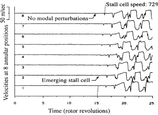
The other inception mechanism is the growth of localized non-linear short wavelength (with length scale of several blade pitches) disturbances [4]. This type of stall inception is referred to as "short wavelength stall inception". The inception starts as one or several spike-shaped finite amplitude disturbances within the tip region of a particular stage. Usually the disturbances develop into a large full span stall cell within three to five rotor revolutions. The initial rotating speed of this type of disturbances is about 70% of rotor speed, substantially higher than that for the typical modal wave speed. Fig. 1.4

shows the velocity traces that lead to rotating stall through modal wave disturbances [17]. From experimental observations, Camp and Day [21] concluded that the spike-type stall inception occurs at a "unique rotor tip incidence". They examined a specific compressor with different IGV stagger angles and found that the stall points line up on a constant rotor tip incidence line whenever the compressor shows spike as its stall inception mechanism. The stall inception mechanism could be switched between modal type and spike-type for the same rotor and stator but with different IGV stagger. The overall trend is that when the first rotor is highly loaded (higher pressure rise for the given flow coefficient), the compressor tends to show spike-type inception, otherwise it shows modal type of stall inception. These experiments suggest that the first-stage rotor

is the key component responsible for the spike-type stall inception. Fig. 1.5 shows velocity traces in the typical spike stall inception process.

53% 3% 50% 46%4 O~ o~Probe #1 Probe #71

I

I

Time (rotor revolutions)

Fig. 1.4 Velocity traces of eight sensors around the compressor annulus show a typical modal wave stall inception process

'Stall cell speed: 72%

5. 10. 15. 20. 25.

Time (rotor revolutions)

Fig. 1.5 Velocity traces of eight sensors around the compressor annulus show a typical C 00 Cz _9_ 4-1 0 C 0 C 0.

Based on their observations, Camp and Day proposed a "unique rotor tip incidence" as a short wavelength stall criterion (Fig. 1.6). When the incidence is reached before the peak of the compressor characteristic, the compressor will stall through short wavelength disturbances; otherwise the compressor will stall at the peak pressure rise and show modal waves as its stall inception type.

Critical Rotor Critical Rotor

Wts Incidence Wts Incidence

peak peak

Modal stall inception Spike stall inception Fig. 1.6 A model for determining the stall inception type of a compressor [21] Based on the above description, some important distinctions between the two kinds of stall inception (modal wave and spike) can be concluded as follows:

1. The number of blade rows that are responsible for their initiation. Spike stall inception is associated with the breakdown of the flow-field in a single blade row. In contrast, the growth of a modal disturbance is associated with an instability of the flow in the whole compressor.

2. The rotating speed of the disturbances in stall inception process. Spike rotates at a faster speed than modal wave disturbances. Usually modal wave disturbances rotate at about 20%-50% rotor speed, while the rotating speed of spike disturbances is about 70%.

3. Mathematical character. Modal wave disturbances are basically linear, their growth are governed by a exponential function of time, while spike disturbance is always associated with separation and three dimensional flow redistribution phenomenon both of which are nonlinear.

1.3 A Review of Current Modeling for Rotating Stall

There are two central issues of rotating stall prediction: rotating speed and instability point, but from the practical point of view, only the instability point is of real concern. Of engineering value is the capability to establish a casual link between instability behavior and compressor design characteristics.

1.3.1 Stall propagation mechanism

The first rotating stall model was the analysis and physical description proposed by Emmons [5]. It can be summarized as follows.

C

B Direction of Stall Propagation A

Compressor blade row Fig. 1.7 Physical mechanism of rotating stall inception

Fig. 1.7 shows that in a row of highly loaded blades, a minor physical irregularity, or flow non-uniformity, can result in momentary overloading and separation. This separation, or blockage, will restrict the flow through the blade passage and will therefore divert the incoming streamlines. When this happens, the flow can separate from the suction surface of the blade so that a substantial flow blockage occurs in the channel between B and C. This blockage causes a diversion of the inlet flow away from blade B and towards C and A to occur (as shown by the arrows), resulting in an increased angle of attack on C and a reduced angle of attack on A. Since C was on the verge of stall before,

tendencies to stall. The stall will thus propagate along the blade row in the direction shown, and under suitable conditions it can grow to a fully developed cell covering half the flow annulus or more. In this fully developed regime, the flow at any local position is quite unsteady; however, the annulus averaged mass flow is steady, with the stall cells serving only to redistribute the flow. Although the sketch only shows one of several possible stall propagation mechanisms, the idea is so intuitive that it is widely accepted by both academic and industrial communities.

Cumpsty and Greitzer [23] used the balance between acceleration in the rotor, stator, and upstream and downstream ducts to argue that the rotating speed of stall cell is determined as the speed at which the unsteady inertial effects in rotors are balanced by the unsteady inertial effects in stationary components. Their model predicted well the measured speed of rotating stall cells. The results also suggest that although the flow redistribution idea is intuitive, the main mechanism for propagation is due to the inertial effects in blade rows and ducts.

1.3.2 Zero Slope Instability Criterion

Perhaps the most well-known instability criterion, which states that the instability will occur at the zero-slope point (peak) of the characteristics, was proposed by Dunham [6]. He found that at zero-slope of total-to-static pressure rise characteristics, the compressor

flow field is neutrally stable, which means the disturbances do not decay.

Gysling examined compressor stability in terms of the net mechanical energy input into the flowfield. A compressor puts energy into a non-axisymmetric flowfield disturbance whenever the total-to-total characteristic has a positive slope (att/a*>O). Mechanical energy can escape since some of it is convected away by the non-steady vortical disturbance in the exit flowfield, and instability will only occur when the compressor puts in more energy than can be convected away (or dissipated in losses). In rough terms, the vortical field carries energy at flow rate "4", the convection speed, and so instability occurs when:

dott/d*~w

or equivalently, since ytt=yts+1/2*2, when

This is the zero slope of the total-to-static pressure rise characteristic condition.

The zero slope stability criterion may be explained by a static style argument based on changes in the local mass flow and pressure rise in Fig. 1.8

Ayts

Unstable

Stable

Local decrease in mass

flow causes increased

pressure rise and results

in locally increased flow

Fig. 1.8 Static argument showing why negative slopes are stable whilst positive ones are unstable

On the negatively sloped pressure rise mass flow characteristics a local increase in mass flow causes a decrease in pressure rise. This causes the flow to decelerate, and the disturbances decay. On a positively sloped characteristic the opposite is true, so any circumferential disturbance is amplified.

1.3.3 Moore-Greitzer Theory

A theory of rotating stall disturbances developed by Moore [7] and a more complete theory of post-stall transients in compressor by Moore and Greitzer [2] are the basis for understanding a different mechanism of rotating stall inception. They assumed that compressor instabilities grow from small amplitude disturbances, and for this reason the linearized form of the equations should accurately describe their initial growth. The inception equations suggest that rotating stall will develop as a result of small flow disturbances that are spatially periodic around the annulus and growing in amplitude. Any spatially periodic disturbance can be represented mathematically as the sum of several pure harmonics (spatial modes) and the growth of any spatial mode can be governed by a exponential function of time.

Although most of the work and development of Moore-Greitzer's model has been for linear cases, the model itself is not limited to small amplitude disturbances. For example, an inlet distortion can be viewed as a stationary large amplitude disturbance. Mathematically, general non-linear disturbances are very hard to be treated analytically; however modem CFD methods can be used to simulate the evolution of any type of disturbances in the system. Longley [17] and Hendricks et al [18] used this idea to simulate instability behavior in high-speed compressors. Escuret and Gamier [19] extended the method to three-dimensional cases.

1.3.4 Three-Dimensionality and Non-Linearity of Rotating Stall

Two-dimensional rotating stall models are limited in that they do not account for flow variations in the spanwise direction. Measurements in compressor rigs indicate that spanwise variations of axial velocity as large as 40% of the mean flow can arise before stall [12]. Reid [24] and Spakovszky et al. [32] showed that radial total pressure distortions at the inlet of the compressor reduced the stalling pressure rise. Gorrell et al. [33] altered casing treatment designs and observed that rotors with the most uniform radial profile of pressure ratio led to the most stable compressors. These results reveal the importance of radial flow variations in affecting the stall point.

Two-dimensional models usually use either a radial average of the flow variation [32,34], or else applied at the mean-radius [35]. To account for the spanwise flow nonuniformity, it has been proposed that the stability of the compressor can be determined by a two-dimensional model at the most unstable spanwise region [36]. The validity of such a proposition is not yet known, although experimental evidence indicates that the location of the stall cell is often linked to the location of highest loading and the lowest velocity. McDougall et al. [36] observed that modal waves had the largest amplitude at either the hub or tip, determined by which region had excessive blockage before stall. Camp and Day [21] found that increased rotor tip loading led to spike stall inception at the outer radius; but increased hub blockage, which diverted the flow outward to unload the tip, led to a modal-type stall inception. On the other hand, Soundranayagam and Elder [37] measured stall inception occurring at the tip of a fan, despite forcibly degrading the root performance; and Jackson [38] detected stall at the tip

of a single stage compressor. All the above work demonstrates the importance of three-dimensionality in stall inception process.

Another important aspect of rotating stall is its non-linearity. Although the linearized analyses have in the past been used to try to predict some of the features of fully developed rotating stall, it has become clear that in this flow regime the stall cells are definitely not small perturbations and linear analysis is not applicable. Thus this type of investigation is only useful for the problem of stall inception, and to follow the subsequent development of rotating stall, one must use a nonlinear model. This has been done by Nakata and Nagano [14], as well as Omer [29]. Extension of these calculation procedures to the case of circumferentially distorted inlet flow has been carried out by Adamczyk [30] and Pandolfi and Colasurdo [31]. These models use time marching techniques to determine whether a small disturbance will grow or decay by calculating the development of the flow to some eventual steady-state solution. This could consist of a flow with a large amplitude disturbance propagating around the compressor, which is taken to be indicative of compressor operation in rotating stall. However, these early efforts [14] did not show much positive results mostly due to the lack of computational resources. Recently, several CFD methods have been used to simulate compressor instability [15, 16]. One advantage of these methods is that they can relate the blade passage events to the instability. One uncertainty of these calculations is that they are performed on a single rotor blade row, since no data are available on short wavelength stall inception in a single rotor. Although CFD can play an important role for implementing computation to provide information on instability behavior that is difficult to measure in a laboratory/test rig, such simulations are still beyond the presently available computational resources for multistage axial compressors.

There is another class of methods that uses both modeling and CFD technique to model the flow in a compression system. These methods could handle three-dimensional nonlinear flow phenomena in a practical manner and require reasonable amount of computational resources. These methods have been demonstrated to be able to compute steady three-dimensional inlet distortion cases [20], long wavelength disturbances in a three-dimensional compressor [19] and disturbances in two-dimensional high-speed

compressors [18]. Conceptually this type of model is able to handle non-linear three-dimensional disturbances (spike) in a compressor.

Gong [9] used body force model, which replace the compressor blades by the body force imposed by the blades to the flow field to simulate rotating stall in GE 4 stage low speed compressor with clean inlet flow. A significant feature of the body force representation is that it is a function of local flow properties. This is essential to model short wavelength disturbances in compressors where flow redistribution occurs in a blade row in the presence of these disturbances. The strength of this computational model is that the compressor is naturally coupled with unsteady three-dimensional flow, so that the model could be used to investigate the interactions between compressor and other components, such as interaction between intake and compressor with inlet distortions, and its impact on the performance and stability margin; The behavior of inlet vortex in an intake and engine, and its impact on the performance and stall margin, etc. Gong also extended the body force model for low speed compressors to high-speed compressors, in which compressor response to inlet distortion was the main focus. However, no effect has been made to quantify the effect of inlet distortion on instability behavior using Gong's formulation, this constitutes the main motivation for the current research focus

1.3.5 Inlet Distortion Effects on Compressor Operability

The above discussions mainly focus on the case with clean inlet flow, which is circumferentially uniform. However, in practice, there are a lot of other factors that can significantly affect the point at which the onset of instability occurs. One of the most important of these is inlet distortion, which is a term used to describe a situation in which substantial total pressure, total temperature, velocity, and/or flow angle variations exist at the compressor inlet face. Aircraft engines are particularly prone to inlet distortion problems due to changes in aircraft altitude and the effect of the airframe on the inlet flow conditions. However, industrial installations can also suffer from inlet distortion in cases where poorly designed bends have been installed upstream of the compressor. In these situations, some portion of the blading is likely to be operating under more unfavorable conditions than would occur with a uniform flow at the same mass flow rate,

An illustration of the effect of inlet distortion on compressor stability and performance is given in Fig. 1.9, which shows data from a nine-stage axial flow compressor [24]. The horizontal axis is the corrected mass flow, and the vertical axis is the total pressure ratio. The dashed lines indicate the measured performance with a uniform inlet, while the solid curves give the measured performance with a circumferential distortion, i. e., circumferentially nonuniform inlet flow. It can be seen that there is a substantial degradation in performance and, more importantly, a large drop in the stability margin due to the inlet distortion. While the consequences may not be this severe with all compressors, there is generally a reduction in the stability of the compression system associated with the presence of an inlet distortion.

7.0

Operating line

Surge line ,'

\

6.0 Surge line with margini

- inlet distortion E 5.0 ''100% W I'l, % 1100% U '97% 4.0 '94% '86% of design 80% rotational speed 3.01 . 25 30 35 40 45 50

Corrected mass flow

Fig. 1.9 Effect of Inlet Distortion on Axial Compressor Performance and Stability [24] Because of the widespread occurrence of inlet distortions, and their adverse effects on system stability, there has been a large amount of work on the problem of predicting compressor response to flow distortion. For example, Mazzawy developed a nonlinear compressible flow model, which can predict compressor performance and stability with a circumferential flow distribution. This model uses multiple parallel compressor segments and accounts for deviations from undistorted compressor performance. Hynes and Greitzer [8] studied the compressor stability with inlet distortion, it is basically an

investigated the effects of rotating inlet distortions on compressor stability in several compressors, and found that there are two types of compressor response (measured in terms of stall margin vs. rotating speed of the distortion): One shows a single resonance peak corresponding to a large decrement in stall margin when inlet distortion is rotating at around 0.4 rotor speed in the direction of rotor rotation (Fig. 1.10 a); the other shows two resonance peaks at 0.3 rotor speed as well as at 0.75 rotor speed (Fig. 1.10 b ). The compressors which show one resonance peak stall through modal waves while the other exhibit the spike type of stall inception. Thus the respective characteristic response of the compressor corresponds to two types of observed stall inception mechanisms which have different impact on stall margin due to inlet distortions.

Minimum flow range with rotating distortion oExperimental data, 500 rpm o Experimental data, 350 rpm Counter Rotation -- f - Co-rotation

0.0 0.5 1.0

Screen rotating speed, in rotor speed (a) Single resonance peak

0.56 0.52 1-CA 0 U -0 0.48 0.44 0.40 0.36 -1.0

Q5 Design point flow coeffici * Uniform flow stall point 0 Experimental data - Calculation Uniform inlet flow range

I4

T

f

Minimum flow range with rotating distortion

-0O~0~ism

Counter rotation do P- Co-rotation

-0.5 0.0 0.5

Screen rotating speed, in rotor speed

1.0

(b) Two resonance peaks

Fig. 1.10 Two types of compressor resonance response to rotating inlet distortions [26].

0.6

t

I

1.4 Research Objectives

A key objective of this thesis is to assess the adequacy of Gong's computational model [9] for simulating instability behavior in high-speed compressor. As noted in Section 1.3.4, Gong's computational model [9] for high-speed compressor has not been applied to simulating compressor instability inception and development in a representative high-speed compressor stage. In addition, the adequacy of the computational model is to a large extent determined by the level of details in body force representation of the compressor blade row. Specifically, we need to address the issue on the level of details needed: is the body force formulation proposed by Gong [9] able to capture the key aspects of instability inception and development in high-speed compressor?

In addition, other important issues that need to be addressed are:

1. The instability behavior of a high-speed compressor with clean inlet flow versus inlet distorted flow;

2. The effect of inlet distortions of different length scale and time scale on compressor operability;

1.5 Contributions

The contributions of this thesis can be described as follows:

While the work constituted a first attempt on using body force representations of blade rows to simulate instability behavior in a high-speed single stage compressor for both clean inlet flow and inlet distorted flow, the results indicate that a body force representation that match the design point performance is not adequate for instability simulation. Modifying the body force representation to match the stalling mass flow and compressor characteristic slope near stall reproduces the stalling point but not the stall inception behavior.

1.6 Thesis Organization

This thesis is organized as follows: Chapter 2 describes the computational model for high-speed compressors developed in [9], which will be used to study the instability behavior of the research compressor in this thesis. Chapter 3 presents representative instability calculations of NASA research compressor stage 35 using Gong's body force

formulation for both clean inlet flow and distorted inlet flow for determining the effect of inlet distortion on compressor operability. In addition, the computational results are compared with experimental data in terms of compressor characteristic, stalling mass flow and stall inception process. The observed differences are attributed to the inadequacy of the body force formulation in Gong [9] for simulating rotating stall at 70% rotor speed. Based on the explanation in chapter 3, chapter 4 presents a method on how to modify the body force formulation using available experimental data at 70% compressor speed. Representative instability calculations are given in chapter 4 with the modified body force formulation. Chapter 5 summarizes the main work of this thesis and states the key conclusions. Finally, recommendations for future work are suggested.

Chapter 2

Computational Flow Model for High-speed Compressors

A brief introduction of non-linear three-dimensional computational model for high-speed compressors which was developed by Gong [9] will be presented in this chapter.

This non-linear three dimensional computational model developed in [9] is aimed at simulating three-dimensional finite amplitude disturbances such as inlet distortions, short wavelength stall inception process, and part-span stall cells, which are encountered by compressors. The basic idea of the model is to emphasize the response of a blade row to unsteady three-dimensional non-uniform flow but ignores the detailed flow structure in each individual blade passage. Therefore, the desired model should at the very least include the following key issues:

1. A non-linear three-dimensional flow field which includes flow redistribution both between blade rows and in each blade;

2. The response of blade rows to general three-dimensional non-linear disturbances; Based on the above analysis, some simplifications were made in [9] to make the model practicable for currently available computational resources (i.e to avoid the need to resolve the flow structure in each individual blade passage), they include:

1. Infinite number of blades assumption. There are two considerations that should be noted: (i) the phenomena of smallest length scale under consideration has a length scale of several blade pitches, so that the present assumption is marginal in being adequate to capture the key physics of these disturbances; (ii) the resolution of flow field in every blade passage is not computationally feasible with currently available computational resources. The adequacy of this model has been demonstrated in [9].

2. A local pressure rise characteristic in every small portion of a blade passage can be defined. This aspect of the model is different from the other two-dimensional and three-dimensional models, which assume that blade row performance is essentially set by the inlet conditions. It is essential for a blade row to respond in a local manner, since flow redistribution is expected within a blade row. This

treatment is consistent with the infinite number of blades assumptions, and is thus good for a blade passage of high solidity.

In addition, due to compressibility, some additional effects are introduced such as:

1. Phenomenon unique to high-speed compressors (choking, shock) can change the behavior of the system;

2. Behavior of acoustic waves need to be considered in the prediction of compressor instability

3. Blade rows and ducts also act to increase the effective flow capacity of the plenum of a compression system.

The following section will describe briefly the computational model in [9] for high-speed compressors, it consists of governing equations, formulation of body force in blade regions.

2.1 Modeling of a Compression System

A compression system, which is illustrated in Fig. 2.1, consists of an inlet duct, an exit duct, blade rows, gaps between blade rows, a plenum, and a throttle. Each component

will be described in the following:

Plenum

throttle

2.1.1 Flow in Ducts

The flow in inlet duct, exit duct and intra-blade-row gaps is described by the three-dimensional unsteady Euler equations for mass, momentum, and energy conservation:

rp rpV, pV9 rpV, 0

rpV, rpVf±rp pVV rpVV, 0

rpV + rpVV +

a

at ax 80

orr

rpV rp V, pVV, rpV|+rp pV +p

rpe, _ rV,(pe, + p) _V(pe, + p)_ _rV,(pe, + p)_ 0

2.1.2 Flow in Blade-Rows

Under the assumption that the number of blades is infinite (or the length scale of flow events is much larger than a blade pitch), the flow at each circumferential position (or at each infinitesimal blade passage) can be regarded as axisymmetric flow in a coordinate frame fixed to the blade row. The pressure rise and flow turning due to the blades can thus be simulated by a body force field. Due to the presence of the blades, the flow fields between any two blade passages can be different, therefore a three-dimensional flow field in a blade row can be composed of an infinite number of axisymmetric flow fields.

In the blade row region, the assumption of infinite number of blades implies that the flow is locally axisymmetric in the blade row reference frame. The equations for blade rows are as follows:

rp rpVX rpV, 0

rpV, rpV| + rp rpV,Vr rpF,

a+Q

a

at a80 ax or ,V V

rpV rpVV, rpV| + rp pV0 + p + rpF

_rpe, rV,(pe, +p) rV,.(pe, +p)_ _ rp(F.V+q)

where

F = (F,, F, Fr,) = F(V(x,0,r), x, r) (2.3) and F, F, Fr,q are the body force and heat source terms. The units of these terms are force or heat release per unit volume.

1. Transform Equation 2.1 into the blade row relative frame (rotating frame for the rotor) using

a Litationa r

a

a

2 4

at

a9

2. Remove all

a

a0

3. Transform the equation back to the stationary frame using

a aderow a + na stationary (2.5)

The first two steps are to get the axisymmetric flow equation set in the frame fixed on the blade row. The equation set is then transformed to the stationary frame.

The operator

a

at

ao

a

from the relative frame to the stationary frame. The Qa /a

a

If there is no additional heat source in the fluid, the energy exchange between fluid and outside is through the blade force; therefore the source term in the energy equation is the work done by the rotor blade row and can be expressed as

F.V+q =F,90r (2.6)

where Q is the rotating speed of the blade row, and F. the net tangential body force.

2.1.3 Plenum and Throttle

Following the treatment by Greitzer for a one-dimensional model, the fluid in the plenum is considered as uniform and isentropic. The dynamics of the plenum can be described by the following equation

dP _yP

=- (m - m,) (2.7)

dt PVpnur

where mc is the mass flow rate from the compressor and m, the mass flow rate through the throttle, and Vpin.., is the volume of the plenum.

P - Panbient _{= K,#} 2

(2.8)

pU2

since the plenum has little effect on the early development of short wavelength disturbances, the plenum volume can be set to zero. Thus the governing equation for plenum and throttle becomes:

exIt ambient =K _(2.9)

where Pe,, is the static pressure at the exit of the computation domain.

2.2 Formulation of Body Force

The general idea of body force formulation of blade row can be found in the reference by Marble [10]. The formulation in Gong [9] focuses on those aspects that represent the response to unsteady three-dimensional flow, the most important feature in the flow situations of interest here. The key idea is to let body force field respond to local flow properties instantaneously. The body force formulation (i.e. the way body force responds to local flow properties) is determined based on steady flow field. This type of body force formulation has been shown to be adequate for simulation of stall inception through short wavelength disturbances (chapter 3.4 of Gong [9])

2.2.1 A Form of Body Force for Representing a Blade Passage

The force normal to the blade surface is associated with the blade pressure difference between pressure side and suction side; while the force parallel to the blade surface is

associated with the viscous shear.

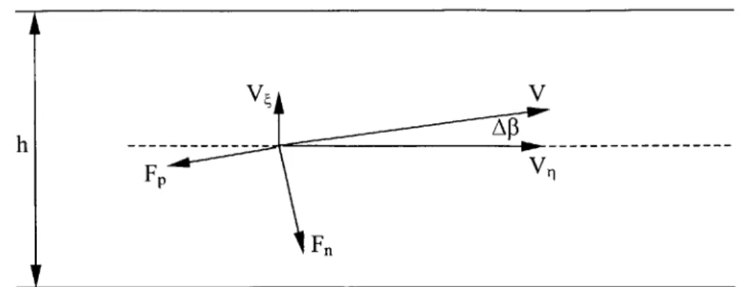
A key aspect of the formulation is to express the body force as a function of local flow properties. To elucidate the functional dependency of body force on local flow properties, it is useful to examine flow in a straight channel which is, in a first order approximation, similar to flow in a blade passage. A sector of a blade passage is considered as a straight channel, and the flow properties at a particular location are indicated in Fig. 2.2.

Vg V

h

Fp Vq

Fn

Fig. 2.2 Flow in a blade passage is modeled locally as a flow in a straight channel The force can be expressed as

hF (.0

V2 _{= f(M, Ap, Re) (2.10)}

where V, M, Ap and Re are local velocity, mach number, relative flow angle and Reynolds number respectively. h is the local spacing of the blade passage. For high enough Re, the viscous effect is negligible, therefore an adequate form of the body force is

hF

V2 ₌

_f(M,

Following the analysis of Marble, it is useful to split the body force into two parts: one normal to the relative flow direction annotated as Fn, the other parallel to the flow direction in the relative frame. An advantage of splitting the body force representation into these two parts is that each part can be formulated on its own physical meaning. Fn represents the effects of pressure difference between the pressure surface and suction surface, which enables work exchange between fluid and blade row. The body force parallel to the flow, Fp, is due to the viscous shear stress. The functional dependence of the body force can be written as

hF -- ";

f,

f,

The pressure gradient in a staggered channel could also produce pressure difference across the blade, as shown in Fig. 2.3. The pressure gradient in a staggered blade passage is different from the axisymmetric assumption which states that the pressure gradient is in the direction of the meridional plane. The force term which corresponds to the local pressure gradient is 1lap. F = sina (2.14) p ax V - ''P2 ---- Fn x PI P3 ,P -P "ph

Fig. 2.3 Body force due to pressure gradient in a staggered channel. The velocity is along the blade passage; and the pressure gradient is also in the blade passage direction. The pressure gradient has a component in circumferential direction, so it creates the pressure

difference (P3-P1) across the blade.

2.2.2 Body Force Formulation Proposed in Gong [9]

The formulation proposed in Gong [9] yield a body force that represents the blade response to the discrepancy between blade metal angle and flow direction. The flow in a blade passage is locally modeled as flow in a straight channel, as shown in Fig. 2.3 11 and

4 are the axes in the local blade channel direction and the direction normal to the local blade channel respectively.

aV,

Vqr/= (2.15)

Therefore, the normal to blade passage component of the normal body force has the following form

V7V

h (2.16)

In the above expression, h is preferred to the blade chord since h can be defined locally. Using the functional form of Eq. 6.4, the F can be expressed as

V V

F, = K,q(Af, M) 7h

h (2.17)

An undesirable difficulty associated with above formulation is when Ap8 reaches 900

(2.18)

v 2

F = F,, tan(Ap8) = K(ApM)

h

which has a finite value. This can not be right since F, , must be zero in this situation. To overcome this, the formulation is modified to:

(2.19)

=K(Ap,8,M) 1

h

The above form is nearly equivalent to the original form when Ap8 is small since

F, = cos ApiF (2.20)

and it will not be zero if V, becomes zero.

Upon applying the above formulation in a blade passage where the local blade passage (a straight channel) is along the local blade metal angle, a , we have

F, = Fn sin(a + Ap8)n, =

F =-Fn~ cos(a + A/8)

(2.21) (2.22) The final results of normal body force can be written as:

F, =K (A "M) (V, cos a + V sin a)(V

h V

F, = K, (Ap, M) Vx (Vx cos a + V9 sin a)(V

h V cos a - V, sin a) cos a - V, sin a) (2.23) (2.24) F,g

The expressions for viscous shear force is against the flow direction, and can be written as FPX _{K (AP,M)} h F =K (A#3,M) Fp =- h VV6 (2.25) h F' K,(A#, M) p~r h

Where K is the parallel body force coefficient. The resultant parallel body force is the vector sum of all these terms.

A significant feature of the current body force representation is that it is a function of local flow properties. This is essential to model non-linear three-dimensional disturbances in compressors where flow redistribution occurs in a blade row in the presence of these disturbances.

2.3 Numerical method

The governing equations of this body force formulation are three-dimensional unsteady Euler equations. The solution procedure for the governing equations for the compressor model is based on a standard finite volume discretization and a multi-stage Runge-Kutta method for time discretization [22].

The flows within blade row and duct regions are compatible with one another in the computational domain. This will be demonstrated in the following. Fig. 2.4 shows the fluxes through a computational cell in the blade row region. The role of blades is to block (or force) the fluxes through the constant 0 face (in the shadowed area). More specifically, if the cell is in a stator blade row, there is no flux through that face, and if

8

the cell is in a rotor blade row, the flux is evaluated using a U. The term can be

ao

viewed as the mass and momentum that are forced into the cell by the moving blades. The fluxes on the other faces can be evaluated in the way used by Jameson [22]. The interface between blade row region and duct region is the constant r face; the fluxes on

that face can be evaluated by the same method as is for the three-dimensional flow region. Thus coupling the two types of flow region will not cause any incompatibility problem.

Infinite number of blades block flow through them

Normal fluxes on these faces

Ar K

Xl

x

Fluxes on this face are only caused by moving blades

Fig. 2.4 Illustration of fluxes evaluation around a cell in the blade row region

The inlet and exit boundary conditions are standard one-dimensional linearized boundary conditions [28]. The exit static pressure of the computational domain is updated every iteration using the plenum-throttle equation.

2.4 Summary

The non-linear three-dimensional computational model for high-speed compressors which was developed in Gong [9] has been introduced and briefly summarized in this chapter. The key aspect of the model is to emphasize the three-dimensional compressor blade row response to general three-dimensional non-linear flow disturbances. The model has proved to be adequate in simulating compressor response to different types of inlet distortions in Gong [9]. However, its adequacy has not been assessed in terms of

capturing the instability behavior in high-speed compressors, this motivates and constitutes the main work of chapter 3.

Chapter 3

Instability Calculation of a High-Speed Compressor

In this chapter, the computational model for high-speed compressors presented in Chapter 2 is used to simulate the instability behavior of a high-speed single stage compressor (NASA stage-35 compressor) for both clean inlet flow and inlet distorted flow. The work is mainly aimed at assessing the adequacy of the computational model in [9] for

simulating the instability behavior in high-speed compressors.

This chapter is arranged as follows: Section 1 briefly introduces the research compressor. Section 2 shows the instability calculation results using the body force formulation in Gong [9]. Section 3 compares the computational results with the experiment; the observed discrepancies between the computational results and experimental observation are delineated to provide motivation for the work described in chapter 4. Section 4 gives a summary of this chapter.

3.1 NASA Stage 35 Compressor

NASA Stage 35 is a single stage transonic compressor designed by NASA Glenn Research Center in the late 70's [12]. The compressor features low aspect ratio rotor and stator blades and a high design pressure ratio of 1.82. The design parameters are listed in Table 3.1. The rotor and stator of this compressor are shown in Fig. 3.1.

C-77-677 Rotor

Stator

Number of rotor blades 36 Rotor rotating speed 1800 rad/sec

Rotor aspect ratio 1.19

Hub-to-tip ratio at rotor inlet 0.7 Solidity of rotor 1.29 at tip

1.77 at hub

Number of stator blades 46

Stator aspect ratio 1.26

Solidity of stator 1.3 at the tip

1.5 at the hub Table 3.1 Design parameters of Stage 35 Compressor The computational domain is shown in Fig. 3.2

upstream

_{inlet exit}

*

I

downstream

Fig. 3.2 Computational domain of NASA stage 35 compressor

The only difference between the configuration shown and actual experimental configuration setup is that near the exit, the flow path has been modified to avoid any numerical difficulties due to reverse flow at the hub-wall curvature (shown by dashed line). Fig. 3.3 and Fig. 3.4 show the computational mesh in meridional plane and compressor inlet face respectively.