HAL Id: hal-02275922
https://hal.archives-ouvertes.fr/hal-02275922
Submitted on 18 Feb 2021
HAL is a multi-disciplinary open access
archive for the deposit and dissemination of
sci-entific research documents, whether they are
pub-lished or not. The documents may come from
teaching and research institutions in France or
abroad, or from public or private research centers.
L’archive ouverte pluridisciplinaire HAL, est
destinée au dépôt et à la diffusion de documents
scientifiques de niveau recherche, publiés ou non,
émanant des établissements d’enseignement et de
recherche français ou étrangers, des laboratoires
publics ou privés.
pair-matching of long bone antimeres: An evaluation on
modern and archaeological samples
Frédéric Santos, Sébastien Villotte
To cite this version:
Frédéric Santos, Sébastien Villotte.
Using quadratic discriminant analysis for osteometric
pair-matching of long bone antimeres: An evaluation on modern and archaeological samples. International
Journal of Osteoarchaeology, Wiley, 2019, �10.1002/oa.2815�. �hal-02275922�
For Peer Review
Using quadratic discriminant analysis for osteometric
pair-matching of long bone antimeres: An evaluation on modern
and archaeological samples
Journal: International Journal of Osteoarchaeology Manuscript ID OA-19-0070.R1Wiley - Manuscript type: Research Article Date Submitted by the
Author: n/a
Complete List of Authors: Santos, Frédéric; CNRS – Université de Bordeaux – MCC, UMR 5199 PACEA
Villotte, Sébastien; CNRS – Université de Bordeaux – MCC, UMR 5199 PACEA
For Peer Review
DOI: xxx/xxxx
RESEARCH ARTICLE
Using quadratic discriminant analysis for osteometric
pair-matching of long bone antimeres: An evaluation on modern
and archaeological samples
Frédéric Santos | Sébastien Villotte
Université de Bordeaux — CNRS — MCC, UMR 5199 PACEA, 33600 Pessac, France
Correspondence
Frédéric Santos, Université de Bordeaux, UMR 5199 PACEA, Bâtiment B8, Allée Geoffroy Saint-Hilaire, CS 50023, 33615 Pessac Cedex, France. Email: [email protected]
Abstract
A common problem in forensic anthropology is the pair-matching of left and right bone antimeres. Several osteometric sorting models have been proposed in the last 20 years, with a recent acceleration in new methodological articles bringing sometimes contradictory results or recom-mendations. These debates demonstrate the need for a statistical tool both accurate and easily applicable by the final user.
We present here an approach based on quadratic discriminant analysis (QDA). This approach is evaluated on antimeric pairs of humeri and femora from the openly available Goldman Data Set, and compared to two classical and previously published methods for osteometric pair-matching, based respectively on linear regressions and t-tests. It is shown that QDA globally outperforms existing solutions for reassociating those long bones, in particular by rejecting fewer true bone pairs at the classical α level of 0.10. The accuracy of all three methods is analyzed through receiver operating characteristic (ROC) curves to assess the influence of the choice of a decision threshold. The application on archaeological commingled remains of pair-matching models learned on a modern reference multipopulation sample is discussed. Finally, an R package containing the func-tions used for this study, bonepairs, is publicly available online. This ensures the full replicability of results and an easy use of the new method introduced here.
KEYWORDS:
commingled remains, forensic anthropology, linear regression, osteometric sorting, paired ele-ments, QDA, R language, ROC curves
1
INTRODUCTION
Discoveries of commingled human skeletal remains are frequent in both forensic and archaeological contexts, and getting reliable individual data from these assemblages is considerably harder than when anatomical connections can be recorded in the field. Classically in these cases, archae-ologists and forensic anthroparchae-ologists attempt to find what was called by Villena Mota, Duday, and Houët (1996) “liaisons ostéologiques de second ordre”, by looking in laboratory for bone associations not recorded in the field, mostly attempting to find pairs of bones or articular congruence between two or three bones. However this approach is both time consuming and very subjective. Other methods can be applied, including the interbone comparisons of DNA (e.g. Čakar et al. 2018), bone weight (Baker & Newman 1957), ultraviolet fluorescence (Eyman 1965), taphonom-ical alterations (Kerley 1972) and osteometrics (e.g. Byrd & LeGarde 2014). This paper focuses on the last approach, and more specifically on pair-matching—i.e. the study of left and right antimeres— of femora and humeri.
1
2
3
4
5
6
7
8
9
10
11
12
13
14
15
16
17
18
19
20
21
22
23
24
25
26
27
28
29
30
31
32
33
34
35
36
37
38
39
40
41
42
43
44
45
46
47
48
49
50
51
52
53
54
55
56
57
For Peer Review
Osteometric sorting is an active research topic in forensic anthropology. Numerous theoretical articles have recently been published to propose new methods or refinements of previous methods (e.g., Lee & Konigsberg 2018; Lynch 2018b; Warnke-Sommer, Lynch, Pawaskar, & Damann 2019), although “few studies have been conducted to validate these proposed methologies” as noted by Bertsatos and Chovalopoulou (2019, p. 257–258).
This study has two main goals. First, a new statistical technique for osteometric pair-matching based on quadratic discriminant analysis (QDA) is described. This method is tested against two classical methods: Lynch’s revised version of Byrd’s (Byrd 2008; Byrd & LeGarde 2014) osteometric sorting model based ont-tests (Lynch, Byrd, & LeGarde 2018), and a method based on prediction intervals of linear regressions (Adams & Byrd 2006; Byrd & Adams 2003). The latter is traditionally used to reassociate two different bone portions but is also applicable to pair-matching. We follow the instructions recently described by Byrd and LeGarde (2018) for proper statistical comparison of all methods by reporting adequate indicators. The second goal is to continue the discussion initiated by Bertsatos and Chovalopoulou (2019) for the applicability of osteometric sorting models on archaeological samples when no reference sample from the past population is available. In such a case, a modern sample is used as learning dataset to train the statistical models, and those models are then applied on the archaeological sample. It has long been noted that the learning and test samples must be comparable for this procedure to perform well (Byrd & LeGarde 2014), but this is rarely the case. This problem can hardly be circumvented; however it is possible to search for a statistical method which could exhibit a better robustness in such a situation. The three methods under study are compared using a modern reference sample and four archaeological test samples, and taking into account the multipopulational origin of the reference sample.
2
MATERIALS AND METHODS
2.1
Samples and measurements
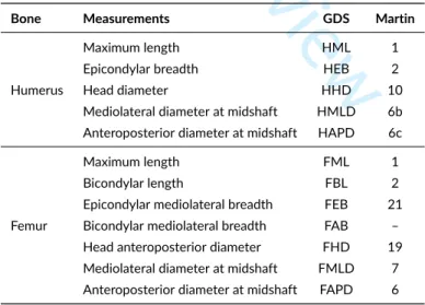
The Goldman Data Set (Auerbach & Ruff 2004), publicly available online in CSV (comma-separated values) format, is the core material of this study. This dataset consists of osteometric measurements taken from 1538 human skeletons in total. To simplify the demonstration, this study focuses on pair-matching for left and right antimeres of humeri and femora. The measurements available in this dataset for these two bones are indicated in Table 1 .
TABLE 1 Linear measurements used for the humerus and femur. Their corresponding shortcodes in the Goldman Data Set (GDS, Auerbach & Ruff
2004) and R. Martin (1928) are indicated.
Bone Measurements GDS Martin
Humerus
Maximum length HML 1
Epicondylar breadth HEB 2
Head diameter HHD 10
Mediolateral diameter at midshaft HMLD 6b Anteroposterior diameter at midshaft HAPD 6c
Femur
Maximum length FML 1
Bicondylar length FBL 2
Epicondylar mediolateral breadth FEB 21 Bicondylar mediolateral breadth FAB – Head anteroposterior diameter FHD 19 Mediolateral diameter at midshaft FMLD 7 Anteroposterior diameter at midshaft FAPD 6
Using the Goldman Data Set presents two main advantages. First, almost all recent studies utilize datasets that are not freely available—or only in part—, such as Jantz’s DFAUS (Jantz & Moore-Jansen 2006), Byrd and LeGarde’s reference dataset (Byrd & LeGarde 2014) or the reference dataset from the POW/MIA Accounting Agency (e.g., Lynch 2018b). Choosing the Goldman Data Set allows to replicate all the results from the present study with the R code made available on GitLab (https://gitlab.com/f.santos/ijoa-santos-villotte-2019).
1
2
3
4
5
6
7
8
9
10
11
12
13
14
15
16
17
18
19
20
21
22
23
24
25
26
27
28
29
30
31
32
33
34
35
36
37
38
39
40
41
42
43
44
45
46
47
48
49
50
51
52
53
54
55
56
57
For Peer Review
Second, the Goldman Data Set includes individuals from throughout the Holocene, thus allowing to select various subsamples corresponding to different periods, geographical origins and subsistence modes. Five main subsets of individuals extracted from this dataset are considered in this study: one modern sample, and four archaeological samples. The modern sample is composed of the individuals from the Hamann-Todd collection, a multipopulation sample covering Eastern and Western Europe; while the four archaeological samples include individuals all over the world.
The Goldman Data Set was inspected in search of clear outliers. The raw right-left differences were calculated for each individual on all mea-surements. The individuals exhibiting a raw difference greater than four times the interquartile range for any given measurement were excluded from the dataset. This rule, more permissive than the usual Tukey’s (1977) rule, does not aim at a drastic exclusion of extreme values, so that the removed cases are likely to be due to either entry error, strong measurement error or life-history related idiosyncrasy of a given individual. The few other individuals with slightly unusual asymmetries were left in on purpose, all of their asymmetries being considered as biologically plausible. In total, five pairs of humeri and three pairs of femora were excluded from the total sample according to this rule.
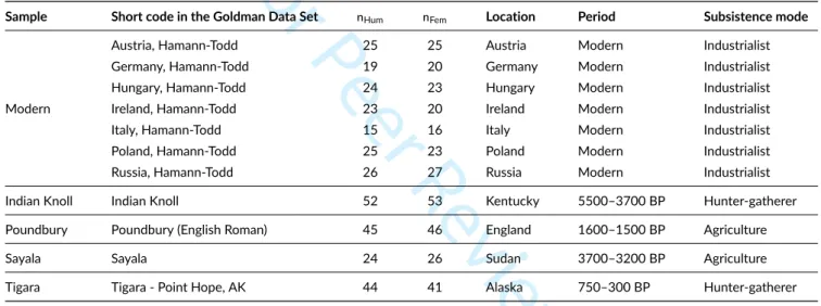
A summary of the five samples under study—after excluding the outliers—can be found on Table 2 .
TABLE 2 Detailed composition of the five samples utilized in this study. All population samples are drawn from the Goldman Data Set (Auerbach
& Ruff 2004), and their corresponding short code is given.nHum: number of individuals having all left and right humeral measurements presented
in Table 1 ;nFem: number of individuals having all left and right femoral measurements presented in Table 1 . All information about location,
chronological period and subsistence mode are extracted from the Goldman Data Set online documentation.
Sample Short code in the Goldman Data Set nHum nFem Location Period Subsistence mode
Modern
Austria, Hamann-Todd 25 25 Austria Modern Industrialist
Germany, Hamann-Todd 19 20 Germany Modern Industrialist
Hungary, Hamann-Todd 24 23 Hungary Modern Industrialist
Ireland, Hamann-Todd 23 20 Ireland Modern Industrialist
Italy, Hamann-Todd 15 16 Italy Modern Industrialist
Poland, Hamann-Todd 25 23 Poland Modern Industrialist
Russia, Hamann-Todd 26 27 Russia Modern Industrialist
Indian Knoll Indian Knoll 52 53 Kentucky 5500–3700 BP Hunter-gatherer
Poundbury Poundbury (English Roman) 45 46 England 1600–1500 BP Agriculture
Sayala Sayala 24 26 Sudan 3700–3200 BP Agriculture
Tigara Tigara - Point Hope, AK 44 41 Alaska 750–300 BP Hunter-gatherer
2.2
Inspection of asymmetry
The reference modern sample and the four archaeological samples may present asymmetries that differ in a substantial manner. Thus, a careful inspection of the patterns of asymmetry—and in particular directional asymmetry if it exists—is essential to allow further discussion about the applicability on past populations of models learned on a modern sample.
We then performed exploratory analyses to evaluate the differences in asymmetries among all samples. First, to compare the multivariate asymmetry patterns among groups, a principal component analysis (PCA) was computed on the matrix of raw right-left differences of measurements for all individuals, using the R packageFactoMineR (Lê, Josse, & Husson 2008). The variables were all scaled to unit variance beforehand. Second, to evaluate the level of asymmetry of each measurement in each population sample, medians of percentage directional (%DA) and absolute (%AA) asymmetry—e.g. as defined in Auerbach and Ruff (2006)—were calculated.
2.3
Study design
First, the three statistical methods under study are evaluated when considering all available measurements for each bone. In a second time, the methods are evaluated when using only a subset of measurements. In the latter case, three out of the five humeral measurements (HHD, HAML
1
2
3
4
5
6
7
8
9
10
11
12
13
14
15
16
17
18
19
20
21
22
23
24
25
26
27
28
29
30
31
32
33
34
35
36
37
38
39
40
41
42
43
44
45
46
47
48
49
50
51
52
53
54
55
56
57
For Peer Review
and HAPD), and four out of the seven femoral measurements (FEB, FAB, FMLD, FAPD) are used. The goal was primarily to assess the influence of maximum lengths, by considering theoretical cases where an extremity (distal end of humerus, or proximal end of femur) is damaged. This situation, frequently encountered in archaeological remains, prevents to measure accurately the maximum length and the damaged extremity, while the location of the midshaft can still be identified, allowing to measure the mediolateral and anteroposterior diameters.
The evaluation of the three pair-matching methods for a given bone (femur or humerus) and a given set of measurements proceeds through the following steps.
Step 1. Filter the five samples under study to discard the individuals having at least one missing value among the considered measurements. The
number of remaining individuals can be found in Table 2 .
Step 2. The multipopulation modern sample includes people from seven European countries. Even if one can consider that they are closely related,
not taking into account those multiple origins may lead to an erroneous increase in classification accuracy on the learning sample. Indeed, the exclusion of bone pairs coming from two populations that differ in stature or body proportions is easier to achieve, and may not reveal the true efficiency of a pair-matching method in real cases. Thus, it was decided to consider only the bone pairs within each of the seven countries from the modern multipopulation sample, so that two bones originating from two different countries will never be compared. This approach also fits the archaeological sense since the question of pair-matching of two bones coming from different sites or collections is never of practical interest. Thus, two lists of possible bone associations are created. The first one is the list of all the true pairs of skeletal elements (i.e., if there arenindividuals in total in the modern sample, thenntrue bone pairs can be listed). The second one is a list of “false associations” (i.e. bone pairs that belong to distinct individuals) within each country from the modern sample. All the country-specific lists of false associations are then concatenated to create a global list of false bone associations in the modern sample. Consequently, the association of a left bone coming—for instance—from Austria with a right bone coming from Germany is never tested; but the association of all left and right bones originating from each single given country is exhaustively evaluated. In summary, if there arenindividuals coming fromKdifferent countries,ntrue bone pairs andřK
i“1n2i “false associations” are considered, whereniis the number of individuals coming
from thei-th country.
Step 3. The three statistical methods described below use the modern sample as a learning dataset, and their accuracies are evaluated using a
leave-one-out cross-validation (LOOCV) on all the—true or false—bone pairs made available from this sample.
Step 4. The three models learned on the modern sample are then applied on all possible pairs of elements from each archaeological sample, thus
allowing to evaluate exhaustively their applicability on assemblages from other geographical origins and chronological periods.
By convention, a “positive” outcome for a given pair of bone is the rejection of the hypothesis that the two bones belong to the same individual; and a “negative” outcome is the failure to reject this hypothesis. In accordance to Byrd and LeGarde’s (2018) recommendations, the performance of the three methods is evaluated by reporting the true positive rate (TPR), i.e. the percentage of bones that were excluded by the statistical model and were true exclusions:
TPR“ TP
TP`FN (1)
where TP is the number of true positives (correct exclusions of bone pairs belonging to distinct individuals) and FN is the number of false negatives (failures to exclude bone pairs belonging to distinct individuals).
The false positive rate (FPR), i.e. the percentage of true bone pairs that are erroneously excluded, is also reported: FPR“ FP
FP`TN (2)
where FP is the number of false positives (erroneous exclusions of bone pairs that belong to the same individual) and TN is the number of true negatives (true bone pairs that were correctly not excluded).
Since all three statistical methods provide eitherp-values (linear regressions andt-tests) or posterior probabilities (QDA) for the exclusion of a given pair of bones, the results can be reported at various confidence levels. Hereafter, the threshold used to reject a bone association will be called “αlevel”. Byrd recommends choosing anαlevel of 0.10 as a good compromise for linear regressions andt-tests (Byrd & LeGarde 2014). Thus, detailed results are given at this threshold for the three methods: for linear regressions andt-tests, a bone association will be rejected if its associatedp-value is less than 0.10, and for QDA, if the associated posterior probability for the class “this pair may belong to the same individual” is less than 0.10.
However, other choices ofαlevels can also be reasonable depending on the context of the study (Lynch 2018a). To facilitate the comparisons of the three methods independently of theαlevel chosen, receiver operating characteristic (ROC) curves can be used (Fawcett 2006). A ROC curve plots the TPR against the FPR at variousαlevels, and provides a synthetic score of classification accuracy: the AUC (area under the curve). Ranging
1
2
3
4
5
6
7
8
9
10
11
12
13
14
15
16
17
18
19
20
21
22
23
24
25
26
27
28
29
30
31
32
33
34
35
36
37
38
39
40
41
42
43
44
45
46
47
48
49
50
51
52
53
54
55
56
57
For Peer Review
from 0.50 (no better accuracy than chance alone) to 1 (perfect accuracy), the AUC offers an easy way to compare several models. The closer a ROC curve reaches to the top left corner, the better the accuracy. The ROC curves presented here were computed using thepROC R package (Robin et al. 2011). When necessary, the best possibleαlevel for each method was determined using the Youden’sJindex (Youden 1950).
In real case studies, ROC analyses cannot be performed on the archaeological commingled remains since the “true” status (“belongs to the same individual” / “does not belong to the same individual”) of each possible bone pair is not known. To fit with archaeological sense, we performed here ROC analyses using the results obtained in LOOCV on the modern reference sample. Aiming to find the bestαvalue for a given archaeological dataset after the analysis of a modern training set is the only feasible way to proceed, however it may lead to unsatisfactory results. The relevance of this approach will be discussed for the three methods of pair-matching.
All the calculations were done using R 3.6.1 (R Core Team 2019), and each of the three methods below has been implemented through an R function. All R functions written for this analysis are publicly available as an R package,bonepairs, that can be installed from a GitLab repository (http://gitlab.com/f.santos/bonepairs). The R code making use ofbonepairs for this case study is also available as a reproducibility package hosted on GitLab (https://gitlab.com/f.santos/ijoa-santos-villotte-2019).
2.4
Methods evaluated
2.4.1 Lynch’s revised pair-matching model based on t-tests
This method is derived from Byrd’s osteometric sorting model (Byrd 2008; Byrd & LeGarde 2014) based ont-tests. It has been proven to bring a significant improvement to the original model (Lynch et al. 2018; Warnke-Sommer et al. 2019).
The variant evaluated here calculates aDvalue for each true bone pair in the learning sample:
D “ ˜ 0.00005 `ÿ i |li´ ri| ¸λ (3) whereliis thei-th left measurement andriis thei-th right measurement from the considered bone pair, andλis a parameter for Box-Cox
transformation.
To study the association of a given bone pair, at-statistic is computed:
t “Dobs´ D
ˆ σD
(4) whereDobsis the observedDvalue for the bone pair under study,Dis the mean of allDvalues computed in the reference sample, andσˆDtheir
standard deviation. In this model, the null hypothesis is that a given bone pair belongs to the same individual. Thetvalue is to be compared to a two-tailedt-distribution to produce ap-value.
The functionpm_lynch_auto() implements this method in the R packagebonepairs. It has been tested to be consistent with—and is essentially derived from—Lynch’spm.ttest function, implemented in his R packageOsteoSort (Lynch 2019). Our implementation inbonepairs takes into account a suggestion from Lee and Konigsberg (2018) about the choice of theλparameter for Box-Cox transformation. Instead of setting this exponent to a given value from the literature (usually 0.33), a maximum likelihood method is used to find the best possible value in each case.
2.4.2 Byrd and Adams’ method based on linear regressions
This model defined by Byrd and Adams (Adams & Byrd 2006; Byrd & Adams 2003) is widely used through the literature for reassociating distinct bone portions, but seems to never have been evaluated for the case of pair-matching.
In this method, the following values are calculated for each true pair of bones :
L “ logpÿ i liq (5) R “ logpÿ i riq (6)
whereliandriare thei-th left and right measurements for the bones considered. A simple linear regression is then build between allLandR
values, e.g. withRas dependent variable andLas independent variable.
Then, for any given new pair of bones, the followingt-value is calculated (Byrd & LeGarde 2014):
t “ | ˆRn`1´ Rn`1| ˆ σ b 1 ` 1{N ` pLi´ ¯Lq2{pnˆσ2Lq (7)
1
2
3
4
5
6
7
8
9
10
11
12
13
14
15
16
17
18
19
20
21
22
23
24
25
26
27
28
29
30
31
32
33
34
35
36
37
38
39
40
41
42
43
44
45
46
47
48
49
50
51
52
53
54
55
56
57
For Peer Review
whereRˆn`1is the predicted value by the regression model of the considered pair,Rn`1is its real dependent (right) value,σˆis the regression
model residual standard error,nis the number of true bone pairs used in calculation of the regression model,Liis the independent (left) value of
the considered pair,L¯is the reference sample mean for theLvalues, andˆσ2
Lis the reference sample variance of theLvalues.
As in the previous model, the null hypothesis is that a given bone pair belong to the same individual. Thetvalue is to be compared to a two-tailed
t-distribution to produce ap-value.
The functionpm_logreg_auto() implements this method in the R packagebonepairs.
2.4.3 Quadratic discriminant analysis
Quadratic discriminant analysis (QDA) is a classifier closely related to Fisher’s linear discriminant analysis (Fisher 1936). QDA allows to find an efficient decision rule when a linear discriminant procedure is not sufficient to separate the groups under study, or when the covariance matrices are not equal among groups (Rencher & Christensen 2012).
In this approach we first compute, for all—true or false—bone pairs made available from the reference sample, all differences between left and right measurements. A dataset is then obtained, with one row per bone pair, and one column per left-right difference in bone measurements. In the next step, a QDA model is learned on this dataset with all raw left-right differences as predictors, the response variable being the binary information “this pair of bones belongs to a single individual / this pair of bones comes from two distinct individuals”. QDA delivers posterior probabilities for these two classes, thus allowing to set anαlevel as in previous methods: a bone pair will be classified as coming from distinct individuals if the probability that it belongs to the same individual is lower than a given thresholdα.
The R functionpm_qda_auto() implements this procedure in the R packagebonepairs, and the computation of QDA models in this function relies on the R packageMASS (Venables & Ripley 2002). Equal priors (0.5, 0.5) were given to the classes “this pair of bones belongs to a single individual / this pair of bones comes from two distinct individuals” in this study, but custom priors are allowed in the R function.
The variability in left-right differences for the bone pairs that belong to distinct individuals is expected to be much higher than the variability for the bone pairs that belong to one single individual. In other words, the generalized variance of the differences in left-right measurements—i.e. the determinant of their covariance matrix (Wilks 1960)—should differ very substantially between the two classes under study, thus invalidating the hypothesis of equality of covariance matrices required by LDA. This is the rationale behind the choice of QDA rather than the classical LDA in this study (James, Witten, Hastie, & Tibshirani 2013). An R code proving the inequality of covariance matrices in a formal way is available as Supporting Information online (Appendix S2).
3
RESULTS
3.1
Pair-matching of humeri
First, the asymmetry of humeral measurements within the five samples under study was inspected. The principal component analysis (PCA) per-formed on raw right-left differences of all humeral measurements is presented in Figure 1 . Global patterns of asymmetry differ substantially from one sample to another. The PCA suggests that individuals from Indian Knoll exhibit a stronger asymmetry for the anteroposterior midshaft diam-eter (HAPD), which is confirmed by a higher observed %DA for this measurement in this sample (Table 3 ). Poundbury sample exhibits a stronger asymmetry on the humerus maximum length (HML) as shown on Figure 1 and Table 3 . Contrarily, the modern multipopulation sample and the agricultural population sample of Sayala do not exhibit strong directional asymmetries.
The three methods of pair-matching were then applied on the modern sample, and these models were used to predict the bone associations on the four archaeological samples. When all five humeral measurements are considered, the results given at anαlevel of 0.10 are presented in Table 4 . In the modern learning sample, no difference in false positive rate and a limited difference in true positive rate can be observed between the two classical methods—t-tests and linear regressions. As expected when setting anαlevel of 0.10, their false positive rates are close to 10%. Conversely, QDA clearly outperforms the existing methods in both TPR and FPR, and falsely rejects as much as ten times less true bone pairs (1.3 %) at thisαlevel. This trend is confirmed on the archaeological samples: at this cut-off value, QDA always delivers better true positive rates, and much lower false positive rates—except for Sayala sample—than the existing methods.
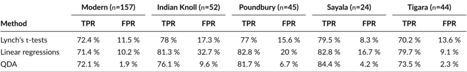
The same analyses using only three out of the five available humeral measurements (HHD, HMLD and HAPD) were performed. The results, still given at anαlevel of 0.10, are presented in Table 5 . In this case, all the true positive rates are strongly reduced compared to the previous
1
2
3
4
5
6
7
8
9
10
11
12
13
14
15
16
17
18
19
20
21
22
23
24
25
26
27
28
29
30
31
32
33
34
35
36
37
38
39
40
41
42
43
44
45
46
47
48
49
50
51
52
53
54
55
56
57
For Peer Review
−6 −4 −2 0 2 4 6 −4 −2 0 2 4Individuals factor map (PCA)
Dim 1 (28.11%) Dim 2 (25.79%) Indian Knoll Modern Poundbury Sayala Tigara −1.0 −0.5 0.0 0.5 1.0 −1.0 −0.5 0.0 0.5 1.0
Variables factor map (PCA)
Dim 1 (28.11%) Dim 2 (25.79%) HML HEB HHD HMLD HAPD
FIGURE 1 Principal component analysis on raw right-left differences of humeral measurements presented in Table 1 including the five samples
under study. Group centroids are represented by stars (“*”).
TABLE 3 Medians of percentage directional asymmetry (%DA) and absolute asymmetry (%AA) of humeral measurements in each sample considered
in this study. The results are given in the format %DA / %AA.
Sample HML HEB HHD HMLD HAPD
Modern 1.08% / 1.15% 1.57% / 1.68% 0.19% / 1.3% 0.1% / 2.46% 5.59% / 5.59% Indian Knoll 1.09% / 1.24% 2.27% / 2.61% 0.38% / 1.33% 4.97% / 5.32% 10.73% / 10.73% Poundbury 2.39% / 2.39% 1.55% / 1.83% 0% / 1.79% 3.94% / 4.06% -1.25% / 2.45% Sayala 1.34% / 1.34% 0% / 1.59% 1.12% / 1.43% 3.62% / 4.84% -0.23% / 2.39% Tigara 2.25% / 2.25% 0.43% / 1.94% 0.41% / 1.85% 1.52% / 1.94% 2.13% / 3.16%
TABLE 4 Results of the three statistical methods for the pair-matching of left and right humeri. The modern sample was used as the learning
dataset, and the models were then applied on the archaeological samples. Classification accuracy is expressed by TPR, true positive rate, and FPR, false positive rate. All five available measurements were used. The results are given at anαlevel of 0.10.
Modern (n=157) Indian Knoll (n=52) Poundbury (n=45) Sayala (n=24) Tigara (n=44)
Method TPR FPR TPR FPR TPR FPR TPR FPR TPR FPR
Lynch’st-tests 87.2 % 12.1 % 86.8 % 11.5 % 88.6 % 22.2 % 87.9 % 16.7 % 82.5 % 13.6 % Linear regressions 83.4 % 12.1 % 86.6 % 15.4 % 88 % 22.2 % 81.9 % 4.2 % 84 % 18.2 %
QDA 91 % 1.3 % 89.7 % 3.8 % 92.5 % 11.1 % 94.2 % 8.3 % 86.2 % 2.3 %
case, suggesting that the removal of maximum lengths leads to less efficient pair-matching models. In the modern sample, the three methods deliver roughly identical true positive rates, but QDA stands out by allowing about five times fewer false positives than classical methods (1.9 %, versus more than 10 % fort-tests and linear regressions). The false positive rates obtained witht-tests and linear regressions on the archaeological samples, although not systematically worse than when using all measurements, are up to 32.7 % and constantly at least twice as high as the FPRs
1
2
3
4
5
6
7
8
9
10
11
12
13
14
15
16
17
18
19
20
21
22
23
24
25
26
27
28
29
30
31
32
33
34
35
36
37
38
39
40
41
42
43
44
45
46
47
48
49
50
51
52
53
54
55
56
57
For Peer Review
TABLE 5 Results of the three statistical methods for the pair-matching of left and right humeri. The modern sample was used as the learning
dataset, and the models were then applied on the archaeological samples. Classification accuracy is expressed by TPR, true positive rate, and FPR, false positive rate. Only three out the five available measurements were used: HHB, HMLD and HAPD. The results are given at anαlevel of 0.10.
Modern (n=157) Indian Knoll (n=52) Poundbury (n=45) Sayala (n=24) Tigara (n=44)
Method TPR FPR TPR FPR TPR FPR TPR FPR TPR FPR
Lynch’st-tests 72.4 % 11.5 % 78 % 17.3 % 77 % 15.6 % 79.5 % 8.3 % 70.2 % 13.6 % Linear regressions 71.4 % 10.2 % 81.3 % 32.7 % 82.8 % 20 % 82.8 % 16.7 % 79.7 % 9.1 %
QDA 72.1 % 1.9 % 76.1 % 9.6 % 81.7 % 6.7 % 84.4 % 4.2 % 73.5 % 2.3 %
obtained with QDA. In addition to producing much fewer false positives, QDA also maintains a satisfactory ability to detect the true positives at thisαlevel, with true positive rates equivalent or greater than Lynch’st-tests for all four archaeological samples.
Humerus, modern sample (all measurements)
FPR (1−Specificity) TPR (Sensitivity) 0.0 0.2 0.4 0.6 0.8 1.0 0.0 0.2 0.4 0.6 0.8 1.0
Lynch’s t−tests AUC = 0.942 Linear regressions AUC = 0.919 QDA AUC = 0.987 0.01 0.05 0.1 0.25 0.5 0.01 0.05 0.1 0.25 0.5 0.01 0.05 0.10.25 0.5
(a) All humeral measurements are used
Humerus, modern sample (HHD, HMLD, HAPD)
FPR (1−Specificity) TPR (Sensitivity) 0.0 0.2 0.4 0.6 0.8 1.0 0.0 0.2 0.4 0.6 0.8 1.0
Lynch’s t−tests AUC = 0.877 Linear regressions AUC = 0.868 QDA AUC = 0.94 0.01 0.05 0.1 0.25 0.5 0.01 0.05 0.1 0.25 0.5 0.010.05 0.1 0.25 0.5
(b) Three out of five humeral measurements are used FIGURE 2 ROC analyses of the three pair-matching methods based on LOOCV applied on the modern sample. The results obtained at some
interestingαlevels (ranging from 0.01 to 0.50) are indicated on each curve by labeled dots.
The ROC analysis performed on the results obtained in LOOCV on the modern sample when all five measurements are considered (Fig. 2 a) indicates that QDA globally outperforms the existing methods for a wide range ofαlevels, thus leading to a better area under the curve (AUC). Additionally, for each possibleαlevel indicated on the plot, QDA exhibits both a better FPR and a better TPR than existing methods. A ROC analysis was also performed on the results obtained with only three humeral measurements (Fig. 2 b). For all theαlevels displayed on the plot, QDA exhibits a substantially better FPR and a roughly equivalent or slightly inferior TPR than classical methods.
1
2
3
4
5
6
7
8
9
10
11
12
13
14
15
16
17
18
19
20
21
22
23
24
25
26
27
28
29
30
31
32
33
34
35
36
37
38
39
40
41
42
43
44
45
46
47
48
49
50
51
52
53
54
55
56
57
For Peer Review
3.2
Pair-matching of femora
A principal component analysis reveals that no substantial differences in asymmetry patterns can be found among population samples (Fig. 3 ). Extensive results for %DA and %AA are available as Supporting Information online (Table S1).
−5 0 5 −4 −2 0 2 4
Individuals factor map (PCA)
Dim 1 (29.04%) Dim 2 (20.18%) Indian Knoll Modern Poundbury Sayala Tigara −1.0 −0.5 0.0 0.5 1.0 −1.0 −0.5 0.0 0.5 1.0
Variables factor map (PCA)
Dim 1 (29.04%) Dim 2 (20.18%) FBLFML FEB FAB FHD FMLD FAPD
FIGURE 3 Principal component analysis on raw right-left differences of femoral measurements presented in Table 1 including the five samples
under study. Group centroids are represented by stars (“*”).
Classification results when using all seven femoral measurements are presented in Table 6 . In the modern learning sample, QDA exhibits both a better TPR and FPR than the existing methods. The highest TPRs for all archaeological samples are also obtained with QDA, with an improvement ranging from 2.7 % to 7.7 % compared to Lynch’st-tests. The false positive rates obtained with QDA range from 0 % to 6.5 %, while the ones obtained with Lynch’st-tests are up to 14.6 % in Tigara sample. However, Lynch’st-tests deliver slightly better FPRs than QDA in two archaeological samples, Indian Knoll and Poundbury, although this difference relies on one single pair of femora. According to the AUC obtained through a ROC analysis, QDA still outperforms the existing methods for a wide range ofαlevels (Fig. 4 a).
TABLE 6 Results of the three statistical methods for the pair-matching of left and right femora. The modern sample was used as the learning
dataset, and the models were then applied on the archaeological samples. Classification accuracy is expressed by TPR, true positive rate, and FPR, false positive rate. All seven available measurements were used. The results are given at anαlevel of 0.10.
Modern (n=154) Indian Knoll (n=53) Poundbury (n=46) Sayala (n=26) Tigara (n=41)
Method TPR FPR TPR FPR TPR FPR TPR FPR TPR FPR Lynch’st-tests 89.4 % 8.4 % 88.8 % 0 % 91.4 % 4.3 % 90.5 % 3.8 % 88.1 % 14.6 % Linear regression 86.3 % 7.8 % 87.5 % 5.7 % 88.3 % 6.5 % 86.8 % 0 % 87.7 % 4.9 % QDA 93.6 % 3.2 % 92.9 % 1.9 % 96 % 6.5 % 98 % 0 % 90.9 % 4.9 %
1
2
3
4
5
6
7
8
9
10
11
12
13
14
15
16
17
18
19
20
21
22
23
24
25
26
27
28
29
30
31
32
33
34
35
36
37
38
39
40
41
42
43
44
45
46
47
48
49
50
51
52
53
54
55
56
57
For Peer Review
Femur, modern sample (all measurements)
FPR (1−Specificity) TPR (Sensitivity) 0.0 0.2 0.4 0.6 0.8 1.0 0.0 0.2 0.4 0.6 0.8 1.0
Lynch’s t−tests AUC = 0.954 Linear regressions AUC = 0.937 QDA AUC = 0.992 0.01 0.05 0.1 0.25 0.5 0.01 0.050.1 0.25 0.5 0.010.05 0.1 0.25 0.5
(a) All femoral measurements are used
Femur, modern sample (FEB, FAB, FMLD, FAPD)
FPR (1−Specificity) TPR (Sensitivity) 0.0 0.2 0.4 0.6 0.8 1.0 0.0 0.2 0.4 0.6 0.8 1.0
Lynch’s t−tests AUC = 0.926 Linear regressions AUC = 0.9 QDA AUC = 0.963 0.01 0.05 0.1 0.25 0.5 0.01 0.05 0.1 0.25 0.5 0.010.05 0.10.25 0.5
(b) Four out of seven femoral measurements are used FIGURE 4 ROC analyses of the three pair-matching methods based on LOOCV applied on the modern sample. The results obtained at some
interestingαlevels (ranging from 0.01 to 0.50) are indicated on each curve by labeled dots.
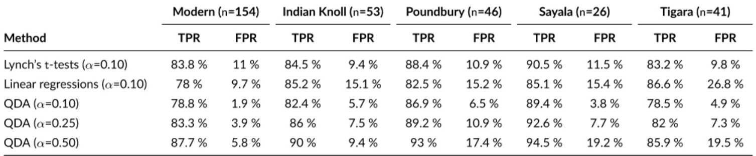
The same analyses were performed when using only four out of the seven available femoral measurements (FEB, FAB, FMLD, FAPD). The results are presented in Table 7 . At anαlevel of 0.10, QDA behaves constantly as a more prudential classifier than Lynch’st-tests by delivering both lower true positive rate and false positive rate, i.e. QDA seems to have less power to produce a positive (true or false) outcome at thisαlevel with this subset of measurements.
A ROC analysis was performed on the modern sample to explain this result (Fig. 4 b). According to Youden’sJindex (result not shown on the plot), the best possibleαlevels fort-tests and linear regressions are very close to 0.10 (respectively equal to 0.11 and 0.082), so that the results given at anαlevel of 0.10 are already nearly optimal for those two classical methods. Conversely, the best possible alpha level for QDA is equal to 0.50 according to Youden’sJindex, so that the results given at anαlevel of 0.10 are clearly sub-optimal for the modern sample. Thus, we added in Table 7 the results obtained for QDA using the best possibleαlevel according to Youden’sJindex (0.50), and an arbitrary intermediateαlevel (0.25). It appears that the optimal level of 0.50 indeed offers both a better TPR and FPR for QDA on the modern learning sample thant-tests and linear regressions. However, thisαlevel does not seem to be optimal for archaeological samples, since QDA allows way too many false positives on all four past populations (up to 19.5% in Tigara sample). The arbitrary intermediateαlevel of 0.25 gives more balanced results and offers a good compromise for archaeological samples, with both better TPR and FPR than classical methods in almost all cases.
4
DISCUSSION AND CONCLUSIONS
4.1
Comparison of the three methods under study
After Byrd’s (2008; 2014) recommendations, a dichotomy can be observed in the scientific literature depending on whether the aim is to reassociate the left and right antimeres of a given bone (pair-matching), or two different bone portions. Methods based on prediction intervals of linear models are generally used to reassociate two different bone portions (e.g., Adams & Byrd 2006; Anastopoulou, Karakostis, Borrini, & Moraitis 2018; Anastopoulou, Karakostis, & Moraitis 2019; Rodríguez, Hackman, Martínez, & Medina 2016). Although linear regressions are also applicable to antimeric bone pairs, Byrd’s (2008) osteometric sorting model based ont-tests —or any variation derived from this model— is always preferred in this case (e.g., Nikita & Lahr 2011). Most studies involving both pair-matching and study of different bone portions (e.g. Bertsatos & Chovalopoulou 2019; Rodríguez et al. 2016) also operate such a dichotomy by usingt-tests for pair-matching and linear regressions in all other situations. To the
1
2
3
4
5
6
7
8
9
10
11
12
13
14
15
16
17
18
19
20
21
22
23
24
25
26
27
28
29
30
31
32
33
34
35
36
37
38
39
40
41
42
43
44
45
46
47
48
49
50
51
52
53
54
55
56
57
For Peer Review
TABLE 7 Results of the three statistical methods for the pair-matching of left and right femora. The modern sample was used as the learning
dataset, and the models were then applied on the archaeological samples. Classification accuracy is expressed by TPR, true positive rate, and FPR, false positive rate. Four out of seven measurements were used (FEB, FAB, FMLD, FAPD). The results are given at specifiedαlevels.
Modern (n=154) Indian Knoll (n=53) Poundbury (n=46) Sayala (n=26) Tigara (n=41)
Method TPR FPR TPR FPR TPR FPR TPR FPR TPR FPR Lynch’st-tests (α=0.10) 83.8 % 11 % 84.5 % 9.4 % 88.4 % 10.9 % 90.5 % 11.5 % 83.2 % 9.8 % Linear regressions (α=0.10) 78 % 9.7 % 85.2 % 15.1 % 82.5 % 15.2 % 85.1 % 15.4 % 86.6 % 26.8 % QDA (α=0.10) 78.8 % 1.9 % 82.4 % 5.7 % 86.9 % 6.5 % 89.4 % 3.8 % 78.5 % 4.9 % QDA (α=0.25) 83.3 % 3.9 % 86 % 7.5 % 89.2 % 10.9 % 92.6 % 7.7 % 82 % 7.3 % QDA (α=0.50) 87.7 % 5.8 % 90 % 9.4 % 93 % 17.4 % 94.5 % 19.2 % 85.9 % 19.5 %
best of our knowledge, no study comparingt-tests and regression-based methods for pair-matching had been made to date on a large sample. The results presented here suggest that the particular statistical treatment reserved for the case of pair-matching was justified, sincet-tests globally outperform linear regression according to the classification results and ROC analyses obtained with the samples utilized in this study.
In a recent study, Vickers, Lubinski, Henebry DeLeon, and Bowen (2015) noted that, although false positives can be seen as more problematic than false negatives for archaeologists, the existing methods for osteometric sorting allow too many false rejections. From this point of view, using QDA—especially at the classicalαlevel of 0.10—is an attractive solution, guaranteeing that fewer true bone pairs will be wrongly rejected than with existing solutions, while maintaining a sufficient ability to detect the pairs belonging to distinct individuals (Tables 4 –7 ). However, Vickers et al.’s assertion has been nuanced by Byrd and LeGarde (2018, p. 347): “there is no good reason to optimize the test method to minimize the FP rate while ignoring other factors”. We agree that both parameters of classification accuracy—TPR and FPR—must be compared and that the best model should achieve the best compromise between them. Lynch’s osteometric sorting model based ont-tests offers high TPRs, is conceptually easy to understand and can be implemented using only a spreadsheet. For all these reasons, it remains a competitive solution for pair-matching, evaluated in numerous studies. However, according to the results of the present study, QDA outperforms this model in both parameters of classification accuracy when all measurements are available (Tables 4 and 6 ), and offers a more advantageous compromise—with substantially better FPR and roughly equivalent TPR—when fewer measurements are used (Tables 5 and 7 ).
4.2
Applicability in archaeological context
In archaeological contexts, commingled remains raise three main problems: there is usually no reference sample of contemporary data including a large collection of complete individuals, the fragmentary status of most long bones does not allow the maximum lengths to be measured, and distinct subsets of measurements are likely to be available from one bone to another. Thus, a specific osteometric pair-matching model must be built for each pair of bones depending on their common measurements, using a reference sample potentially substantially different from the past population. Although this is far from an ideal situation, some general recommendations and workarounds can be defined.
As a general principle, using a multipopulation sample as reference is advisable to capture a better variability, and signals independent from geographical origin (Bertsatos & Chovalopoulou 2019). But it is well known (e.g., Auerbach & Raxter 2008; Auerbach & Ruff 2006) that asymmetry patterns for the upper limbs vary from one population to another, as shown on Figure 1 . Additionally, handedness is known to play a role in humeral asymmetry, that may add a supplementary confusing factor in osteometric sorting (LeGarde 2012). When all five humeral measurements were used, the results obtained from Poundbury sample (Table 4 ) were characterized by high false positive rates for all methods, above all for
t-tests and linear regressions (22.2%). This may be explained by the strong directional asymmetry observed in this sample regarding the maximum humeral length, a measurement that has a major impact in pair-matching models. Thus, as expected, the false positive rates obtained from the Poundbury sample with all methods were lower when maximum lengths were removed from the considered measurements (Table 5 ). This case is an interesting example of an instance in which the removal of maximum lengths will surprisingly allow an increase of accuracy when applying osteometric sorting models to past populations.
Unfortunately, the level of asymmetry for a given measurement cannot be assessed ex-ante in an assemblage of commingled remains, since the left and right antimeres of each individual are to be identified. But in archaeological contexts, and in particular in populations likely to present strong directional asymmetries in the upper limbs (e.g. hunter-gatherers), selecting a prudential classifier seems highly preferable. This will avoid a strong increase of false positives due to the difference in the pattern of asymmetry compared to the modern reference sample used to build the models. When it is used at anαlevel of 0.10, QDA does behave as a prudential classifier, and only allows very few false rejections, regardless
1
2
3
4
5
6
7
8
9
10
11
12
13
14
15
16
17
18
19
20
21
22
23
24
25
26
27
28
29
30
31
32
33
34
35
36
37
38
39
40
41
42
43
44
45
46
47
48
49
50
51
52
53
54
55
56
57
For Peer Review
of the femoral and humeral measurements that are used (Tables 4 –7 ). This constitutes a non-negligible advantage to build osteometric sorting models for past populations.
As noted by James et al. (2013), using QDA rather than the classical LDA needs to estimate more parameters, since the covariance matrices are not supposed to be equal among groups. A QDA model requires a larger learning dataset, or a reasonable amount of predictors. Otherwise, it might perform worse than the classical LDA when a very large number of measurements are used, and only a small reference sample is available to train the pair-matching models. In this study, it is shown that QDA performs well with a limited number of measurements, and then we do not recommend to include much more variables unless a large reference sample is available.
It should be noted that two methods evaluated here, Lynch’st-tests and QDA, have a major drawback for archaeological remains. These tech-niques require the same measurements to be available on both left and right antimeres, so that the most fragmented bone is the limiting factor for each given pair. Contrarily, linear models are theoretically applicable to study a given pair of bones on which distinct measurements—or even a different number of measurements—have been taken. This is especially true for an alternative to the linear regression models presented here, previously suggested by Byrd and Adams (2003) in their original article. This alternative consists in performing a canonical correlation analysis upstream on left and right measurements, so that linear regressions are performed on canonical coordinates instead of log-summed measure-ment values. This approach is implemeasure-mented in Lynch’sOsteoSort R package, but only for reassociating distinct bone portions. We also tested this method on the Goldman Data Set for the case of pair-matching, but the results have not been reported here since they are essentially identical to the ones obtained with the regression model presented in this article. This observation was also made in the original article of Byrd and Adams (2003, p. 4), who concluded that “the additional computational complexity [involved by canonical correlation analysis] is not justified”, an observa-tion confirmed by our simulaobserva-tions. However, this addiobserva-tional step of canonical correlaobserva-tion analysis seems theoretically well suited when a given set of measurements cannot be taken on both elements of a given bone pair. If the ROC analyses and tables presented in this article do not advocate the use of linear models for pair-matching in an ideal case, they might be the only available solution for very fragmented material, and are then a valuable backup solution.
4.3
Choice of the α levels
The ROC analyses raised an interesting point about the choice of the optimalαlevel. For the learning sample, linear regressions andt-tests show a great variability in classification accuracy depending on the choice of theαlevel (Fig. 2 a and 4 a). Thus, an investigation to find its optimal value—for instance by using the Youden’sJindex—is usually performed for those classical methods (e.g., Bertsatos & Chovalopoulou 2019; Byrd & LeGarde 2018). However, as illustrated in Table 7 , the bestαlevel estimated using a modern learning sample may be inadequate for a given archaeological set of commingled remains due to the differences in asymmetry between the reference and test samples. Consequently, if the classification accuracy obtained for the learning sample strongly differs even for relative closeαlevels, this adds even more uncertainty for the applicability of the model on another sample.
When all measurements can be used, the results obtained with QDA show a very limited variation for all choices ofαlevels between 0.05 and 0.50, thus making optional the search of an optimal threshold by specific methods (Fig. 2 a and 4 a). However, when some measurements— especially maximum lengths—are unavailable, QDA becomes more sensitive to theαlevel (Fig. 2 b and 4 b). In this case, QDA may achieve an imbalanced compromise on archaeological samples if the decision thresholdαis set too high, by giving an excellent true positive rate but also too many false positives (Table 7 ). In such instances, QDA models may overfit the variability observed on the modern sample and may not be applicable to past populations. Thus, it does not seem advisable to follow the recommendations given by the Youden’sJindex if this results in a
αthreshold as high as 0.50. Using moderateαthresholds such as 0.10 or 0.20 for QDA allows to avoid overfitting and to achieve a prudential yet powerful enough classification rule, efficiently applicable to both modern and archaeological samples. The rationale is to keep in mind that the decision rules learned from a modern sample may not always be transferable to archaeological samples, thus making preferable to adopt a cautious approach when settingαthresholds.
4.4
Replicability
Embracing the move towards an open and reproducible research in biological anthropology (M. Martin 2019), a strong concern for this study was the full replicability of all results. Some recent studies have made available their code by different ways (Lynch 2018b; Nikita & Lahr 2011; Warnke-Sommer et al. 2019) so that the archaeologists and forensic anthropologists can use it, but the data could not be easily retrieved. We provide here an R package for both practical use and replicability of the results using the Goldman Data Set, along with all the R code used in this study. To be fully accepted and considered as reliable, the use of QDA is also to be tested on more datasets, on other bones, and with other study designs. The public availability of the R packagebonepairs should be useful for this purpose. This R package will be maintained by the corresponding
1
2
3
4
5
6
7
8
9
10
11
12
13
14
15
16
17
18
19
20
21
22
23
24
25
26
27
28
29
30
31
32
33
34
35
36
37
38
39
40
41
42
43
44
45
46
47
48
49
50
51
52
53
54
55
56
57
For Peer Review
author and is likely to receive regular updates. Suggestions of improvements, general contributions and bug reports through GitLab are welcome and encouraged.
4.5
Future directions
Several extensions or variants can be considered for this new method. First, QDA could also be used for articulating bone portions, and compared to the corresponding model from Byrd and LeGarde (2014). The approach given here is directly applicable to this case. Second, other modern classifiers such as Support Vector Machines (SVM) or random forests could be utilized and tested against QDA. However, using SVM could lead to a significant increase in execution time, and using random forests with as few as three or four measurements is far from the ideal applicability conditions of this method. Finally, a solution to use QDA to compare two bones that do not have the same measurements is still to be investigated.
ACKNOWLEDGMENTS
The authors would like to thank Farida Enikeeva (University of Poitiers, Department of Mathematics) and Clotilde Hardy, who played an important role in a prospective study lead in 2016. This work was supported by the Agence nationale de la recherche (ANR) Gravett’os (grant number ANR-15-CE-0004).
We thank the three anonymous reviewers for their very detailed and constructive comments, which allowed to greatly improve both the manuscript and the R packagebonepairs. Readers can access the first version of the manuscript on GitLab (https://gitlab.com/f.santos/
ijoa-santos-villotte-2019), and then appreciate the nice changes that could be made thanks to the reviewers.
ORCID
Frédéric Santos https://orcid.org/0000-0003-1445-3871 Sébastien Villotte https://orcid.org/0000-0002-2958-8034
DATA ACCESSIBILITY
No new data were created in this study. However, the data that support the findings of this study are openly available online, and are the property of their author. The Goldman Osteometric Data Set is available athttps://web.utk.edu/~auerbach/GOLD.htmand those data have been collected by Dr. Benjamin Auerbach.
SUPPORTING INFORMATION
The following supporting information is available as part of the online article:
Table S1. Medians of percentage directional asymmetry (%DA) and absolute asymmetry (%AA) of femoral measurements in each sample considered
in this study. The results are given in the format %DA / %AA.
Appendix S2. An R code to prove the inequality of covariance matrices and justify the use of QDA in this study.
References
Adams, B. J., & Byrd, J. E. (2006). Resolution of small-scale commingling: A case report from the Vietnam War. Forensic Science International, 156(1), 63–69. doi: 10.1016/j.forsciint.2004.04.088
Anastopoulou, I., Karakostis, F. A., Borrini, M., & Moraitis, K. (2018). A statistical method for reassociating human tali and calcanei from a commingled context. Journal of Forensic Sciences, 63(2), 381–385. doi: 10.1111/1556-4029.13571
Anastopoulou, I., Karakostis, F. A., & Moraitis, K. (2019). A reliable regression-based approach for reassociating human skeletal elements of the lower limbs from commingled assemblages. Journal of Forensic Sciences, 64(2), 502–506. doi: 10.1111/1556-4029.13884
1
2
3
4
5
6
7
8
9
10
11
12
13
14
15
16
17
18
19
20
21
22
23
24
25
26
27
28
29
30
31
32
33
34
35
36
37
38
39
40
41
42
43
44
45
46
47
48
49
50
51
52
53
54
55
56
57
For Peer Review
Auerbach, B. M., & Raxter, M. H. (2008). Patterns of clavicular bilateral asymmetry in relation to the humerus: variation among humans. Journal of Human Evolution, 54(5), 663–674. doi: 10.1016/j.jhevol.2007.10.002
Auerbach, B. M., & Ruff, C. B. (2004). Human body mass estimation: A comparison of “morphometric” and “mechanical” methods. American Journal of Physical Anthropology, 125(4), 331–342. doi: 10.1002/ajpa.20032
Auerbach, B. M., & Ruff, C. B. (2006). Limb bone bilateral asymmetry: variability and commonality among modern humans. Journal of Human Evolution, 50(2), 203–218. doi: 10.1016/j.jhevol.2005.09.004
Baker, P. T., & Newman, R. W. (1957). The use of bone weight for human identification. American Journal of Physical Anthropology, 15(4), 601–618. doi: 10.1002/ajpa.1330150410
Bertsatos, A., & Chovalopoulou, M.-E. (2019). Validation study of osteometric techniques for sorting commingled human skeletal remains in archaeological samples. International Journal of Osteoarchaeology, 29(2), 253–259. doi: 10.1002/oa.2733
Byrd, J. E. (2008). Models and methods for osteometric sorting. In B. J. Adams & J. E. Byrd (Eds.), Recovery, analysis, and identification of commingled human remains (pp. 199–220). Totowa, NJ: Humana Press. doi: 10.1007/978-1-59745-316-5_10
Byrd, J. E., & Adams, B. J. (2003). Osteometric sorting of commingled human remains. Journal of Forensic Sciences, 48(4), 717–724. doi: 10.1520/JFS2002189
Byrd, J. E., & LeGarde, C. B. (2014). Osteometric sorting. In B. J. Adams & J. E. Byrd (Eds.), Commingled human remains (pp. 167–191). San Diego: Academic Press. doi: 10.1016/B978-0-12-405889-7.00008-3
Byrd, J. E., & LeGarde, C. B. (2018). Evaluation of method performance for osteometric sorting of commingled human remains. Forensic Sciences Research, 3(4), 343–349. doi: 10.1080/20961790.2018.1535762
Eyman, C. E. (1965). Ultraviolet fluorescence as a means of skeletal identification. American Antiquity, 31(1), 109–112. doi: 10.2307/2694031 Fawcett, T. (2006). An introduction to ROC analysis. Pattern Recognition Letters, 27(8), 861–874. doi: 10.1016/j.patrec.2005.10.010
Fisher, R. A. (1936). The use of multiple measurements in taxonomic problems. Annals of Eugenics, 7(2), 179–188. doi: 10.1111/j.1469-1809.1936.tb02137.x
James, G., Witten, D., Hastie, T., & Tibshirani, R. (2013). Classification. In An introduction to statistical learning with applications in r (pp. 127–173). New York, NY: Springer. doi: 10.1007/978-1-4614-7138-7_4
Jantz, R. J., & Moore-Jansen, P. H. (2006). Database for Forensic Anthropology in the United States, 1962-1991. Ann Arbor, MI: Inter-university Consortium for Political and Social Research [distributor]. doi: 10.3886/ICPSR02581.v1
Kerley, E. R. (1972). Special observations in skeletal identification. Journal of Forensic Sciences, 17(3), 349–357.
Lê, S., Josse, J., & Husson, F. (2008). FactoMineR: A package for multivariate analysis. Journal of Statistical Software, 25(1), 1–18. doi: 10.18637/jss.v025.i01
Lee, A. B., & Konigsberg, L. W. (2018). Univariate and linear composite asymmetry statistics for the “pair-matching” of bone antimeres. Journal of Forensic Sciences, 63(6), 1796–1801. doi: 10.1111/1556-4029.13748
LeGarde, C. B. (2012). Asymmetry of the humerus: The influence of handedness on the deltoid tuberosity and possible implications for osteometric sorting. Graduate Student Theses, Dissertations, & Professional Papers, 80. Retrieved fromhttps://scholarworks.umt.edu/etd/80
Lynch, J. (2018a). An analysis on the choice of alpha level in the osteometric pair-matching of the os coxa, scapula, and clavicle. Journal of Forensic Sciences, 63(3), 793–797. doi: 10.1111/1556-4029.13599
Lynch, J. (2018b). The automation of regression modeling in osteometric sorting: An ordination approach. Journal of Forensic Sciences, 63(3), 798–804. doi: 10.1111/1556-4029.13597
Lynch, J. (2019). Osteosort: Osteo sorting of commingled human remains [Computer software manual]. Retrieved fromhttps://github.com/
jjlynch2/OsteoSort R package version 1.2.6.
Lynch, J., Byrd, J., & LeGarde, C. B. (2018). The power of exclusion using automated osteometric sorting: Pair-matching. Journal of Forensic Sciences, 63(2), 371–380. doi: 10.1111/1556-4029.13560
Martin, M. (2019). Biological anthropology in 2018: Grounded in theory, questioning contexts, embracing innovation. American Anthropologist, 121(2), 417–430. doi: 10.1111/aman.13233
Martin, R. (1928). Lehrbuch der anthropologie in systematischer darstellung : mit besonderer berücksichtigung der anthropologischen methoden für studierende ärtze und forschungsreisene (2., verm. Aufl ed.). Jena: G. Fischer.
Nikita, E., & Lahr, M. M. (2011). Simple algorithms for the estimation of the initial number of individuals in commingled skeletal remains. American Journal of Physical Anthropology, 146(4), 629–636. doi: 10.1002/ajpa.21624
R Core Team. (2019). R: A language and environment for statistical computing [Computer software manual]. Vienna, Austria. Retrieved from
https://www.R-project.org/
Rencher, A. C., & Christensen, W. F. (2012). Classification analysis: Allocation of observations to groups. In Methods of multivariate analysis (pp. 309–337). John Wiley & Sons, Ltd. doi: 10.1002/9781118391686.ch9
1
2
3
4
5
6
7
8
9
10
11
12
13
14
15
16
17
18
19
20
21
22
23
24
25
26
27
28
29
30
31
32
33
34
35
36
37
38
39
40
41
42
43
44
45
46
47
48
49
50
51
52
53
54
55
56
57
For Peer Review
Robin, X., Turck, N., Hainard, A., Tiberti, N., Lisacek, F., Sanchez, J.-C., & Müller, M. (2011). pROC: an open-source package for R and S+ to analyze and compare ROC curves. BMC Bioinformatics, 12, 77. doi: 10.1186/1471-2105-12-77
Rodríguez, J. M. G., Hackman, L., Martínez, W., & Medina, C. S. (2016). Osteometric sorting of skeletal elements from a sample of modern colombians: a pilot study. International Journal of Legal Medicine, 130(2), 541–550. doi: 10.1007/s00414-015-1142-1
Tukey, J. W. (1977). Exploratory data analysis. Reading, US-MA: Addison-Wesley.
Venables, W. N., & Ripley, B. D. (2002). Modern applied statistics with s (Fourth ed.). New York: Springer. ISBN 0-387-95457-0.
Vickers, S., Lubinski, P. M., Henebry DeLeon, L., & Bowen, J. T. (2015). Proposed method for predicting pair matching of skeletal elements allows too many false rejections. Journal of Forensic Sciences, 60(1), 102–106. doi: 10.1111/1556-4029.12545
Villena Mota, N., Duday, H., & Houët, F. (1996). De la fiabilité des liaisons ostéologiques. Bulletins et Mémoires de la Société d’Anthropologie de Paris, 8(3), 373–384. doi: 10.3406/bmsap.1996.2455
Warnke-Sommer, J. D., Lynch, J. J., Pawaskar, S. S., & Damann, F. E. (2019). Z-transform method for pairwise osteometric pair-matching. Journal of Forensic Sciences, 64(1), 23–33. doi: 10.1111/1556-4029.13813
Wilks, S. (1960). Multidimensional Statistical Scatter. In Contributions to Probability and Statistics (Stanford University Press ed., p. 486-503). Stanford, US-CA: I. Olkin et al.
Youden, W. J. (1950). Index for rating diagnostic tests. Cancer, 3(1), 32–35. doi: 10.1002/1097-0142(1950)3:1<32::AID-CNCR2820030106>3.0.CO;2-3
Čakar, J., Pilav, A., Džehverović, M., Ahatović, A., Haverić, S., Ramić, J., & Marjanović, D. (2018). DNA Identification of Commingled Human Remains from the Cemetery Relocated by Flooding in Central Bosnia and Herzegovina. Journal of Forensic Sciences, 63(1), 295–298. doi: 10.1111/1556-4029.13535