HAL Id: hal-00703029
https://hal.archives-ouvertes.fr/hal-00703029
Submitted on 31 May 2012
HAL is a multi-disciplinary open access
archive for the deposit and dissemination of
sci-entific research documents, whether they are
pub-lished or not. The documents may come from
teaching and research institutions in France or
abroad, or from public or private research centers.
L’archive ouverte pluridisciplinaire HAL, est
destinée au dépôt et à la diffusion de documents
scientifiques de niveau recherche, publiés ou non,
émanant des établissements d’enseignement et de
recherche français ou étrangers, des laboratoires
publics ou privés.
Optimal Control by Transmit Frequency in Tissue
Harmonic Imaging
Sébastien Ménigot, Jean-Marc Girault
To cite this version:
Sébastien Ménigot, Jean-Marc Girault. Optimal Control by Transmit Frequency in Tissue Harmonic
Imaging. Acoustics 2012, Apr 2012, Nantes, France. pp.2863-2868. �hal-00703029�
Optimal Control by Transmit Frequency in Tissue Harmonic Imaging
S´ebastien M´enigot and Jean-Marc Girault
April 26, 2012
Ultrasound imaging systems usually work in open loop. The system control is thus a sine wave whose frequency is often fixed around two-thirds of the center frequency of the transducer in tissue harmonic imaging. However, this choice requires a knowledge of the transducer and does not take into account the medium properties. Our aim is to seek the command which maximizes the tissue harmonic contrast. We proposed an iterative optimization algorithm that automatically saught for the optimal frequency of the command. Both experimentally and in simulation, its value did not correspond to the usual value. The contrast can be improved by 5 dB. By providing a closed loop system, the system automatically proposes the optimal control without any a priori knowledge of the system or of the medium explored.
1
Introduction
Over the past twenty years, improvements in sensitivity of medical ultrasound imaging systems have provided more accurate medical diagnoses. Microbubble contrast agents has been introduced in the early 90’s. Initially, the linear inter-actions between the microbubbles and the ultrasound waves were only operated in B-mode, to increase the contrast be-tween the tissue and the microbubbles. However, the use of ultrasound contrast imaging was revolutionized in clini-cal practice when the nonlinear interaction was taken into account [1]. This revolution was so important that the tis-sue imaging used this principle [2] and actual commercial ultrasound scanner propose the tissue harmonic imaging by default.
However, obtaining an ideal method has been limited by a good separation of the harmonic components. This good seperation requires a limited pulse bandwidth, which reduces the axial resolution as in second harmonic imaging [3]. Sev-eral imaging methods have been proposed to improve con-trast and/or resolution. Some best-known techniques have been only based on post-processings, such as second har-monic imaging [3], third harhar-monic imaging [4]. Some tech-niques have been based on post-processings with discrete or continuous encoding. This encoding can be applied to the amplitude, phase or frequency of the ultrasound wave transmitted, such as pulse inversion [5, 6], power modula-tion [7, 3] and chirp imaging [8, 9].
For optimally using these methods, the setting parame-ters must be correctly adjusted. Unfortunately, up to now, no optimization process, which can provides the best con-trast, the best resolution or the best compromise between contrast and resolution, exists. Indeed, the problem solu-tion often requires inaccessible knowledges a priori of the medium and the transducer. Consequently, the transmit fre-quency was only set to the two-thirds of the transducer centre frequency [10] from empirical inference.
In this study, we propose to solve the transmit frequency choice through the concept of the optimal command [11]. We replaced thus the existing system by a closed loop system whose the transmit frequency was selected by feedback [12]. The optimization implementation required to specify the cost-function. The latter must be chosen by taking into account
the user’s needs and the medical application. Here, in tissue harmonic imaging, the cost-function was the contrast har-monic to fundamental ratio (CHFR) in order to maximize the harmonic components and simultaneously minimize the fun-damental component. Moreover, to complete our approach, the harmonic response detection was ensuring by the second harmonic imaging [3], since it is one of the most commonly used methods.
Finally, the optimization problem can be written from a formal point of view as follows:
f⋆=arg max
f (CHFR( f )) , (1) where f⋆ is the optimal transmit frequency which provides
the best CHFR. We propose an iterative approach to find the optimal transmit frequency f⋆.
2
Closed-loop Imaging System
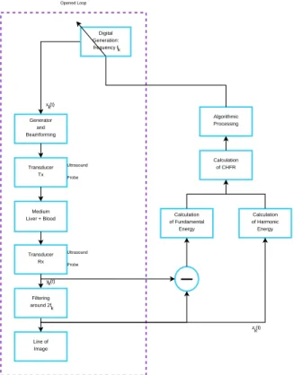
The principle of tissue harmoning imaging including feed-back is described in Fig. 1. At the iteration k, a pulse xk(t) with a frequency fk was transmitted. Its echo yk(t) was fil-tered around 2 fk to form a radiofrequency line of the har-monic image Ik. From the CHFR measured on this image
Ik, a new transmit frequency fk+1was computed by the
algo-rithm to optimize the CHFR on the next image Ik+1.
2.1
Transmitted Signal
The pulse signal xk(t) at transmit frequency fkwas com-puted digitally with Matlab (Mathworks, Natick, MA, USA):
xk(t) = A · wk(t). (2) The sinus modulated by a Gaussian function [3] wk,p(t) was constructed such as:
wk(t) = exp −(t − t0) 2 Nc 2 fk sin(2π fkt), (3)
where t is the time, t0 the time for which the Gaussian
func-tion is maximum, Nc the cycle number. Note that to limit
Generator and Beamforming Transducer Tx Transducer Rx Medium Liver + Blood Line of Image Algorithmic Processing Calculation of CHFR Opened Loop Calculation of Fundamental Energy Calculation of Harmonic Energy z (t)k Filtering around 2f Digital Generation: frequency f Ultrasound Probe Ultrasound Probe y (t)k x (t)k k k
Figure 1: Block diagram of adaptive tissue harmonic imaging.
direct transmission around harmonic frequencies, the trans-ducer bandwidth must be shared between the transmit and receive bandwidths [3]. The cycle number Ncwas set so that the transmit bandwidth was equal to the half-bandwidth of the transducer.
The amplitude of the driving pressure A was then adjusted so that the power of the pulse xk(t) was constant:
A = v t A2 0· Pxref Pw , (4)
where A0 is the driving pressure amplitude of the reference
signal xref. This signal xref was calculated at the transducer centre frequency. Its power Px
ref constituted the reference
power, while Pwwas the power of the signal wk. The power of the transmitted wave thus remained constant by adjusting the amplitude signal A.
2.2
Cost-function
In the receiver, the CHFRkwas computed as the ratio of the harmonic power Ph,kbackscattered and the fundamental power Pf,k: CHFRk=10 · log10 Ph,k Pf,k ! , (5)
The harmonic power was measured from the filtered echo
zk(t) and the fundamental power was measured from the fun-damental echo which was equals to the difference between
yk(t) and zk(t). The harmonic echo zk(t) formed the harmonic image by filtering yk(t) at 2 fkand with a bandwidth equal to the half-bandwidth of the transducer.
The gain GdB was also defined between the optimized system and the non-optimized system. The CHFR obtained
with the non-optimized system was determined at the two-thirds of the transducer centre frequency 2/3 fc [10]. The contrast gain GdB is obtained by the next equation:
GdB = CHFR( f
⋆)
CHFR(2/3 fc). (6)
2.3
Iterative Optimization Algorithm
The algorithm was based on the principle of the gradient descent [13]. It determined a new transmit frequency fk+1
for the next pulse to optimize the CHFRk+1by the following
recurrence relation:
fk+1= fk+ µk· dk, (7)
The first coefficient µkset the speed convergence such as:
µk= 0 if k 6 3; ∆ f if k = 4; µk−1 if sgn(∇CHFR( fk)) = sgn(∇CHFR( fk−1)); µk−1 2 if sgn(∇CHFR( fk)) , sgn(∇CHFR( fk−1)). (8) where ∆ f fixed at 100 kHz provided the best compromise between convergence speed and robustness, sgn(t) the sign function that is equal to 1 if t > 0, 0 if t = 0 and −1 if t < 0, and the CHFR gradient defined by:
∇CHFR( fk) =CHFRk− CHFRk−1
fk− fk−1
. (9)
The second coefficient dkset the direction such as:
dk= 1 if k 6 3; 1 if sgn(∇CHFR( fk)) = sgn(∇CHFR( fk−1)); −1 if sgn(∇CHFR( fk)) , sgn(∇CHFR( fk−1)). (10) In order to compute µk and dk, the system operated in open-loop for the first three iterations (k = {1, 2, 3}). The first three frequencies f1, f2 and f3 were chosen initially.
Their good choice could increase the convergence speed, but it was not decisive to reach the optimal CHFR, when the cost-function was concave.
3
Evaluation of the Method in
Simu-lations
3.1
Simulation Model
The simulation model followed the same process as the experimental setup (Fig. 1).
A pulse signal was generated digitally at iteration k by the equation 2. Note that the pressure levels A0was 400 kPa and
the number cycle Ncwas 4 to restrict the pulse bandwidth at the half-bandwidth of the transducer. However before send-ing this signal to the ultrasound probe, a beamformsend-ing step was added. The linear sweeping [14] enabled to focalized at 15 mm-depth with eight elements of the ultrasound probe. The pulse signal were then filtered by the transfer function of the ultrasound probe; centred at 3.5 MHz with a fractional bandwidth of 63% to −3 dB.
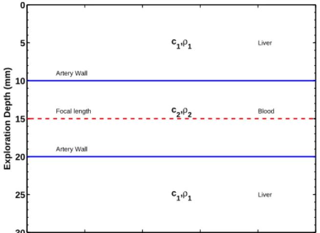
This wave nonlinearly propagated in a liver-mimicking medium where the properties was described in table 1. In
Table 1: Mecanical Properties of the Medium Explored [14]. Liver ρ1 N(1050 kg/m3,30 kg2/m6) c1 N(1578 m/s, 30 : m2/s2) Blood ρ2 N(1060 kg/m3,2.5 kg2/m6) c2 N(1584 : m/s, 2.5 : m2/s2)
this medium, a 10 mm-diameter artery was at 15 mm of the surface. Moreover, the wave propagation was solved by the model developped by Anderson [15].
0 5 10 15 20 25 30 Exploration Depth (mm) Artery Wall Focal length Artery Wall c1,ρ1 c2,ρ2 c1,ρ1 Liver Blood Liver
Figure 2: Grid of Medium Properties: c is the wave celerity and ρ is the density. The ultrasound probe was at the depth
of 0 mm.
Finally, the echoes were measured and filtered by the transfer function of the same ultrasound probe to form a ra-diofrequency line.
3.2
Simulation Results
The empirical optimization was the first simulation pre-sented in Fig. 3 by a dashed line. The results represent the
CHFRas a function of the transmit frequency. The trans-mit frequency was swept by step of 0.125 MHz between 1 and 4 MHz. Firstly, the CHFR had a global maximum. This result showed that the CHFR can be improved by prop-erly choosing the transmit frequency. This property was also interesting, because an automatic search could be achieved more easily by a gradient algorithm. Secondly, the maxi-mum value of the CHFR was −29 dB at 1.625 MHz and the gain GdB was 8.3 dB. This result showed that the best trans-mit frequency was not the two-thirds of the transducer centre frequency. This point confirms again the necessity of opti-mizing the imaging process.
The maximum CHFR was then automatically sought us-ing the gradient algorithm. The Fig. 3 shows the CHFR measured at each iteration k by a solid line. The transmit frequency converged to a stable value after height iterations at 1.6 MHz. Note that the CHFR and the gain GdB obtained automatically were the same than those obtained empirically in the first simulation.
To sum up, the results in Fig. 3 confirm the necessity of optimizing the imaging system. It was possible to find
1 1.25 1.5 1.75 2 2.25 2.5 2.75 3 3.25 3.5 3.75 4 −42 −40 −38 −36 −34 −32 −30 −28 Frequency f (MHz) CTHF (dB) 1 2 3 4 5 6 7 8 10 15 20 2/3 fc G dB = 8.3 dB Empirical Optimization Automatic Optimization
Figure 3: Simulation of the CHFR optimization. The dashed line represents an empirical optimization and the solid line represents an automatic optimization by iterative searching
of the optimal transmit frequency.
automatically the transmit frequency which maximized the
CHFR. No a priori knowledge was required, except for the choice of the first three transmit frequencies which impacted the speed of convergence.
As an illustration, the Fig. 4 represents the image for the two-thirds of the transducer centre frequency and the image for the optimal frequency f⋆ with logarithm compression.
At the top of the images, the liver harmonic response was stronger with the optimal frequency. The contrast between the top (liver) and the middle (blood) was thus increased if the optimal transmit frequency was used.
lateral (mm) depth (mm) 0 2 4 6 8 10 0 5 10 15 20 25 30 −55 −50 −45 −40 −35 −30 −25 (a) 2/3 fc=2.3 MHz lateral (mm) depth (mm) 0 2 4 6 8 10 0 5 10 15 20 25 30 −55 −50 −45 −40 −35 −30 −25 (b) f⋆=1.6 MHz
Figure 4: Synthetic Image where the transmit frequency was the two-thirds of the transducer centre frequency and the
optimal frequency f⋆.
4
Experimental Validation
The aim of this experiment was to confirm experimentally the results obtained in the simulation.
4.1
Experimental Setup
The experimental setup is presented in Fig. 1. The trans-mitted signal xk(t) was first generated digitally using equa-tion 2 by a personal computer. It was sent from an ultra-sound scanner to the medium via an ultraultra-sound probe. This wave insonified the medium. The reception system collected the echoes yk(t) and filtered around 2 fkto form a line of the harmonic image.
4.1.1 Ultrasound Scanner and Transducers
The transmitted signal xk(t) was sent to an “open” ultra-sound scanner (MultiX WM, M2M, Les Ulis, France) via USB. This ultrasound scanner automatically duplicated the signal xk(t) for each element of the ultrasound probe. It ap-plied the delays necessary to obtain phased-array beamform-ing [14]. The signals were then transmitted to a linear ar-ray of 128 elements (Vermon SA, Tours, France), centred at 4 MHz with a fractional bandwidth of 53% to −3 dB. The wave focused on 28 mm from the surface. Note that the pulse was chosen with a cycle number corresponding to 55% of the relative bandwidth at the transducer centre frequency (i.e. Nc =4) and with a pressure level A0of 400 kPa at the
focal point.
4.1.2 Medium Explored
The wave propagated through a tissue-mimicking phan-tom (model 054GS, General Purpose Ultrasound Phanphan-tom, CIRS, Norfolk, VA, USA), including an hyperechoic target at a 4 cm-depth and with a 6 dB-contrast.
4.2
Experimental Results
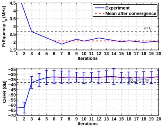
The experimental results presented in Fig. 5 show the transmit frequency and the CHFR during the iterations. The error bars show the standard deviation of the CHFR in the image at the iteration k. The CHFR converged to its optimal value after six iterations for a transmit frequency of 2.1 MHz. The mean CHFR after convergence was around −32.8 dB,
i.e.a mean gain of 5.2 dB.
1 2 3 4 5 6 7 8 9 10 11 12 13 14 15 16 17 18 19 20 1.5 2 2.5 3 3.5 4 4.5 Iterations FrEquency f 0 (MHz) 2/3 f c Experiment
Mean after convergence
1 2 3 4 5 6 7 8 9 10 11 12 13 14 15 16 17 18 19 20 −70 −65 −60 −55 −50 −45 −40 −35 −30 −25 Iterations CHFR (dB) GdB = 5.2 dB
Figure 5: Automatic optimization experiment of CHFR
These results confirmed the experimental feasibility of the method. Note that there was a difference between the gain value in our simulation and that in our experiment. This difference may be explained by the different transducer prop-erties. In simulation, the transducer centre frequency was lower than in experiment to decrease the simulation time.
As an illustration, the Fig. 6 represents the image for the two-thirds of the transducer centre frequency and the im-age for the optimal frequency f⋆ with logarithm
compres-sion. At the middle of the images, the hyperechoic target energy backscattered was increased to 12% with the optimal frequency. Moreover, the power ratio between the hypere-choic target and the surrounding medium was increased to
8%. The contrast was thus increased when the optimal trans-mit frequency was used.
angle (°) depth (cm) −1 −0.8 −0.6 −0.4 −0.2 0 0.2 0.4 0.6 0.8 1 2.5 3 3.5 4 4.5 5 5 10 15 20 25 30 35 40 45 (a) 2/3 fc=2.7 MHz angle (°) depth (cm) −1 −0.8 −0.6 −0.4 −0.2 0 0.2 0.4 0.6 0.8 1 2.5 3 3.5 4 4.5 5 5 10 15 20 25 30 35 40 45 (b) f⋆=1.6 MHz
Figure 6: Experimental Image where the transmit frequency was the two-thirds of the transducer centre frequency and
the optimal frequency f⋆.
5
Discussions and Conclusion
CHFRoptimization in tissue harmonic imaging was per-formed automatically, without taking into account a priori knowledge of the medium or the transducer, except for the first three values of the transmit frequency knowing that their selection had only impact on the convergence speed. The al-gorithm automatically determined an appropriate value for the transmit frequency within only a few iterations. To date, the recommended transmit frequency was the two-thirds of the transducer centre frequency, but this empirical setting cannot enable the optimum performances. The proposed al-gorithm itself adjusted the transmit frequency to maximize the harmonic power backscattered while minimizing the fun-damental power backscattered within the transducer band-width.
Our method was easy to use for two reasons. Optimiza-tion was iteratively achieved by using first an easily imple-mented algorithm and by using second a single parameter. A major advantage of our approach is that it was independent of the medium explored since the cost-function was exclusively based on the input and the output measurements of our sys-tem. An interesting consequence is that our method can be applied to any imaging system.
Note that a real-time implementation was possible, since the computation time was insignificant. However, the method required a programmable analogue transmitter. Moreover, although our technique could offer an optimal frequency for each line of the image, it was preferable to perform optimiza-tion on the whole image. The image can be consistent with a single resolution.
To conclude, the method described ensured optimal CHFR by adaptively selecting the transmit frequency. Through our new approach, manufacturers and clinicians do not need to set themselves the transmit frequency.
Our closed-loop method can be adapted using a larger number of techniques for tissue harmonic imaging. The only difficulty remaining is in the instrumentation. However the development of new imaging methods based on chirp or time reversal are also needed for such instrumentation.
References
[1] P. J. A. Frinking, A. Bouakaz, J. Kirkhorn, F. J. Ten Cate, and N. de Jong. Ultrasound contrast imag-ing, Current and new potential methods. Ultrasound
Med. Biol. 26(6), 965–975 (2000).
[2] F. Tranquart, N. Grenier, V. Eder, and L. Pourcelot. Clinical Use of Ultrasound Tissue Harmonic Imaging.
Ultrasound Med. Biol., 25(6), 889–894 (1999). [3] M. A. Averkiou. Tissue Harmonic Imaging. In Proc.
IEEE Ultrason. Symp. 2, 1563–1572 (2000).
[4] Qingyu Ma, Xiufen Gong, and Dong Zhang. Third Order Harmonic Imaging for Biological Tissues using Three Phase-Coded Pulses. Ultrasonics
44(Supplement), e61–e65 (2006).
[5] D. H. Simpson, C. T. Chin, and P. N. Burns. Pulse In-version Doppler: A New Method for Detecting Nonlin-ear Echoes from Microbubble Contrast Agents. IEEE
Trans. Ultrason., Ferroelectr., Freq. Control 46(2), 372–382 (1999).
[6] Q. Ma, Y. Ma, X. Gong, and Dong Zhang. Improve-ment of Tissue Harmonic Imaging using the Pulse-Inversion Technique. Ultrasound Med. Biol. 31(7), 889–894 (2005).
[7] G. A. Brock-fisher, M. D. Poland, and P. G. Rafter. Means for Increasing Sensitivity in Non-linear Ultra-sound Imaging Systems, US Patent 5577505 (1996). [8] J. Song, S. Kim, H. Sohn, T. Song, and Yang Mo
Yoo. Coded Excitation for Ultrasound Tissue Harmonic Imaging. Ultrasonics 50(6), 613–619 (2010).
[9] J. Song, J. H. Chang, T. Song, and Y. Yoo. Coded Tis-sue Harmonic Imaging with Nonlinear Chirp Signals.
Ultrasonics 51(4), 516–521 (2011).
[10] J. A. Hossack, P. Mauchamp, and L. Ratsimandresy. A High Bandwidth Transducer Optimized for Harmonic Imaging. In Proc. IEEE Ultrason. Symp. 2, 1021–1024 (2000).
[11] S. M´enigot, A. Novell, I. Voicu, A. Bouakaz, and J.-M. Girault. Adaptive contrast imaging: Transmit fre-quency optimization. Physics Procedia 3(1), 667–676 (2010).
[12] S. M´enigot. Commande optimale appliqu´ee aux syst`emes d’imagerie ultrasonore. PhD thesis, Univer-sit´e Franc¸ois-Rabelais de Tours, Tours, France (2011). [13] B. Widrow and S. Stearns. Adaptive Signal Processing.
Prentice Hall, Englewood Cliffs, USA (1985).
[14] Thomas Szabo. Diagnostic Ultrasound Imaging: Inside
Out. Academic Press, London, UK (2004).
[15] M. E. Anderson. A 2D Nonlinear Wave Propagation Solver Written in Open-Source MATLAB Code. In