HAL Id: cea-01541913
https://hal-cea.archives-ouvertes.fr/cea-01541913
Submitted on 19 Jun 2017
HAL is a multi-disciplinary open access
archive for the deposit and dissemination of
sci-entific research documents, whether they are
pub-lished or not. The documents may come from
teaching and research institutions in France or
abroad, or from public or private research centers.
L’archive ouverte pluridisciplinaire HAL, est
destinée au dépôt et à la diffusion de documents
scientifiques de niveau recherche, publiés ou non,
émanant des établissements d’enseignement et de
recherche français ou étrangers, des laboratoires
publics ou privés.
seen by BRITE -Constellation ⋆ : Pulsation, differential
rotation, and angular momentum transfer
T. Kallinger, W. Weiss, P. Beck, A. Pigulski, R. Kuschnig, A. Tkachenko, Y.
Pakhomov, T. Ryabchikova, T. Lüftinger, P.L. Palle, et al.
To cite this version:
T. Kallinger, W. Weiss, P. Beck, A. Pigulski, R. Kuschnig, et al.. Triple system HD 201433 with
a SPB star component seen by BRITE -Constellation ⋆ : Pulsation, differential rotation, and
angu-lar momentum transfer. Astronomy and Astrophysics - A&A, EDP Sciences, 2017,
�10.1051/0004-6361/201730625�. �cea-01541913�
arXiv:1704.01151v1 [astro-ph.SR] 4 Apr 2017
April 6, 2017
Triple system HD 201433 with a SPB star component seen by
BRITE - Constellation
⋆
: Pulsation, differential rotation, and angular
momentum transfer
T. Kallinger
1, W. W. Weiss
1, P. G. Beck
2, 3, 4, A. Pigulski
5, R. Kuschnig
1, 6, A. Tkachenko
7, Y. Pakhomov
8, T.
Ryabchikova
8, T. Lüftinger
1, P. L. Palle,
3, 4, E. Semenko
9, G. Handler
10, O. Koudelka
6, J. M. Matthews
11, A. F. J.
Moffat
12, H. Pablo
12, A. Popowicz
13, S. Rucinski
14, G. A. Wade
15, and K. Zwintz
161 Institute for Astrophysics, University of Vienna, Türkenschanzstrasse 17, 1180 Vienna, Austria
2 Laboratoire AIM, CEA/DRF CNRS - Université Denis Diderot IRFU/SAp, 91191 Gif-sur-Yvette Cedex, France 3 Instituto de Astrofísica de Canarias, E-38200 La Laguna, Tenerife, Spain
4 Departamento de Astrofísica, Universidad de La Laguna, E-38206 La Laguna, Tenerife, Spain 5 Instytut Astronomiczny, Uniwersytet Wrocławski, Kopernika 11, 51-622 Wrocław, Poland
6 Institut für Kommunnikationsnetze und Satellitenkommunikation, Technical University Graz, Inffeldgasse 12, 8010 Graz, Austria 7 Instituut voor Sterrenkunde, K.U. Leuven, Celestijnenlaan 200D, 3001 Leuven, Belgium
8 Institute of Astronomy, Russian Academy of Sciences, Pyatnitskaya 48, 119017 Moscow, Russia 9 Special Astrophysical Observatory, Russian Academy of Sciences, 369167, Nizhnii Arkhyz, Russia 10 Nicolaus Copernicus Astronomical Center, ul. Bartycka 18, 00-716 Warsaw, Poland
11 Department of Physics and Astronomy, University of British Columbia, Vancouver, BC V6T1Z1, Canada
12 Département de physique and Centre de Recherche en Astrophysique du Québec (CRAQ), Université de Montréal, CP 6128, Succ. Centre-Ville, Montréal, Québec, H3C 3J7, Canada
13 Institute of Automatic Control, Silesian University of Technology, Akademicka 16, 44-100 Gliwice, Poland
14 Department of Astronomy & Astrophysics, University of Toronto, 50 St. George Street, Toronto, Ontario, M5S 3H4, Canada 15 Department of Physics, Royal Military College of Canada, PO Box 17000, Station Forces, Kingston, Ontario, K7K 7B4, Canada 16 Institut für Astro- und Teilchenphysik, Universität Innsbruck, Technikerstrasse 25/8, 6020 Innsbruck, Austria
Received 15 February 2017 / Accepted 28 March 2017
ABSTRACT
Context.Stellar rotation affects the transport of chemical elements and angular momentum and is therefore a key process during
stellar evolution, which is still not fully understood. This is especially true for massive OB-type stars, which are important for the chemical enrichment of the universe. It is therefore important to constrain the physical parameters and internal angular momentum distribution of massive OB-type stars to calibrate stellar structure and evolution models. Stellar internal rotation can be probed through asteroseismic studies of rotationally split non radial oscillations but such results are still quite rare, especially for stars more massive than the Sun. The slowly pulsating B9V star HD 201433 is known to be part of a single-lined spectroscopic triple system, with two low-mass companions orbiting with periods of about 3.3 and 154 days.
Aims.Our goal is to measure the internal rotation profile of HD 201433 and investigate the tidal interaction with the close companion.
Methods. We used probabilistic methods to analyse the BRITE - Constellation photometry and radial velocity measurements, to
identify a representative stellar model, and to determine the internal rotation profile of the star.
Results.Our results are based on photometric observations made by BRITE - Constellation and the Solar Mass Ejection Imager on
board the Coriolis satellite, high-resolution spectroscopy, and more than 96 years of radial velocity measurements. We identify a sequence of nine frequency doublets in the photometric time series, consistent with rotationally split dipole modes with a period spacing of about 5030 s. We establish that HD 201433 is in principle a solid-body rotator with a very slow rotation period of 297±76 days. Tidal interaction with the inner companion has, however, significantly accelerated the spin of the surface layers by a factor of approximately one hundred. The angular momentum transfer onto the surface of HD 201433 is also reflected by the statistically significant decrease of the orbital period of about 0.9 s during the last 96 years.
Conclusions. Combining the asteroseismic inferences with the spectroscopic measurements and the orbital analysis of the inner
binary system, we conclude that tidal interactions between the central SPB star and its inner companion have almost circularised the orbit. They have, however, not yet aligned all spins of the system and have just begun to synchronise rotation.
Key words. asteroseismology - stars: individual: HD 201433 - stars: oscillations - stars: interior - stars: rotation - stars: binaries:
general
Send offprint requests to: [email protected]
⋆ Based on data collected by the BRITE - Constellation satellite mis-sion, built, launched and operated thanks to support from the Austrian Aeronautics and Space Agency and the University of Vienna, the
Cana-dian Space Agency (CSA), and the Foundation for Polish Science & Technology (FNiTP MNiSW) and National Science Centre (NCN), the Hermes spectrograph mounted on the 1.2 m Mercator Telescope at the Spanish Observatorio del Roque de los Muchachos of the Instituto de
1. Introduction
Massive stars are important for the chemical enrichment of the universe. Slowly pulsating B (SPB) stars are not amongst the most massive stars, but they share a similar internal structure and are therefore ideal to improve our understanding of massive stars.
Slowly pulsating B stars (SPB) were introduced to the zoo of variable stars by Waelkens (1991). They are non-radial multi-periodic oscillators on the main sequence between spectral type B3 and B9, with an effective temperature ranging from about
11,000 to 22,000 K, and a mass between 2.5 and 8 M⊙ (e.g.
Aerts et al. 2010). They oscillate in high-order gravity (g) modes
with frequencies typically ranging from 0.5 to 2 d−1, which are
driven by the κ-mechanism acting due to the iron-group element opacity bump (e.g. Dziembowski et al. 1993). Consecutive ra-dial order n gravity modes of the same spherical degree l are ex-pected to be equally spaced in period, and deviations from this regular pattern carry information about physical processes in the near-core region (e.g. Miglio et al. 2008).
SPB stars are expected to be dominated by a convective core and a radiative envelope, and therefore experience internal mix-ing processes, which have a significant influence on the lifetime of the star by enhancing the size of the convective region in which mixing of chemical elements occurs. Such a mixing might be induced by convective core overshooting but also by internal differential rotation (e.g. Aerts et al. 2003; Dupret et al. 2004). Despite their importance for realistic stellar structure and evo-lution models of massive stars, the physical details describing these processes are hardly known. This is mainly because of the small number of detailed investigations of SPB stars, partly due to the few identified modes in these studies (for a recent review see Aerts 2015).
The Canadian space telescope MOST (Walker et al. 2003; Matthews et al. 2004) was very successful in providing the high quality data of SPB stars that are necessary to challenge theory (e.g. Walker et al. 2005; Aerts et al. 2006; Gruber et al. 2012; Jerzykiewicz et al. 2013). The breakthrough in observing SPB stars came, however, with the Kepler mission. Only recently, Pápics et al. (2014, 2015) reported on the detection of a rotation-ally affected series of g-modes in the two SPB stars KIC 7760680 and KIC 10526294 that show clear signatures of chemical mix-ing and rotation and which enabled the first actual seismic mod-elling of SPB stars. A limitation in this respect is that Kepler can only observe fairly faint stars, for which additional observational constraints (e.g., from high resolution spectroscopy or interfer-ometry) are difficult to obtain.
HD 201433 (HR 8094, V389 Cyg) is one of the brightest stars (V≃5.61 mag) suspected to be a SPB star (due to its position in the Hertzsprung-Russel diagram). The B9V star is known to be member of a single-line spectroscopic triple system (Barlow
1989). The most recent determinations of Teff =12193±360 K,
log g = 4.24±0.2, and v sin i = 15 km/s were published by Takeda et al. (2014). Its Hipparcos parallax is 8.64 ± 0.55 mas (van Leeuwen 2007), from which we obtain an absolute visual
magnitude of MV =0.29 ± 0.14 mag. Interpolation in the tables
of Lejeune & Schaerer (2001) for [Fe/H] = 0.0 (see Sec. 9.3)
in-dicates a bolometric correction of BCV = −0.70 ± 0.05. With
Mbol,⊙ =4.76 mag (Kopp & Lean 2011) we then obtain L/L⊙=
Astrofísica de Canarias, and the Solar Mass Ejection Imager, which is a joint project of the University of California San Diego, Boston Col-lege, the University of Birmingham (UK), and the Air Force Research Laboratory.
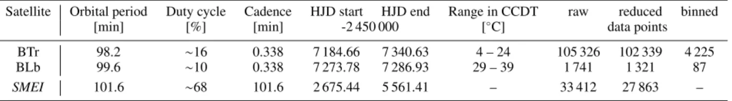
Fig. 1.Point spread function (PSF) positions for the BTr observations (during observing setup 3) in the CCD subraster. The red ellipses in-dicate the limit outside of which data points are eliminated for further analysis (light grey points). We note that even though the ellipse on the left hand side appreas to be misaligned it correctly reflects the distribu-tion of the PSF posidistribu-tions.
115 ± 15. These parameters locate HD 201433 close to the cool border of the SPB domain.
In this paper we report high-precision photometric
observa-tions of HD 201433 with BRITE - Constellation1, which is an
ar-ray of five nanosatellites devoted to high-precision, long-term photometry of bright stars as is described by Weiss et al. (2014). Our photometric analysis is primarily based on 156 days of BRITE-Toronto (BTr) observations supplemented by about 13 days of BRITE-Lem (BLb) data (see Tab. 1). The data prod-ucts and necessary post-processing are described in Sec. 2 & 3. The Bayesian frequency analysis (Sec. 4) reveals a sequence of nine significant close pairs of frequencies, consistent with ro-tationally split dipole modes, from which we extracted an av-erage period spacing and rotational splittings (Sec. 5). In Sec. 6 we demonstrate that our interpretation of the BRITE photome-try is fully consistent with the signal found in the almost eight-year long SMEI observations. We then construct a dense stellar model grid and search for a representative model of HD 201433 (Sec. 7), which we use in Sec. 8 to infer the internal rotation pro-file. To complement the space photometry we obtain new high-resolution spectra which extend the time base to slightly more than 96 years with a total of 231 spectra usable for an orbital analysis. Based on an entirely Bayesian analysis of the radial ve-locity measurements we improve the published orbital elements and find evidence for a continuously decreasing orbital period. Putting this in context of our asteroseismic and spectroscopic results we conclude that the main component of HD 201433 is a SPB star of about three solar masses showing no significant rota-tional gradient throughout most of its interior. However, we find indications for tidal interaction with a close companion, causing an acceleration of the outermost envelope. We discuss our find-ings for HD 201433 in a broader astrophysical context in Sec. 10 and summarise our analysis in Sec. 11.
2. BRITE photometry of HD 201433
The photometric observations used in this study were carried out with two of the five BRITE - Constellation satellites. Each
Table 1.Overview of the photometric observations of HD 201433 obtained with BRITE-Toronto2, BRITE-Lem3, and the Coriolis/SMEI satellite. The last three columns give the number of data points of the raw, reduced, and subsequently binned data set.
Satellite Orbital period Duty cycle Cadence HJD start HJD end Range in CCDT raw reduced binned [min] [%] [min] -2 450 000 [◦C] data points BTr 98.2 ∼16 0.338 7 184.66 7 340.63 4 – 24 105 326 102 339 4 225 BLb 99.6 ∼10 0.338 7 273.78 7 286.93 29 – 39 1 741 1 321 87 SMEI 101.6 ∼68 101.6 2 675.44 5 561.41 – 33 412 27 863 –
of the 20×20×20 cm satellites hosts an optical telescope of 3 cm aperture, feeding an uncooled CCD, and is equipped with a sin-gle filter. Three nanosats have a red filter (550–700 nm) and two have a blue filter (390–460nm). The orbital periods are close to 100 min, enabling continuous observations of the chosen target fields for about 5–30 min per orbit.
The detector is a Kodak KAI-11002M CCD with about 11
million 9 × 9 µm pixels (plate scale of 27.3′′ per pixel), a
14-bit A/D converter, an inverse gain of about 3.5 e−/ADU, and a
readout noise and dark current of about 16 e− and 20 e−/s per
pixel, respectively, at +20◦C. The saturation limit of the pixels
at this temperature is about 13 000 ADU, with the response being linear up to about 9 000 ADU. Further details about the detector and data acquisition of BRITE - Constellation are described by Pablo et al. (2016)
A problem affecting the BRITE nanosatellites is the higher-than-expected sensitivity of the CCDs to particle radiation, which posed a major threat to the lifetime and effectiveness of the BRITE mission. The impact of high-energy protons causes the emergence of hot and warm pixels at a rate much higher than originally expected. The affected pixels more easily gen-erate thermal electrons and thereby significantly impair the pho-tometric precision of the observations. An additional important problem that appeared after several months of operation was the charge transfer inefficiency also caused by the protons. There were serious problems in the early phase of the mission, but thanks to slowing the readout time and adopting a chopping tech-nique for data acquisition, the effect of CCD radiation damage on the photometry is now significantly reduced (Popowicz et al. 2017).
Satellite pointing is adjusted slightly between consecutive exposures in the chopping mode, so that the target PSFs alter-nate between two positions (about 20 pixels apart) on the CCD. This means that the PSF-free part of a given subraster image acts as a dark image for the subsequent exposure and subtracting con-secutive exposures results in an image with one negative and one positive target PSF. The background defects are thereby almost entirely removed. More details about this technique are given by Popowicz et al. (2017).
HD 201433 was one of the targets in the BRITE -Constellation Cygnus II field and was observed with
BRITE-Toronto2for about 156 days in June–November 2015 typically
48 times per BRITE orbit with an average cadence of 5 s ex-posures every 20.3 s. A significantly shorter data set was
ob-tained with BRITE-Lem3, which observed HD 201433 for about
13 days in September 2015 for typically 30 times per orbit (see Tab. 1).
2 The Canadian satellite BRITE-Toronto was launched on June 19, 2014, into a slightly elliptical and almost Sun-synchronous orbit and is equipped with a red filter.
3 The Polish BRITE-Lem was launched on September 21, 2013, into an elliptical orbit and is equipped with a blue filter.
Fig. 2.Correlations between HD 201433 flux measurements and BTr housekeeping parameters (CCD temperature and the X and Y positions of the PSF) as obtained during observing setup 3. The left and right panels correspond to flux measurements extracted from the “left” and “right” part of the subraster image (see Fig. 1). The bottom panels show the residual time series phased with the satellite’s orbital period. Red lines indicate linear (top panel) and polynomial (middle panels) fits and a boxcar filter (bottom panel).
As the stellar flux is extracted from differential images (chopping mode) no bias, dark, and background corrections are necessary. The remaining main step is to identify the op-timal apertures and to extract the flux within these apertures (Popowicz et al. 2017). The light curves resulting from this pipeline reduction are deposited in the BRITE - Constellation data archive from where we extracted the data of HD 201433 and applied some post-processing routines, as are described in the following.
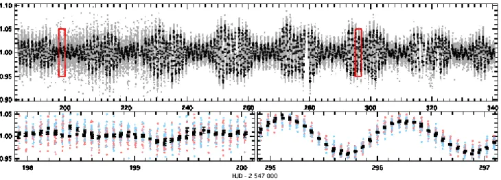
Fig. 3.Final light curve of HD 201433 as obtained with BTr. The grey and black dots in the top panel represent the full and binned data, respectively. The bottom panels show enlargements of the full data set (red boxes in the top panel) with the red and blue symbols indicating flux measurements extracted from the “left” and “right” part of the subraster frame (see Fig. 1). Black filled circles correspond to data binned into two bins per orbit.
3. BRITE data post-processing
The raw stellar flux still includes instrumental effects and obvi-ous outliers and therefore needs some post-processing. The BTr
data came in two different setups4and five data blocks of
approx-imately equal length, which we treated independently. The first setup at the beginning of the observing run addressed 24 stars in the field but had to be reduced to 18 stars (2nd setup), because of data transfer limitations. Subdivision of the dataset into blocks was required due to a limit of typically 30 000 frames for the standard data reduction software.
Adapting the recipe of Pigulski et al. (2016) we perform the following steps for each of the five blocks:
– Divide the data set into two sets corresponding to the
alter-nating PSF position on the CCD subraster. (see Fig. 1).
– Compute a 2D histogram of the X/Y positions and fit a 3D
multivariate Gaussian to it. Measurements that were obtained with the PSF centre positioned outside three times the widths of the Gaussian (see Fig. 1) are eliminated from further pro-cessing. This procedure identifies most of the outliers (about 2.5% of the original data) and rejects them.
– The procedure resumes with the “cleaned" data set and
ap-plies a 4σ-clipping to the whole data set, where σ was de-termined from the complete set. The procedure results in the elimination of additional ∼0.3% of all data points.
– To better access the instrumental correlations we first
pre-whiten the two highest amplitude frequencies (see Sec. 4), which are subsequently added back after post-processing of the data.
– In the case of HD 201433 the instrumental flux increases
typ-ically by 5 – 7 ADU/s per◦C with increasing CCD
temper-ature. A quadratic fit with the CCD temperature is sufficient to correct for this temperature correlation (see top panel of Fig. 2).
– Pixel-to-pixel sensitivity variations of the detector are
re-flected in correlations between the instrumental flux and the
4 Setup refers here to a set of camera parameters but also to subraster positions on the CCD. Setups may change at the begining of a run (dur-ing optimis(dur-ing of the observations) or due to add(dur-ing/remov(dur-ing a star during the run, where for each parameter change a whole new setup is generated with unique ID.
PSF position on the CCD (about 3 – 5 ADU/s per pixel). We correct for this with polynomial fits (middle panels of Fig. 2).
– Residual instrumental signal is apparent when phasing the
instrumental flux with the satellite’s orbital period. We cor-rect for the high-overtone signal with a 200 point box-car filter in the phase plot (bottom panels of Fig. 2).
– The residual instrumental flux is then divided by its average
value for conversion to relative flux.
The ten reduced data sets (two for each setup) are then sim-ply stitched together, where no significant offsets at the subset interfaces are found. The final light curve of HD 201433 con-sists of about 102 000 individual measurements and is shown in Fig. 3. The post-processing reduces the point-to-point scatter of the BTr data of HD 201433 from about 46 to 34 ADU/s (or ∼0.9%).
The intrinsic variability of HD 201433 acts on time scales of no shorter than a few hours; hence, the average cadence of about
20.3 s (which corresponds to a Nyquist frequency of ∼2130 d−1)
is unnecessarily short. Given this and because the frequency analysis (see Sec. 4) requires good estimates for the uncertainties of the individual measurements we bin the light curve. To keep the dominant cadence short enough (i.e., the Nyquist frequency high enough) we bin the typically 48 measurements per BRITE orbit into two bins, where the standard deviation of the origi-nal measurements within a given bin provides a good estimate for the photometric accuracy. The binned light curve consists of about 4 200 data points with a median cadence of ∼8.13 min ( fnyq ≃89 d−1) and an average error of about 2.1 ppt.
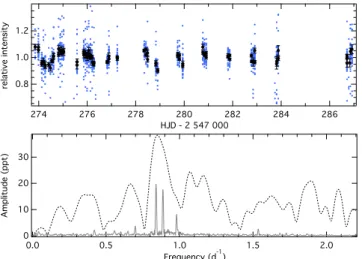
The BLb raw dataset of HD 201433 has a considerably shorter time base than the BTr observations and is due to the higher CCD temperature also much noisier. The original ∼1 700 measurements reduce to about 1 300 useful data points in the post-processed light curve (see Fig. 4). Binning of the typically 30 measurements per BRITE orbit results in 87 data points with a median cadence of ∼5.4 min and an average error of about 16 ppt.
4. Frequency analysis
SPB stars are expected to show long-period g modes in a fre-quency range of up to a few cycles per day. This is well
sepa-30 20 10 0 Amplitude (ppt) 2.0 1.5 1.0 0.5 0.0 Frequency (d-1) 1.2 1.0 0.8 relative intensity 286 284 282 280 278 276 274 HJD - 2 547 000
Fig. 4.Final light curve (top) of HD 201433 as obtained by BLb, with black and blue symbols corresponding to the binned and unbinned ver-sion, respectively. The bottom panel show the Fourier amplitude spectra of the binned BLb (black dashed line) and BTr (grey line) light curves.
rated from residual instrumental signal and alias peaks due to the
orbital frequency of BTr of ∼14.7 d−1(and multiples of it). We
compute the Fourier amplitude spectrum of the unbinned light
curve and find no significant peak between 2 d−1and the Nyquist
frequency which cannot be attributed to the satellite’s orbital fre-quency. The pulsation spectrum (see Fig. 5) of HD 201433 shows
the strongest peaks between about 0.5 – 1 d−1, and another group
of peaks between about 1.5 – 2 d−1. Above that no significant
power can be found.
An unusual feature in the Fourier spectrum of HD 201433 is that some peaks appear slightly broader than expected from the spectral window function (see insert in Fig. 5). This indi-cates the presence of close frequencies that are separated by less than (or close to) the formal frequency (Rayleigh-) resolution
of 1/T ≃ 0.0064 d−1. Such features are problematic for a
stan-dard frequency analysis (based on a strict pre-whitening proce-dure) because assuming a mono-periodic signal in the vicinity of the considered Fourier peak yields a frequency that corresponds to the weighted average of the intrinsic frequency multiplet and pre-whitening this “wrong” signal causes artificial peaks in the spectrum. Furthermore, it is difficult (or often impossible) to ob-jectively rate the significance of the result and its uncertainties.
We use a probabilistic approach to tackle this problem. Kallinger & Weiss (2016) have developed a fully automated Bayesian algorithm that searches for close frequencies in time series data and tests their statistical significance by comparison to a fit with constant (i.e., no periodic) signal and a fit with a mono-periodic signal. The procedure performs the following steps:
– Compute the Fourier amplitude spectrum up to 2 d−1and
de-termine the frequency with the highest amplitude.
– Fit N functions, F(t,n) =Pn
i=1Aisin [2π( fit + Φi)] + c, to the
time series, where n incrementally increases from 1 to N so that, in total, N models with 1, 2, ..., N sinusoidal compo-nents are fit to the data. A, f , and Φ are the amplitude, fre-quency, and phase of the ith component, respectively. The
parameter c serves as an offset to ensure that R
TF(t)dt =0
even if the duration T of the time series is not an integer multiple of the signal period. For the fit we use a Bayesian
20 15 10 5 0 0.01 0.1 1 -20 0 20 6 4 2 0 1.5 1.0 0.5 0.0 0.4 0.2 0.0 2.0 1.5 1.0 0.5 0.0 Frequency (d-1) Amplitude (ppt) SPW data data - f1 .. f4 data - f1 .. f10 residuals 20 10 0 0.85 0.84 0.83
Fig. 5.Fourier amplitude spectrum of the binned BTr light curve of HD 201433. The two middle panels show the amplitude spectrum af-ter pre-withening of the given frequencies. The bottom panel gives the residual amplitude spectrum after pre-withening with all significant fre-quenices. The right insert in the top panel shows the spectral window function of the BTr dataset. The left insert gives the original spectrum (black line) and the spectral window (red dashed line) centered on the main peak. The green and blue peaks indicate the posterior parameter distributions (arbitralily scaled in amplitude for better visibility) of a single and multiple sine fit with MultiNest, respectively.
nested sampling algorithm (MultiNest; Feroz et al. 2009), and allow the individual frequencies to vary around the ini-tial frequency by ±2/T , and the amplitudes between 0 and 50 times the initial amplitude from the amplitude spectrum. Phases have no initial constraints and can vary from 0 to 1.
– To rate if a signal is statistically significant (i.e., not due to
noise) and if so, which model best represents the data, we
compute the model probability (pn) by comparing the global
evidences5 (z
n) of the fits to those of a fit with a constant
factor (zc). If p = P zn/(zc+P zn) > 0.95 we consider the
solution as real6 and not to be due to noise. If so, the
best-fit model is then the model with pn = zn/P zn >0.95. This
means that in order to be accepted, a multiperiodic solution needs to fit the data considerably better than the monochro-matic solution. Our approach for the statistical significance of a signal compares well to classical approaches like a SNR
>4 (e.g. Breger et al. 1993; Kuschnig et al. 1997) but has the
advantage of providing an actual statistical statement that is based only on the data and that allows us to discriminate be-tween mono- and multi-periodic solutions for closely sepa-rated frequencies. In the present case we tested models with
5 The global evidence is a normalised logarithmic probability delivered by MultiNest describing how good the model fits the data with respect to the uncertainties, parameter ranges, and the complexity of the model. 6 In probability theory an odds ratio of 10:1 (i.e., p=0.9) is considered already as strong evidence (Jeffreys 1998).
up to three components but find that for none of the identified multiplets is a solution with N = 3 statistically significant.
– The best-fit parameters and their 1σ uncertainties are then
computed from the marginalised posterior distribution func-tions as delivered by MultiNest.
– The best-fit model is subtracted from the time series and the
procedure starts from the beginning.
We stop the procedure when p drops below 0.66 (correspond-ing to weak evidence) but we accept only those frequencies with
p > 0.95. We note that the frequency, amplitude, and phase
uncertainties that are computed from the posterior probability distributions compare well with uncertainties determined from other criteria (e.g. Kallinger et al. 2008).
Based on extensive tests with synthetic data (with the sam-pling and noise characteristics of the BTr data of HD 201433) Kallinger & Weiss (2016) have shown that the algorithm is capa-ble to reliably (>99.9%) distinguish between a single frequency and a pair of close frequencies if the frequencies are separated by more than ∼ 0.5/T and their amplitudes are larger than about 1 ppt. The uncertainties of the individual frequencies are thereby only slightly larger than for an unperturbed mono-periodic signal but rarely exceed 0.1/T .
4.1. Frequencies and frequency combinations in the BTr data Our Bayesian frequency analysis algorithm identified 9 “fea-tures” in the binned BTr data of HD 201433 that consist of statis-tically significant closely separated frequencies in addition to a further 11 single frequencies. An example for a pair of close fre-quencies is illustrated in the left insert in Fig. 5, where we show the posterior parameter distributions of the one-frequency and two-frequency model fits for the highest-amplitude peak in the BTr spectrum of HD 201433. The evidence of the two-frequency model is orders of magnitude better than for the one-frequency model (despite the Bayesian “penalty” for introducing additional free model parameters), which indicates – based on solid statis-tical grounds – that more than one frequency is needed to repro-duce the data in this frequency range.
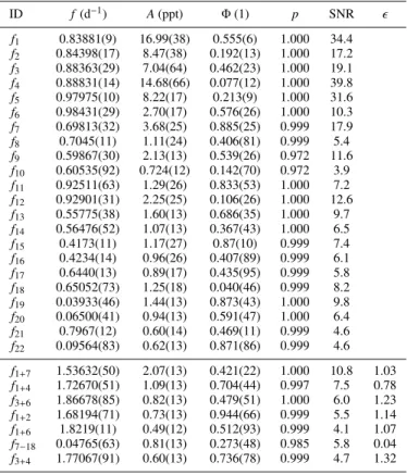
The 29 significant frequencies detected in the BTr data set are listed in Tab. 2. After pre-whitening them from the data, the residual spectrum (see Fig. 5) has an average amplitude of about
110 ppm. The “bump” around 1 d−1, however, indicates that there
is still some undetected signal left (which can well be of in-strumental origin). We searched for linear combinations among all significant frequencies. Out of the 29 detected frequencies we find 22 independent frequencies. The remaining peaks cor-respond to first-order linear combination frequencies (where fi = fj± fk). In order to be identified as a linear combination a
frequency has to fulfil the criterion ( fi−fj∓fk)2< σ2f i+ σ
2 fj+ σ
2 fk
and its amplitude must be smaller than the amplitudes of its
par-ent frequencies ( fj and fk). We also searched for higher-order
combinations but found none. A schematic view of the indepen-dent and combination frequencies is shown in Fig. 6 indicating
that all peaks above 1 d−1 are actually combination frequencies
and that 18 of the 19 peaks between 0.4 and 1 d−1 are part of a
pair of close frequencies fully consistent with rotationally split dipole modes.
4.2. Frequencies in the BLb data
The BLb data set has a much shorter time base and is noisier than the BTr dataset. Consequently, the frequency analysis is more
Table 2.Significant frequencies in the BTr observations of HD 201433. Uncertainties for the frequency f , amplitude A, and phase Φ are given in parentheses in units of the last digit. The phase is defined for the be-ginning of the data set (mHJD = 184.6694) The frequencies listed in the bottom part are combination frequencies, where ǫ gives the devia-tion between the observed frequency and the combinadevia-tion of its parental frequencies in units of the uncertainties (e.g., ǫ < 1 means a difference within 1σ of the formal uncertainties).
ID f(d−1) A(ppt) Φ(1) p SNR ǫ f1 0.83881(9) 16.99(38) 0.555(6) 1.000 34.4 f2 0.84398(17) 8.47(38) 0.192(13) 1.000 17.2 f3 0.88363(29) 7.04(64) 0.462(23) 1.000 19.1 f4 0.88831(14) 14.68(66) 0.077(12) 1.000 39.8 f5 0.97975(10) 8.22(17) 0.213(9) 1.000 31.6 f6 0.98431(29) 2.70(17) 0.576(26) 1.000 10.3 f7 0.69813(32) 3.68(25) 0.885(25) 0.999 17.9 f8 0.7045(11) 1.11(24) 0.406(81) 0.999 5.4 f9 0.59867(30) 2.13(13) 0.539(26) 0.972 11.6 f10 0.60535(92) 0.724(12) 0.142(70) 0.972 3.9 f11 0.92511(63) 1.29(26) 0.833(53) 1.000 7.2 f12 0.92901(31) 2.25(25) 0.106(26) 1.000 12.6 f13 0.55775(38) 1.60(13) 0.686(35) 1.000 9.7 f14 0.56476(52) 1.07(13) 0.367(43) 1.000 6.5 f15 0.4173(11) 1.17(27) 0.87(10) 0.999 7.4 f16 0.4234(14) 0.96(26) 0.407(89) 0.999 6.1 f17 0.6440(13) 0.89(17) 0.435(95) 0.999 5.8 f18 0.65052(73) 1.25(18) 0.040(46) 0.999 8.2 f19 0.03933(46) 1.44(13) 0.873(43) 1.000 9.8 f20 0.06500(41) 0.94(13) 0.591(47) 1.000 6.4 f21 0.7967(12) 0.60(14) 0.469(11) 0.999 4.6 f22 0.09564(83) 0.62(13) 0.871(86) 0.999 4.6 f1+7 1.53632(50) 2.07(13) 0.421(22) 1.000 10.8 1.03 f1+4 1.72670(51) 1.09(13) 0.704(44) 0.997 7.5 0.78 f3+6 1.86678(85) 0.82(13) 0.479(51) 1.000 6.0 1.23 f1+2 1.68194(71) 0.73(13) 0.944(66) 0.999 5.5 1.14 f1+6 1.8219(11) 0.49(12) 0.512(93) 0.999 4.1 1.07 f7−18 0.04765(63) 0.81(13) 0.273(48) 0.985 5.8 0.04 f3+4 1.77067(91) 0.60(13) 0.736(78) 0.999 4.7 1.32
challenging (see the amplitude spectrum in Fig. 4). An indepen-dent analysis gives only one significant peak with a frequency of
0.852±0.003 d−1, which represents a weighted average of f
1and
f4of the formally unresolved frequencies in BLb. We can,
how-ever, fix the frequency to the values determined for the BTr data and fit only the amplitude and phase. We tried various combina-tions of the three largest amplitude frequencies in the BTr data ( f1, f4, f5, f1∧f4, f1∧f5, f4∧f5, and f1∧f4∧f5) and find that
a fit with f1 and f4 gives the (by far) the best model evidence.
The resulting amplitudes and phases are given in Tab. 3. The two frequencies have very similar amplitude ratios and phase differ-ences in the two BRITE passbands, indicating that they have the same spherical degree (e.g. Daszy´nska-Daszkiewicz 2008).
Table 3.Amplitude and phases of f1and f4in the BTr and BLb pass-bands and the corresponding amplitude ratios and phase differences.
ID BTr BLb
A(ppt) Φ(1) A(ppt) Φ(1) Ab/Ar Φb− Φr
f1 16.99(38) 0.555(6) 30.2(3) 0.579(14) 1.78(4) 0.02(2)
3.0 2.5 2.0 1.5 1.0 0.5 0.0 Amplitude (ppt) 1.0 0.9 0.8 0.7 0.6 0.5 0.4 Frequency (d-1) 20 15 10 5 1 10 2.0 1.5 1.0 0.5 0.0 f1 f 3 f5 ν1 ν2 ν3 ν4 ν5 ν6 ν7 ν8 ν9 2<δf>
Fig. 6.Schematic view of all significant frequencies in BTr observations of HD 201433. Grey squares and circles give two period spacings (see text and Fig. 7). The identified rotational doublets are labeled with νi. Blue circles indicate the non-adiabatic frequencies of a representative MESA model. The insert shows the full frequency range, with independent frequencies in red and combination frequencies in blue.
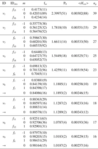
5. Period spacings and rotational splittings
From our list of significant independent frequencies we can
iden-tify 9 rotationally split doublets (ν1 – ν9 in Fig. 6), which
indi-cates that all modes have the same spherical degree of l = 1. Our mode identification is summarised in Tab. 4, where we as-sume symmetric triplets with the unobserved (i.e., unresolved) central (m = 0) component being located half way between the
|m| = 1 components. There are obviously some modes
miss-ing so that measurmiss-ing the period spacmiss-ing is not straightforward.
If we define the period spacing as dPi = 1/νi−1 −1/νi and
assume that between ν5 and ν6 two modes are missing (i.e.,
dP6 ≃ [1/ν5−1/ν6]/3) we find the period spacings presented
in Fig. 7 as solution S1. There is a strong gradient of dP with
the period, which is not consistent with theory (e.g. Miglio et al.
2008). A more realistic solution (S2in Fig. 7) is found when
as-suming 3 modes missing between ν5and ν6and one mode
miss-ing between ν2 – ν3, ν3 – ν4, and ν4 – ν5. The resulting period
spacings are quite uniform with only small deviations from the median value of about 5030 s, which is a typical value for a star like HD 201433 (see KIC 10526294; Pápics et al. 2014). Our as-sumption of filling missing modes might appear unrealistic but in fact alternating high- and low-amplitude modes were already observed in KIC 10526294, so that it is not surprising that some modes between detected modes fall below the detection limit of our observations (∼0.5 ppt). In Fig. 6 we show predictions of the mode sequences based on both solution but note that we cannot distinguish between them based on the observations alone.
The average rotational splittings are determined as <δfrot>=
(ν+1 − ν−1)/2 (with the indices of ν indicating the m value
of the mode). This means that we again assume symmetric triplets, which contradicts the findings of Pápics et al. (2014), but given the missing m = 0 components this is the only pos-sibility we have. Our splittings are, however, similar to what was reported for KIC 10526294 and have an average value of
∆ f =0.0028 d−1. Even the trend of increasing splittings towards
higher periods can be observed (bottom panel in Fig. 7), which implies a non-rigid internal rotation profile of the star. For solid body rotation the rotational splitting of l = 1 gravity modes is equal to half the rotation rate of the star, so that we can estimate the average rotation period of HD 201433 to be about 177 d. Since the assumption of a solidly rotating star is likely wrong, this value represents the average rotation period dominated by the near-core region, where the g modes have the largest contri-bution to the splittings.
0.004 0.003 0.002 δ frot (d -1 ) 2.5 2.0 1.5 1.0 Period (d) 10000 8000 6000 4000 Period spacing (s) ν9 ν8 ν7ν6 ν5 ν4 ν3
Fig. 7.Measured period spacings (top) and rotational split frequencies (bottom). The period spacings are shown for two different solutions (see text). While for S1(open squares) dPi =1/νi−1−1/νiis plotted as ob-served (only for ν6the measured spacing is divided by 3), for S2(filled circles) we divide the measured spacing for ν3−5by two and for ν6by 4 (ν7−9are the same as for S1). Diamond symbols (connected with a dashed line) represent period spacings of a representative MESA model. Triangle symbols in the bottom panel give the rotational splittings for KIC 10526294 (Pápics et al. 2014), where we exclude the two measure-ments with the largest uncertainties (for better visibility).
6. Coriolis/SMEI photometry of HD 201433
Even though the frequency doublets identified in the BTr data set represent a statistically solid result, as is demonstrated in Sec. 4, the separations of the individual components are close to the for-mal frequency resolution of the time series. Such a result might be considered at first glance questionable as it disagrees with the Loumos & Deeming (1978) criterion, which requires two close peaks to have a minimal separation of ∼1.5 times the frequency resolution to avoid influence on their apparent frequencies when applying the classical Fourier technique. In our case we have the fortunate situation that we can test our claims with a data set long enough to provide the required frequency resolution. These data are provided by the Solar Mass Ejection Imager (SMEI)
Table 4.Rotationally split triplets based on BTr and SMEI observations, In the case of BTr, the unresolved central (m = 0) component f0 is determined from the midpoint of the observed f±1components and P0 is the corresponding period. The split frequency <δfrot>is then half the difference between the m = 1 and m = −1 component and ng gives the radial order of the best-fit model frequency (see Sec. 7). In the case of SMEI (labeled by an arrow in the first column), f0 and <δfrot>are determined from a Lorentzian fit to the data. Frequencies and periods are given in units of d−1and d, respectively.
ID IDobs m fm P0 <δfrot> ng f15 -1 0.4173(11) ν1 0 0.42031(89) 2.3997(51) 0.00302(88) 39 f16 1 0.4234(14) f13 -1 0.55775(38) ν2 0 0.56125(32) 1.7818(10) 0.00351(33) 29 f14 1 0.56476(52) f9 -1 0.59867(30) ν3 0 0.60201(50) 1.6611(14) 0.00333(50) 27 f10 1 0.60535(92) f17 -1 0.6440(13) ν4 0 0.64727(75) 1.5449(18) 0.00325(71) 25 f18 1 0.65052(73) f7 -1 0.69813(32) ν5 0 0.70132(56) 1.4259(11) 0.00319(54) 23 f8 1 0.7045(11) f1 -1 0.83881(9) ν6 0 0.84139(10) 1.1885(1) 0.00258(10) 19 f3 1 0.84398(17) → 0 0.84086(16) 1.1893(2) 0.00246(15) f3 -1 0.88363(29) ν7 0 0.88597(16) 1.1287(2) 0.00233(16) 18 f4 1 0.88831(14) → 0 0.88578(13) 1.1289(2) 0.00243(12) f11 -1 0.92511(63) ν8 0 0.92706(36) 1.0787(4) 0.00193(36) 17 f12 1 0.92901(31) f5 -1 0.97975(10) ν9 0 0.98203(15) 1.0183(2) 0.00229(15) 16 f6 1 0.98431(29) → 0 0.98164(15) 1.0187(2) 0.00257(16)
on board the Coriolis satellite (Eyles et al. 2003; Jackson et al. 2004).
SMEIcomprises three wide-field cameras, which are aligned
such that the total field of view is a 180 deg and about 3 deg wide arc, so that a near-complete image of the sky is obtained after about every 102 min orbit. A detailed description of the data analysis pipeline used to extract light curves from these data is provided by Hick et al. (2007). The data of HD 201433 were
taken from the SMEI website7 and contain about 33 400
mea-surements covering almost eight years of near-continuous obser-vations. The classical frequency resolution therefore is ten times better than the frequency splittings which we are discussing for HD 201433 (see Tab. 4). Details about the data set are given in Tab. 1. 7 http://smei.ucsd.edu/new_smei/index.html 20 15 10 5 0 20 10 0 2.0 1.5 1.0 0.5 0.0 15 10 5 0 Amplitude (ppt) 5 4 0.95 0.90 0.85 20 15 10 5 0 Amplitude (ppt) Frequency (d-1) Time (1000d)
Fig. 8.Fourier amplitude spectrum of the SMEI data set of HD 201433. The top panel gives the original spectrum (grey line) with the red and blue lines indicating the significant frequenices in the BTr data set (Tab. 2) and their mid-point, respectively. The insert shows the full fre-quency range. The middle panel shows the same spectrum along with a sequence of Lorentzian profiles (red line) fitted to the spectrum. The bottompanel shows the (color-coded) amplitude at the central frequen-cies of the Lorentzians as a function of time. The amplitudes are de-termined within a 720 d long subset moved across the full time series in 100 d steps. The horizontal dotted lines separate fully independent parts.
The SMEI photometric time series are subject to strong in-strumental effects, such as large yearly flux fluctuations, which obviously are due to an insufficient background correction. As a remedy we phased the data with a period of one year and com-puted the median flux in 200 phase sub-intervals and find an an-nual amplitude of about 0.8 mag. We applied an Akima spline fit and computed the residuals to the smooth one-year variation. Back in the time domain one sees outliers, jumps, irregular inten-sity changes and low frequency variations in the residuals which have to be removed in order to make the very low amplitude fre-quencies in question detectable. This “cleaning" was achieved via iterative spline interpolation anchored on the median flux in 2–3 day intervals (in other words applying a high–pass filter) by 3–5 σ clipping to remove outliers and repeating this procedure 20 times. As a result of this rather arbitrary procedure any signal is gradually suppressed towards low frequencies.
The resulting SMEI time series of HD 201433 is homoge-neously sampled without significant aliasing. The median ca-dence of about 101.6 min results in a Nyquist frequency of
∼7 d−1, which is high enough to cover the intrinsic variability
of HD 201433. The Fourier amplitude spectrum of the SMEI data set is shown in Fig. 8. Compared to the BTr spectrum, the formal frequency resolution is more than 18 times better
(∼0.00035 d−1compared to 0.0064 d−1 for the BTr data), while
the noise level in the Fourier domain is obviously much higher (∼0.53 ppt compared to 0.11 ppt in the BTr data). The photo-metric precision is, however, sufficient to clearly detect the three
obser-vations. In fact, the doublets turn out to be triplets with the cen-tral component having a smaller (or comparable) amplitude than the wing components. This clearly indicates that the BTr obser-vations are not long enough to resolve all three components of the intrinsic triplets even when using our present frequency anal-ysis method. The frequencies (and even the amplitudes) of the wing components (red vertical lines in the top panels of Fig. 8) agree well, however, with the signal found in the SMEI spec-trum. Also the central components, which were estimated from the midpoints of the (BTr) wing components, are in good agree-ment.
To quantify the agreement we tried to extract the individ-ual frequencies from the SMEI observations but find a classical pre-whitening sequence to be insufficient as the individual fre-quencies split up in many components indicating strong ampli-tude modulations. This is already visible in the actual spectrum showing multiple side-lobes around the expected positions of the frequencies. Such a structure reminds of the pattern of intrinsi-cally damped and stochastiintrinsi-cally excited modes (so-called solar-like oscillations) produce in the Fourier spectrum. This is why we fit a sequence of three Lorentzian triplets to the spectrum,
P( f ) = P0+X n 1 X m=−1 hnζm(i) 1 + 4 [πτ ( f − fn−m · δ frot,n)]2 , (1)
where P is the Fourier power, fn is the frequency of the central
component of the n-th triplet and δ frot,nis its rotational splitting.
For simplicity we use a single lifetime parameter τ for all modes.
The mode height hnscales with a geometric factor ζm(i), which
depends on m and the inclination i at which the pulsation axis is seen. According to Gizon & Solanki (2003) this geometric
fac-tor is cos2ifor the m = 0 component and 0.5 sin2ifor the |m| = 1
components of a dipole mode. More details about the detec-tion of Lorentzian profiles are given by, e.g., Gruberbauer et al. (2009). We again use MultiNest for the fit and find a best-fit
inclination and mode lifetime of 68±5◦and 680±110 d,
respec-tively. The central mode frequencies and rotational splittings are listed in Tab. 4 and the best-fit sequence of Lorentzian triplets is shown in the middle panels of Fig. 8. The triplets at about 0.88
and 0.98 d−1 are well defined so that we can test the
assump-tion of symmetric splittings for them. A fit with a modified Eq. 1 (where we allow for individual splittings) indeed shows that the wing components are equally separated from the central compo-nent within the uncertainties of about 5%.
We emphasise here that it does not necessarily mean that modes have indeed a stochastic nature, if Lorentzians work well in extracting the mode frequencies from the SMEI observations. In fact, this is very difficult to prove, because one has to show that the signal phase is not coherent, which requires continuous observations that cover many lifetime cycles of the mode. The
SMEI data cover about five lifetime cycles (if the modes were
stochastic), which is likely not enough to verify a stochastic na-ture. We do, however, find a strong amplitude modulation for the individual frequencies. To quantify this we fit a sine function to a 720 d long subset of the time series, where we fix the frequency to the value determined earlier by the Lorentzian fit. Moving the subset across the SMEI data in steps of 100 d gives the amplitude (and phase) of a given frequency as a function of time. This is shown in the bottom panel of Fig. 8. We tested various window sizes but always find the same general behaviour. The strongest
modulation is found for the triplet at about 0.84 d−1. While the
amplitude of the central component is fairly constant, the wing components vary in amplitude by a factor of more than four. Also interesting is that the variations are periodic with a timescale of
about 1 500 d and that they are in anti phase. The amplitude min-imum of the m = −1 component coincides approximately in time with the largest amplitude of the m = +1 component, and vice versa. A similar but less pronounced behaviour can be found for
the triplet at about 0.98 d−1. Only the triplet at 0.88 d−1 is
dif-ferent. The timescale of its modulation is much longer and the wing components vary approximately in phase. The physical ori-gin for this phenomenon is unknown to us but we note that some-thing similar is seen in the Kepler observations of KIC 10526294 (Pápics et al. 2014). Even though the authors did not follow up on this, many modes illustrated in their Fig. 9 show a multiple peak structure typical for amplitude modulation.
Apart from the three triplets shown in Fig. 8 and a single
sharp peak at 0.40013 d−1(for which we have no explanation at
this point) we do not find any further significant variability in the
SMEIdata. The data set does, however, allow us to verify several
assumptions made during the analysis of the BTr observations:
– Our interpretation of the nine pairs of close frequencies in the
BTr data as symmetrically split doublets is confirmed by the independent SMEI observations. Even though we can only verify the three largest-amplitude multiplets, the remaining doublets follow the same statistical criteria and only their amplitudes are smaller, but still significant in the BTr time series.
– The frequencies of the central components and rotational
splittings agree on average within ∼1.8 σ and 0.8 σ, respec-tively, between BTr and SMEI.
– The interpretation of individual frequencies extracted from
the BTr observations as independent oscillations requires ap-proximately stable signal amplitudes. Even though we defi-nitely find amplitude modulations, their timescales are long enough to consider the oscillations in first approximation to be stable during the 156 d long BTr observations. Even for shorter lengths of the subsets, which are used for the bot-tom panel of Fig. 8, we do not find evidence for significant amplitude modulations shorter than those mentioned above.
– The amplitude modulations also provide a reasonable
expla-nation for the missing modes (Sec. 5) as it might well be that their amplitudes were below the detection threshold of the BTr observations.
Finally we note that we cannot straightforwardly constrain the inclination angle of HD 201433 since the observed frequen-cies are heat-driven modes. In this case, the 2l + 1 compo-nents of a rotationally split non-radial mode are not excited to the same amplitude, contrary to solar-like oscillators (e.g. Gizon & Solanki 2003). However, the formally best-fit value of
68±5◦gives an amplitude ratio between the central and wing
components which is at least not inconsistent with the observed ones. It seems to be plausible that we see the star more equator-on than pole-equator-on.
7. Asteroseismic analysis
To interpret the observed rotational splittings in terms of inter-nal differential rotation we need a representative stellar model for HD 201433. We therefore compare the observed g modes to non-adiabatic pulsation modes computed with the GYRE stellar oscillation code (Townsend & Teitler 2013) for a grid of non-rotating equilibrium stellar models along stellar evolutionary tracks that pass through the spectroscopic error box (see Tab. 7 and Sec. 1). The models are calculated with the MESA stellar structure and evolution code (Paxton et al. 2011, 2013). As we
Fig. 9.Visualisation of the multi-dimensional χ2(left axis; black sym-bols) and probability (right axis; grey symsym-bols) space that results from the comparsion of the observed and computed MESA/GYRE modes. Red circles mark the two best-fit models.
are for the time being only interested in a representative model we restrict the models to a single initial chemical composition of (Y, Z) = (0.28, 0.02) and turn off convective core overshooting. We evolve a set of zero-age main-sequence models with masses
ranging from 2.9 to 3.225 M⊙(with steps of 0.025 M⊙) until their
core hydrogen mass fraction drops below Xc=0.3. To achieve
sufficient resolution along the tracks we limit the evolutionary time steps to 0.2 Myr, which results in about 5 200 models with
a typical resolution in Xcof 0.002 close to the ZAMS to 0.004
for the most evolved models.
We then compute l = 1 modes with non-adiabatic
fre-quencies ranging from 0.3 to 1.2 d−1. To search for a best-fit
model we compare the observed frequencies (νobs) to the
the-oretical ones (νmodel) by computing the reduced χ2 value (e.g.
Pamyatnykh et al. 1998; Guenther & Brown 2004),
χ2= 1 N N X i=1 (νi,obs− νi,model)2 σ2i,obs+ σ2model , (2)
where N and σobsare the total number of observed modes and
their frequency uncertainties. The typical numerical uncertainty
of the model frequencies (σmodel) is estimated from following
the frequency of a specific mode (i.e., with a given radial order) during stellar evolution. We thereby assume the actual numer-ical uncertainty to be of the order of the point-to-point scatter after subtracting a running average. We find a value of about
0.00003 d−1, which is comparable to σ
obs in some cases and
therefore not negligible.
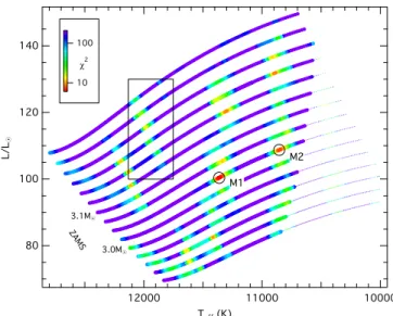
The resulting multi-dimensional χ2space is shown in Fig. 9
and illustrates that while the grid resolution along the evolution-ary tracks is sufficient (indicated by the smooth decrease and
increase of χ2 around the best-fit model when plotted, e.g., as
140 120 100 80 L/L 8 12000 11000 10000 Teff (K) 10 100 χ2 3.0M8 3.1M8 ZAMS M1 M2
Fig. 10.HR diagram showing the model grid that is used to search for a representative stellar model of HD 201433. The models are color-coded according to their χ2 value and shown with thick lines when at least one mode excited (i.e., with a positive work integral) and with thin lines when all modes are damped. The two best-fit models are marked with black circles. The black rectangle indicates the spectroscopic error box (see Tab. 7 and Sec. 1).
a function of R) the resolution in mass is still too low to find a model whose frequencies agree within the observational un-certainties. We can, however, identify a model that fulfils our requirements (approximately representing the internal structure
of HD 201433). The best-fit model has a χ2value of about 6.3,
which means that its frequencies matches the observed ones on average within 2.5 (i.e., square root of 6.3) times the average observational errors. The best-fit model parameters are listed in Tab. 5 and its frequencies and period spacings are compared to the observational values in Fig. 6 and 7, respectively. We fur-ther note that increasing the mass resolution would not allow us to improve the situation without simultaneously computing models with various chemical compositions and convective core overshoot parameters. Pápics et al. (2014) and Moravveji et al. (2015) found strong correlations between the mass, the over-shoot parameter, and the chemical composition in their seis-mic analysis of KIC 10526294 (a star that is very similar to HD 201433 in mass and chemical composition, but less evolved), from which we can estimate that turning on core overshooting could potentially increase the mass of the best-fit model by up to
0.1 M⊙. They do, however, also find that models with a low
over-shoot parameter fits the observations best. Also the fact that our best-fit model is outside the expected range from spectroscopy in the HR diagram (see Fig. 10) is not really troubling since chang-ing the chemical composition would again slightly change the mass and therefore the position in the HR diagram.
A disadvantage of the χ2 method is its inability to
pro-vide uncertainties and therefore to set a limit on which models (within the grid) represent the observations and which do not. The “second-best”-fit model M2 (with its position in the HR
di-agram significantly different from M1) has a χ2 of about 7.85
and therefore fits the observed frequencies marginally less well. We therefore follow the approach of Kallinger et al. (2010) to determine the Bayesian model probability and find that for our model grid about 99.9% of the total probability is concentrated in the close vicinity (about ±15 K) of the best-fit model M1 (M1
1.0 0.8 0.6 0.4 0.2 0.0 º r Knl (r) dr / º R K nl (r) dr 1.0 0.8 0.6 0.4 0.2 0.0 m/M ν9 ν8 ν7 ν6 ν5 ν4 ν3 ν2 ν1 1.0 0.8 0.6 0.4 0.2 0.0 m/M 1.0 0.8 0.6 0.4 0.2 0.0 r/R
Fig. 11. Normalised integrated rotational kernels for the nine dipole modes in model M1 representing best the observed frequencies in HD 201433. The insert shows how the mass is distributed in the model. The vertical dashed lines represent the boundaries of the sharp spike in the Brunt-Väisälä frequency (see Fig. 12) with the inner one marking the boundary of the convective core.
itself has a p of about 0.15) and that there is only a marginal probability that M2 provides the best representation of the ob-servations (see Tab. 5). Even though this would already rule out M2 we further investigate it in order to check if a slightly dif-ferent internal structure (M2 is more evolved than M1 and has a smaller relative core size) affects the further analysis.
8. Internal rotation profile
Building on the measurements of Pápics et al. (2014) for KIC 10526294, Triana et al. (2015) provided the first internal rotation profile of an unevolved intermediate-mass B-type star. They found the star to rotate near its core-envelope boundary with a period of about 71 d and while their seismic data point towards a counter-rotating profile within the radiative envelope they cannot rule out rigid rotation. Such results are key to tackle one of the big open questions in stellar evolutionary theory: the transport of angular momentum inside stars. With the nine ro-tationally split g modes identified in HD 201433 we are able to provide another example of an internal rotation profile for a star very similar to KIC 10526294.
If we assume that the cyclic rotation frequency Ω depends
only on the radial coordinate r, then the frequency splitting δfrot
Table 5.Properties of the two best fitting models. See text for details. Teff is given in K, M, L, and R in solar units, and the age in Myr. The hydrogen mass fraction in the core Xcis given in units of 1.
Teff M L R χ2 p log g Xc age M1 11363 3.05 100.4 2.589 6.30 0.15 4.096 0.464 145 M2 10854 3.05 108.7 2.953 7.85 1.5e-4 3.982 0.338 199
of a mode with degree l and radial order n can be written as, δfrot(n, l) = 1 2πIn,l Z R∗ 0 Kn,l(r)Ω(r)dr, (3)
where In,l is the mode inertia and Kn,l(r) gives the unimodular
mode kernel, that is a function of the mode’s displacement
am-plitudes (e.g. Cox 1980). R∗is the radius of the model.
Normalised integrated versions of the rotation kernels of HD 201433 are given in Fig. 11 and basically show how a rota-tionally split frequency is accumulated throughout the star. Ob-viously, different modes are more or less sensitive to rotation in
different regions of the star. The mode ν9, e.g., gains about 10%
of its frequency splitting from rotation in the thin layer above the
convective core, where N2spikes (see Fig. 12). The mode ν
7, on
the other hand accumulates almost three times more of its rota-tional splitting in the same region. This “differential” sensitivity to different parts of the star allow us to resolve the stellar rotation profile.
From the fact that the modes ν7 and ν9have practically the
same observed rotational splitting we can already conclude that HD 201433 is either a rigid rotator or it rotates much faster in the outer layers than the inner ones (because otherwise the split
frequencies of ν7 and ν9 would be different). Several inversion
techniques have been developed in the past aiming to determine the internal rotation profile of the Sun. The inversion of Eq. 3 is, however, a highly ill-conditioned problem that requires, e.g., numerical regularisation. Beck et al. (2014) found that classi-cal approaches like the RLS method (e.g. Christensen-Dalsgaard 1990) or the SOLA technique (e.g. Schou et al. 1998) are not well-suited for stars with only a few observed rotational split-tings (like red giant stars, but also SPB stars) and easily become numerically unstable or it is very difficult to evaluate the accu-racy and especially the reliability of the result.
8.1. Forward-modelling of the rotation profile
We therefore follow the forward modelling approach developed by one of us (TK in Beck et al. 2014). The algorithm computes synthetic rotational splittings for a parameterised rotation profile and compares them to the observed splittings. The form of the
20x10-6 15 10 5 0 S 2, N 2 (s -2) 1.0 0.8 0.6 0.4 0.2 0.0 r/R 10-10 10-9 10-8 10-7 10-6 10-5 1.00 0.98 0.96 0.94 0.92 0.90 0.88 ν9 ν1
Fig. 12.Squared Brunt-Väisälä N2(solid lines) and Lamb S2(dashed lines) frequency as a function of the fractional radius for model M1 (black lines) and M2 (grey lines). The blue lines indicate regions where N2is negative, and are therefore convective. The insert shows the out-ermost region and the frequency range of the observations (grey-shaded area between the red lines).
profile is thereby very flexible. One can, e.g., implement a lin-ear piece-wise model or a functional form (like a Gaussian or a polynomial). The profile parameters are again fitted with the Bayesian nested sampling algorithm MultiNest. These
parame-ters are Ωnin the case of a zonal model with n zones, or the
co-efficients of a chosen function. The advantage of this approach is again to provide realistic uncertainties and its capability to compare different models and rate which one best represents the observations (e.g., differential rotation vs. rigid rotation). The algorithm was developed to handle the few available rotational splittings in red giants and has proven to give reliable results that are fully consistent with other methods (e.g. Beck et al. 2014, Beck et al., in prep.).
The modes that are accessible to our analysis probe the radia-tive envelope of HD 201433 from the boundary of the convecradia-tive core (at a radius and mass fraction of ∼0.11 and 0.15,
respec-tively) up to about r = 0.98R∗(m > 0.9999M∗), above which all
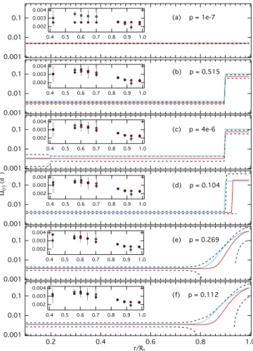
frequencies fall above the Lamb frequency (see Fig. 12), which sets the upper limit for g modes to propagate. We can therefore not expect to directly get information about the core rotation rate and the outer ∼2% of the star. We tried various models for the tation profile to fit the observed splittings, ranging from rigid ro-tation, over linear piece-wise models (with up to 9 zones), poly-nomial functions, Gaussians, multi-Gaussians, to Lorentzian and error functions. A selection of the resulting rotation profiles are shown in Fig. 13 and more details are given below:
(a) Rigid rotation: Assuming rigid rotation we find a rotation
pe-riod of 201±5 d ( ˆ= 0.0050±0.0001d−1). However, as can be
seen in the insert of panel (a) in Fig. 13, the synthetic split-tings that result from integrating the mode kernels, folded with the rotation profile, do not fit the observed splittings at all. In comparison with other fits the model probability of
about 10−7 is extremely low. We can therefore rule out an
entirely rigidly rotating radiative envelope for HD 201433. (b) and (c) Multi-zonal rotation profiles: We test various zonal
models with a fixed position of the zone boundary, i.e., “hard-wired” in the model and find the best formal model probability (p = 0.515) for a fit with a two-zone model with the zone boundary set at a radius fraction of 0.9 (panel (b) in Fig. 13). The inner and outer zones rotate with
a period of 314±43 d−1( ˆ= 0.0033±0.0005d−1) and 14±3 d
( ˆ= 0.076±0.018 d−1), respectively. We do not find another
model, even with more zones, that comes close in model probability. As an example we show a three-zone model in
panel (c) of Fig. 13, where we add an inner zone (0 - 0.2R∗)
but find it to rotate with practically the same rotation rate as the middle zone. This indicates that the data do not support differential rotation in the radiative envelope of HD 201433 below a radius fraction of about 0.9. The very low model probability compared to model (b) results from the additional parameter in the fit8.
(d) Two-zone profile with variable zone boundary: In a next step we tried to locate the transition region between the inner slow and outer fast rotating zone. In contrast to the fixed location of the zone boundary in the original two-zone model we now leave it as a free parameter in the fit. The result is shown in panel (d) locating the zone boundary at a radius fraction
of r/R∗ =0.93±0.02. While the rotation period of the inner
8 Roughly spoken, in a Bayesian concept a model gets assigned a penalty for its complexity so that a model with n + 1 parameters has to fit the data significantly better than a model with n parameters to get assigned the same (or even higher) model evidence. More details are provided by Jeffreys (1998). 0.001 0.01 0.1 0.004 0.003 0.002 1.0 0.9 0.8 0.7 0.6 0.5 0.4 0.001 0.01 0.1 0.004 0.003 0.002 1.0 0.9 0.8 0.7 0.6 0.5 0.4 0.001 0.01 0.1 0.004 0.003 0.002 1.0 0.9 0.8 0.7 0.6 0.5 0.4 0.001 0.01 0.1 0.004 0.003 0.002 1.0 0.9 0.8 0.7 0.6 0.5 0.4 0.001 0.01 0.1 0.004 0.003 0.002 1.0 0.9 0.8 0.7 0.6 0.5 0.4 Ω(r) (d -1 ) r/R* (a) p = 1e-7 (b) p = 0.515 (c) p = 4e-6 (d) p = 0.104 (e) p = 0.269 0.001 0.01 0.1 1.0 0.8 0.6 0.4 0.2 0.004 0.003 0.002 1.0 0.9 0.8 0.7 0.6 0.5 0.4 (f) p = 0.112
Fig. 13.Internal rotation profiles from our forward-modelling approach using various models (panel (a): constant rotation; (b): two-zone model with fixed zone boundary; (c): three-zone model with fixed boundary; (d): two zone model with variable zone boundary; (e): Gaussian pro-file centered at the surface; (f ): error function propro-file). Red and blue lines indicate rotation profiles resulting from mode kernels of the best-fit models M1 and M2, respectively. The uncertainties (black dashed lines) are only plotted for M1-based profiles for better visibility but are similar for the M2-based profiles. The inserts show the observed (grey symbols) and best-fit (red symbols) rotational splittings as a function of the mode frequency with the axes in d−1.
zone remains almost the same, the outer zone now rotates with a period of about 5.5 d ( ˆ= 0.182 d−1) significantly faster
than for the original two-zone model. However, due to the ro-tational splittings containing less and less information about rotation when approaching the surface, the uncertainties start to dramatically increase.
(e) Gaussian rotation profile: So far, the analysis points towards a slowly and rigidly rotating zone that contains almost the en-tire mass of the radiative envelope, topped by a thin and sig-nificantly more rapidly rotating surface layer. The assump-tion of a sudden increase in rotaassump-tion speed (by a factor of 20 or so) at the zone boundary seems, however, physically not very plausible. We therefore use a Gaussian rotation pro-file in which it turns out that we get the best results (i.e., the best model probability) when fixing the centre of the Gaussian to the stellar surface. While the inner rotation
pe-riod of 292±76 d ( ˆ= 0.0034+0.0012
−0.0007d−1) agrees well with the
two-zone models, the surface rotation rate is 0.30±0.21 d−1
( ˆ= 3.33+7.78