HAL Id: hal-02625960
https://hal.inrae.fr/hal-02625960
Submitted on 26 May 2020
HAL is a multi-disciplinary open access archive for the deposit and dissemination of sci-entific research documents, whether they are pub-lished or not. The documents may come from teaching and research institutions in France or abroad, or from public or private research centers.
L’archive ouverte pluridisciplinaire HAL, est destinée au dépôt et à la diffusion de documents scientifiques de niveau recherche, publiés ou non, émanant des établissements d’enseignement et de recherche français ou étrangers, des laboratoires publics ou privés.
A tool to guide the selection of impact categories for
LCA studies by using the representativeness index
Antoine Esnouf, Reinout Heijungs, Gustave Coste, Eric Latrille, Jean-Philippe
Steyer, Arnaud Helias
To cite this version:
Antoine Esnouf, Reinout Heijungs, Gustave Coste, Eric Latrille, Jean-Philippe Steyer, et al.. A tool to guide the selection of impact categories for LCA studies by using the representativeness index. Science of the Total Environment, Elsevier, 2019, 658, pp.768-776. �10.1016/j.scitotenv.2018.12.194�. �hal-02625960�
Version postprint
A tool to guide the selection of impact categories for
1
LCA studies by using the Representativeness Index
2
Antoine Esnouf a,b*, Reinout Heijungs c,d, Gustave Coste a,b, Éric Latrille a, Jean-Philippe Steyer
3
a, Arnaud Hélias a,b,e
4
5
a LBE, Univ Montpellier, , INRA, Montpellier SupAgro, Narbonne, France
6
b Elsa, Research group for Environmental Life cycle and Sustainability Assessment, Montpellier,
7
France 8
c Department of Econometrics and Operations Research, Vrije Universiteit Amsterdam,
9
Amsterdam, The Netherlands 10
d Institute of Environmental Sciences, Department of Industrial Ecology, Leiden University,
11
Leiden, The Netherlands 12
d Chair of Sustainable Engineering, Technische Universität Berlin, Berlin, Germany
13
14
*Corresponding author. LBE, Univ Montpellier, INRA, Montpellier SupAgro, 102 avenue des 15
Etangs, 11100, Narbonne, France. E-mail address: [email protected]. Tel.: +33 16
499612171. 17
Version postprint
ABSTRACT 18
Understanding the environmental profile of a product computed from the Life Cycle Assessment 19
(LCA) framework is sometimes challenging due to the high number of environmental indicators 20
involved. The objective here, in guiding interpretation of LCA results, is to highlight the 21
importance of each impact category for each product alternative studied. For a given product, the 22
proposed methodology identifies the impact categories that are worth focusing on, relatively to a 23
whole set of products from the same cumulated database. 24
The approach extends the analysis of Representativeness Indices (RI) developed by Esnouf et al. 25
(2018). It proposes a new operational tool for calculating RIs at the level of impact categories for 26
a Life Cycle Inventory (LCI) result. Impact categories and LCI results are defined as vectors within 27
a standardized vector space and a procedure is proposed to treat issues coming from the correlation 28
of impact category vectors belonging to the same Life Cycle Impact Assessment (LCIA) method. 29
From the cumulated ecoinvent database, LCI results of the Chinese and the German electricity 30
mixes illustrate the method. Relevant impact categories of the EU-standardised ILCD method are 31
then identified. RI results from all products of a cumulated LCI database were therefore analysed 32
to assess the main tendencies of the impact categories of the ILCD method. This operational 33
approach can then significantly contribute to the interpretation of the LCA results by pointing to 34
the specificities of the inventories analysed and for identifying the main representative impact 35
categories. 36
37
KEYWORDS: LCA, Life Cycle Inventory, Life Cycle Impact Assessment, representativeness, 38
dimension reduction, interpretation tools 39
Version postprint
1. Introduction
41
While the main goal of the Life Cycle Assessment (LCA) framework is to quantify and assess all 42
the potential environmental impacts of human activities (ISO, 2006), the study of results over a 43
too wide range of environmental impacts can become inefficient and lead to unclear conclusions 44
(Steinmann et al., 2016). To obtain those environmental impact results, the LCA framework is 45
structured in four phases where the Life Cycle Inventory (LCI) phase is one of the key one; it 46
describes a product, a process or an activity throughout its value chain and quantifies its system-47
wide emissions and resource extractions. An LCI database (of which ecoinvent (Wernet et al., 48
2016) is a prime example) contains a large number of unit processes, each of which specifies the 49
inputs and outputs (such as electricity, plastic, fossil resources and pollutants) of activities (such 50
as rolling steel or driving a truck). Those LCI unit process databases allow LCA practitioners 51
modelling the whole value chain of their study in reasonable time. The result of an LCI is a list of 52
quantified emissions and resource extractions, collectively indicated as elementary flows, 53
aggregated over all (up to thousands) unit processes that make up the system. In a cumulated LCI 54
database, the entries are not the unit processes but rather the system-wide elementary flows, for 55
each included product. From the LCI result, the Life Cycle Impact Assessment (LCIA) phase then 56
translates these elementary flows in terms of environmental impacts. Different LCIA methods are 57
available, often with a name, such as ReCiPe (Goedkoop et al., 2009), Traci (Bare, 2011) and 58
ILCD (EC-JRC, 2010a). Each LCIA method consists of a number of environmental impact 59
categories (such as global warming and ecotoxicity) and proposes Characterization Factors (CFs) 60
to quantitatively link the elementary flows to these impact categories. There are often ten or more 61
such impact categories within each LCIA method (EC-JRC, 2010b). Although aiming at being 62
Version postprint
holistic, such large sets of impact categories can challenge the efficiency of environmental 63
regulations (like product eco-design, decision making or environmental labelling). Further 64
modelling the impacts into so-called endpoint damage levels could resolve the issue related to 65
large sets. However, due to uncertainties, all models which are presently available are still 66
classified as “interim” (Hauschild et al., 2013). 67
A reduction in the number of impact categories, by selecting the most relevant impact categories 68
to focus on, would enable more effective environmental optimization. For comparative LCA, 69
existing practices for normalization and weighting use external valuation of impact categories that 70
might guide LCA practitioners on a reduced subset of LCIA results to interpret (Lautier et al., 71
2010). However, these procedures are increasingly discouraged (Prado-Lopez et al., 2014). By 72
quantifying the uncertainties, exploration of the relative importance of impact categories through 73
the magnitude of differences between LCIA results can produce promising tools for comparative 74
LCA (Mendoza Beltran et al., 2018). 75
Some authors used Principal Component Analysis (PCA), combined with uncertainty analysis or 76
multi-objective optimization (Mouron et al., 2006; Pozo et al., 2012) to deal with the large number 77
of environmental indicators. Sometimes, PCA was also applied on LCIA results with technical 78
indicators to reveal the relationships between those indicators (Basson and Petrie, 2007; Bava et 79
al., 2014; Chen et al., 2015; De Saxcé et al., 2014). 80
Steinmann et al. (2016) applied PCA over a large range of products and LCIA methods (all the 81
LCIA results of 135 impact categories for 976 products provided by ecoinvent) to select impact 82
categories. In order to deal with impact category units and the wide orders of magnitude of LCIA 83
results due to the high diversity of reference flows, they proposed to apply a product ranking. An 84
Version postprint
alternative approach was a log-transformation on LCIA results prior to using a multi-linear 85
regression (Steinmann et al., 2017). As comment to this last article, Heijungs (2017) noticed that 86
the reference flow values of the studied LCIA results affect the outcomes of their work. He 87
suggested standardizing the LCIA results by their energy footprint to be free of the default 88
reference flow. This emphasizes the need to address data heterogeneity. 89
Other studies that apply multivariate statistical analysis or multi-linear regression on LCIA results 90
of products from ecoinvent focus on revealing correlation or alleged redundancies between impact 91
categories (Huijbregts et al., 2006; Pascual-González et al., 2016, 2015; Steinmann et al., 2017). 92
The objectives of these studies were to predict LCIA results from a reduced number of proxy 93
impact categories. All these approaches work on the impact category results alone, and do not 94
consider LCI information and its translation to impact categories. 95
By translating the elementary flows in terms of impact categories, LCIA can be considered to be 96
a dimension reduction technique: LCIs are described by LCI results with more than a thousand 97
variables (elementary flows) while LCIA results are a much smaller number of environmental 98
indicators. The remaining dimensions, which all have an environmental meaning, may not all be 99
necessary for dealing with the main environmental issues of the studied product. As the 100
environment is disturbed and even damaged by such diverse substance emissions or resource 101
utilizations from different human activities, all impact categories should be covered, but some of 102
them may not be essential for the conclusion of one particular product, for instance, because they 103
are strongly correlated with other impact categories. 104
The Representativeness Index (RI) was recently proposed by Esnouf et al. (2018) to provide a 105
relative measure of the discriminating power of LCIA methods. The RI is meant to explore the 106
Version postprint
relative relevance of each impact category belonging to a LCIA method for a specific product. It 107
does not assess the relevance of the environmental model behind impact categories of the LCIA 108
methods, but it is an aid to LCA practitioners, so they might focus on a reduced number of impact 109
categories that best represent the elementary flows associated with a particular product. Moreover, 110
by studying the links between the RI of an entire LCIA method and the RIs of its constituent impact 111
categories, some issues have been raised on the correlation of the representativeness of impact 112
categories (Esnouf et al. (2018). 113
The aim of this paper is to further develop the potential benefits of the RI methodology and to 114
discuss representativeness issues regarding non-orthogonal (i.e. dependent) impact categories, and 115
ways to solve such issues. We also developed an operational tool to calculate RIs as a 116
downloadable Python package from an open access deposit. 117
The present paper is organized as follows: in Section 2, the standardization of the vector space 118
where the LCA study takes place and the proximity relationship between an LCI vector and LCIA 119
method subspaces (or impact category vectors) is briefly revisited as it is the same framework as 120
that explained in Esnouf et al. (2018). The algorithm of orthogonalization of impact categories to 121
avoid redundancy issues within a LCIA method is presented. The approach is illustrated and 122
discussed in Section 3 on the ILCD method for two products results from the cumulated ecoinvent 123
database (Wernet et al., 2016). Main tendencies of RI results over the cumulated LCI database are 124
then explored. The main representative dimensions that support most of the RI values are then 125
determined. Finally, results from the decorrelation algorithm are analysed over the entire 126
cumulated LCI database. 127
2. Material and method
Version postprint
Table 1 lists notations that are used in the present work. Vectors and matrices are distinguished 129
from scalar by being written in bold, matrices are moreover capitalized. 130
Table 1. List of symbols and their meaning
131
Symbol Meaning
𝑚 Number of products in LCI database 𝑛 Number of elementary flows
𝑝 Number of impact categories in a LCIA method 𝐠𝑖 LCI result vector of the 𝑖th product (𝑖 = 1, … , 𝑚)
𝑔𝑥,𝑖 The amount of the 𝑥th elementary flow for the 𝑖th product (𝑖 = 1, … , 𝑚; 𝑥 = 1, … , 𝑛)
𝐪𝑗 The vector of characterization factors of the 𝑗th impact category: an impact category
vector (𝑗 = 1, … , 𝑝)
𝑞𝑥,𝑗 The characterization factor of the 𝑗th impact category for the 𝑥th elementary flow
(𝑗 = 1, … , 𝑝; 𝑥 = 1, … , 𝑛)
𝐐 LCIA method matrix composed of a set characterization vectors of 𝑝 impact categories
ℎ𝑗,𝑖 LCIA result of the 𝑖th product on the 𝑗th impact category (𝑖 = 1, … , 𝑚; 𝑗 = 1, … , 𝑝)
𝐺𝑥 Geometric mean of 𝑔𝑥,𝑖 for the 𝑥th elementary flow (𝑥 = 1, … , 𝑛)
𝐠̃𝑖 Standardized form of 𝐠𝑖 (using the geometric mean) (𝑖 = 1, … , 𝑚)
𝐪
̃𝑗 Standardized form of 𝐪𝑗 (using the geometric mean) (𝑗 = 1, … , 𝑝)
𝐐̃ LCIA method matrix consisting of standardized impact vectors 𝐪̃𝑗 𝛾𝑗,𝑖 Angle between 𝐪̃𝑗 and 𝐠̃𝑖 (𝑖 = 1, … , 𝑚; 𝑗 = 1, … , 𝑝)
𝐪
̃𝑗⊥ Orthogonalized form of 𝐪̃𝑗 (from a Gram-Schmidt process) (𝑗 = 1, … , 𝑝) 𝐐̃⊥ LCIA method matrix consisting of orthogonalized impact vectors 𝐪̃
𝑗 ⊥
𝑅𝐼𝑗,𝑖 Representativeness index of 𝐪̃𝑗 for 𝐠̃𝒊 (𝑖 = 1, … , 𝑚; 𝑗 = 1, … , 𝑝)
𝑅𝐼𝑖 Representativeness index of LCI-result 𝐠̃𝒊 for all impact categories (𝑖 = 1, … , 𝑚)
𝑅𝐼𝑗,𝑖⊥ Ortohogonal representativeness index of 𝐪̃𝑗⊥ for 𝐠̃𝒊 (𝑖 = 1, … , 𝑚; 𝑗 = 1, … , 𝑝)
𝑅𝐼𝑖⊥ Orthogonal representativeness index of LCI-result 𝐠̃𝒊 for all orthogonalized impact
categories (𝑖 = 1, … , 𝑚)
𝑅𝐼𝑗,𝑖decorr Decorrelated representativeness index of 𝐪̃𝑗 for 𝐠̃𝒊 (𝑖 = 1, … , 𝑚; 𝑗 = 1, … , 𝑝)
𝑆𝑅𝑅𝑗 Sum of squared correlation coefficients of 𝐪̃𝑗 and all other 𝐪̃-vectors (𝑗 = 1, … . , 𝑝)
Θ𝑗 A set of impact category vectors that are correlated to 𝐪𝑗 and belonging to 𝐐 (𝑗 = 1, … , 𝑝)
𝑆𝑖 Sum of squared RIs over 𝑡 = 1, … , 𝑝 (𝑖 = 1, … , 𝑚)
Version postprint
𝑅𝑡,𝑖,𝑘 RI result of the 𝐪̃𝑡 for 𝐠̃𝑖 and treated during the iteration 𝑘 (𝑡 = 1, … , 𝑝; 𝑖 =
1, … , 𝑚; 𝑘 = 2, … , 𝑝)
𝑑𝑗,𝑖 Distance between 𝑅𝐼𝑗,𝑖 and 𝑅𝐼𝑗,𝑖⊥ (𝑖 = 1, … , 𝑚; 𝑗 = 1, … , 𝑝)
〈𝐱, 𝐲〉 Inner product of vectors 𝐱 and 𝐲 ‖𝐱‖ Norm (Euclidean length) of vector 𝐱 132
2.1. RI methodology
133
2.1.1. Standardization and definition of an inner product 134
As proposed by several authors (Esnouf et al., 2018; Heijungs and Suh, 2002; Téno, 1999) the 135
vector space where the LCA framework takes place is generated by a basis that represents the n 136
elementary flows that are included in the study. The result of the LCI phase, for the 𝑖th product,
137
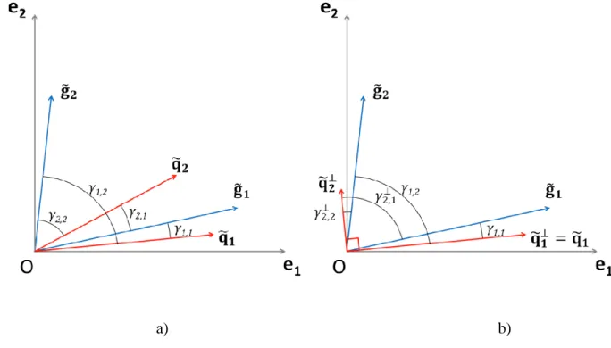
can be described as a vector 𝐠𝑖 (see Figure 1.Erreur ! Source du renvoi introuvable.a.). 138
However, each component 𝑥 of such an LCI result vector, so the elementary flows 𝑔𝑥,𝑖 that form
139
𝐠𝑖, has its own accounting unit (e.g. kilogram, Becquerel, joule...), and within this vector space,
140
no consistent inner product (which induces a norm) can be defined (Heijungs and Suh, 2002). In 141
this perspective, it is useful to recall that the vector spaces that are usually employed in the 142
engineering disciplines refer to 3-dimensional Euclidean space, in which vectors have a magnitude 143
and a direction, and concepts such as angle and distance make sense. In non-metric vector spaces, 144
vectors are more abstractly considered to be 𝑛-tuples, for which such concepts are not defined 145
(Gentle, 2007). In order to be able to measure distances or angles between vectors, we here extend 146
the studied vector space with an inner product after a standardization step. 147
Among the diversity of possible standardizations (min-max, z-score…), the geometric mean of 148
each elementary flow over all products is used in the present work for two reasons. First, the 149
Version postprint
geometric mean is robust to extreme values. Secondly and more importantly, this choice allows 150
our approach being free of the reference flow values of LCI results (i.e. the issue emphasised by 151
Heijungs (2017) about Steinmann et al. (2017) approach; see the section 2.1.2. and SI A.1 for 152
details). Defining 𝐺x as the geometric mean of the 𝑥th elementary flow, so
153 𝐺𝑥= exp ( 1 𝑚 ∑ ln|𝑔𝑥,𝑖| 𝑚 𝑖=1 ) (1)
the 𝑥th standardized elementary flows 𝐠̃
𝑥,𝑖 of the 𝑖th LCI result is:
154
𝑔̃𝑥,𝑖=
𝑔𝑥,𝑖
𝐺𝑥 (2)
Note that we used the absolute value in equation 1 to allow for cases where the values are negative. 155
Within this standardized vector space and given two LCI result vectors 𝐠̃1 and 𝐠̃2, we can define 156
the inner product of these vectors as: 157
〈𝐠̃1, 𝐠̃𝟐〉 = ∑ 𝑔̃𝑥,1𝑔̃𝑥,2 𝑛
𝑥=1
(3)
Next, we define the norm or Euclidean length of a vector 𝐠̃𝑖 as
158
‖𝐠̃𝑖‖ = √〈𝐠̃𝑖, 𝐠̃𝑖〉 (4)
Finally, this allows us to define the angle 𝛼 between two LCI vectors, say, 𝐠̃1 and 𝐠̃2, indicated by 159 𝛼1,2, as 160 𝛼1,2= arccos ( 〈𝐠̃1, 𝐠̃2〉 ‖𝐠̃1‖‖𝐠̃2‖) (5)
Within the standardized vector space, the LCI result of each product has then its own vector 161
direction and norm (see Figure 1.a.). 162
Version postprint
The norm of a standardized LCI result vector still depends on the magnitude of the reference flow 163
of the product, while the direction of the vector doesn’t. This justifies the proposed definition based 164
on the angle between vectors (see part 2.1.2). 165
Regarding impact categories, the consequences of unit amounts of the different elementary flows 166
are summarised by their characterization factors (CFs), the numbers 𝑞𝑥,𝑗. CFs are conversion
167
factors used to assess the elementary flows in terms of impact category results. The collection of 168
CFs of one impact category therefore defines a vector within the elementary flow vector space 169
(according to the Fréchet-Riesz theorem, see Esnouf et al. (2018) section 2.1.2). Figure 1.a. 170
illustrates this for two impact categories, where the vector of CFs is denoted as 𝐪̃1 and 𝐪̃2, after 171
standardization (see below). 172
Because we work with standardized elementary flows, the CFs should be standardized as well to 173
maintain unit consistency: 174
𝑞̃𝑥,𝑗= 𝑞𝑥,𝑗𝐺𝑥 (6)
In this way, by standardizing the impact categories, we can depict the vectors 𝐪̃𝑗 into the same 175
standardized vector space. It reveals the main dimensions that contribute to each of the modelled 176
environmental issues. 177
The LCIA step of the LCA framework translates the LCI result 𝐠𝑖 into a quantified LCIA result 178
ℎ𝑗,𝑖. The scalar ℎ𝑗,𝑖 is the amount of impacts on the 𝑗th impact category for the 𝑖th product using a
179 linear transformation: 180 ℎ𝑗,𝑖= ∑ 𝑞𝑥,𝑗𝑔𝑥,𝑖 𝑛 𝑥=1 (7)
Version postprint
The LCIA result of a standardized LCI result vector 𝐠̃𝑖 with a standardized impact category 𝐪̃𝑗 181
equals to the previous LCIA result ℎ𝑗,𝑖 of the unstandardized vectors: 182 ℎ̃𝑗,𝑖= 〈𝐪̃𝑗, 𝐠̃𝒊〉 = ∑ 𝑞𝑥,𝑗𝐺𝑥 𝑔𝑥,𝑖 𝐺𝑥 𝑛 𝑥=1 = ℎ𝑗,𝑖 (8)
We extend the definition of the inner product of two standardized LCI vectors, say, 〈𝐠̃1, 𝐠̃2〉 to the 183
inner product of two standardized impact categories, say, 〈𝐪̃1, 𝐪̃2〉, and to the inner product of a 184
standardized LCI vector and a standardized impact category 〈𝐪̃𝑗, 𝐠̃𝑖〉 (previously used in equation
185
8 for the definition of the LCIA result ℎ̃𝑗,𝑖). This also allows us to define the norm of an impact 186
category, ‖𝐪̃𝑗‖, the angle between two impact categories, 𝛽, and the angle (𝛾𝑗,𝑖) between an LCI
187
vector 𝐠̃𝑖 and an impact category vector, 𝐪̃𝑗. This finally allows us to define the representativeness 188
index RI between an LCI vector and an impact category, as discussed in the next section. 189
2.1.2. RI between a LCI result and an impact category 190
Within a standardized vector space, the representativeness index (RI) proposed by Esnouf et al. 191
(2018) is a measure between a standardized LCI result (𝐠̃𝑖) vector and an impact category vector 192
(𝐪̃𝑗). In order to be free of the norm of the different vectors, it is based on the angle 𝛾𝑗,𝑖 between
193
an LCI result vector and an impact category vector. The RI of an LCI result 𝐠̃𝑖 for the impact
194 category 𝐪̃𝑗 is: 195 𝑅𝐼𝑗,𝑖 = 𝑅𝐼(𝐪̃𝑗, 𝐠̃𝑖) = |cos(𝛾𝑗,𝑖)| = | 〈𝐪̃𝑗, 𝐠̃𝑖〉 ‖𝐪̃𝑗‖‖𝐠̃𝑖‖ | = | 𝐡𝑗,𝑖 ‖𝐪̃𝑗‖‖𝐠̃𝑖‖ | (9)
The higher the values of the RI, the better the impact category represents the main dimensions of 196
the LCI result vector (i.e. the direction), relatively to the cumulated LCI database. Within the 197
Version postprint
standardized vector space, the representativeness index can then be interpreted as a measure of 198
similarity between the standardized LCI result vector and the standardized impact category vector. 199
200
a) b)
201
Figure 1. a) Representation of two standardized LCI result vectors 𝐠̃𝟏 and 𝐠̃𝟐 (in blue), two 202
standardized impact category vectors 𝐪̃𝟏 and 𝐪̃𝟐 (in red), and the four of the angles 𝜸𝒋,𝒊 used to
203
measure RIs. The vector space is spanned by two basis vectors (𝐞𝟏 and 𝐞𝟐) representing 204
standardized elementary flows, such as CO2 and NOx. b) Illustration of the correlation issue and
205 𝐪
̃𝟐⊥, the orthogonal version of 𝐪̃𝟐 (see below). 206
2.1.3. RI between a LCI result and a LCIA method 207
In addition to the RI between an LCI result and an impact category, we define the RI between an 208
LCI result and an entire LCIA method consisting of a collection of impact categories. An LCIA 209
method can be regarded as a sub-space of the standardized vector generated by the impact 210
Version postprint
categories. The LCIA method is written as a matrix 𝐐, consisting of the 𝑝 different impact 211
categories that belong to that method: 212
𝐐 = (𝐪1 ⋯ 𝐪𝑝) (10)
Because we decided to work in standardized space, we effectively work with 213
𝐐̃ = (𝐪̃1 ⋯ 𝐪̃𝑝) (11)
The RI of the entire LCIA method is then defined, for LCI result 𝐠𝑖, as
214 𝑅𝐼𝑖 = 𝑅𝐼(𝐐̃,𝐠̃𝑖)= √∑(𝑅𝐼(𝐪̃j,𝐠̃𝑖)) 2 𝑝 𝑗=1 (12)
2.1.4 Correlation and decorrelation 215
The impact category vectors of the LCIA method are in general not orthogonal, that is, the angle 216
𝛽 between some of the (standardized) impact category vectors is not 90 degrees. This also implies 217
that for an LCIA method, subsets of non-orthogonal impact category vectors can be observed for 218
which the impact category vectors are correlated with each other. The effect of this is an over- or 219
under-representation of the LCI result vector by those impact category vectors. It relies on the fact 220
that RIs of the non-orthogonal impact category vectors for the LCI result vector will assess and 221
represent the LCI result vector through the same main elementary flows. Indeed, the main direction 222
of a LCI result vector can be close to the main direction of two (or more) non-orthogonal impact 223
category vectors, which lead to an over-representation, or at the opposite, both impact category 224
vectors miss this main direction even if their characterization factors are not null on the main 225
dimensions of the LCI result vector, which then lead to an under-representation. At the LCIA 226
Version postprint
method level, this over or under-representation can be solved by an orthogonalization procedure 227
of the impact category vectors 𝐪̃𝑗 (Esnouf et al., 2018). This procedure is based on the well-known 228
Gram-Schmidt process (Arfken and Weber, 2012). The Gram-Schmidt process returns a new set 229
of standardized perpendicular vectors, which will be denoted here as 𝐪̃𝑗⊥ (see Figure 1.b.). Similar 230
to equation 11, we can pack these vectors for the entire LCIA method in one matrix, 𝐐̃⊥. Using 231
the angle 𝛾𝑗,𝑖⊥ between an LCI result vector 𝐠̃𝑖 and an orthogonalized impact category vector 𝐪̃𝑗⊥,
232
this in turn can serve to calculate a new RI of a LCIA method, similar to equations 9 and 12: 233 𝑅𝐼𝑗,𝑖⊥ = 𝑅𝐼(𝐪̃𝑗 ⊥ ,𝐠̃𝑖)= |cos(𝛾𝑗,𝑖⊥)| (13) and 234 𝑅𝐼𝑖⊥= 𝑅𝐼(𝐐̃⊥,𝐠̃ 𝑖)= √∑(𝑅𝐼𝑗,𝑖⊥) 2 𝑝 𝑗=1 (14)
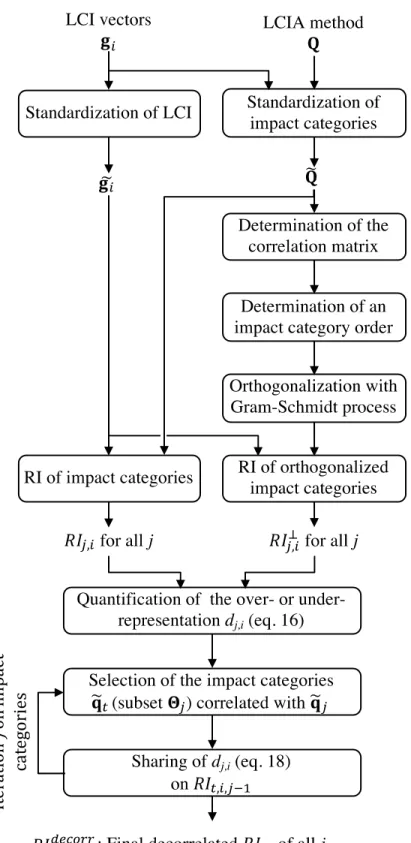
The procedure that is proposed to take into account the over or under-representation for the RIs of 235
impact category belonging to the same LCIA method is schematized in Figure 2. The upper part 236
describes the steps that are needed to obtain 𝑅𝐼𝑖 and 𝑅𝐼𝑖⊥ that are needed to take out the 237
consequences of the correlations between impact category vectors. The lower part describes the 238
iterative loop developed in section 2.1.5. that is needed to solve the consequences triggered by the 239
order dependency of the impact category that is inherent in the Gram-Schmidt process. 240
Version postprint
241
Figure 2. Schematics of the proposed algorithm
Version postprint
The Gram-Schmidt process allows obtaining a set of orthogonal impact category vectors from one 243
LCIA method and thus allows determining its 𝑅𝐼𝑖⊥. But the order of processing the different 𝐪̃𝑗 244
vectors in 𝐐̃ determines the RIs of the standardized and orthogonalized vectors. With the Gram-245
Schmidt iterative process, the first treated vector is not modified (and its RIs will not be different 246
between 𝐪̃1 and 𝐪̃1⊥) while the next vectors are orthogonalized paying regard to the previously
247
handled vectors (and there will be differences between the RIs of 𝐪̃𝑗 and 𝐪̃𝑗⊥ (for 𝑗 = 2, … , 𝑝)).
248
Because of that, the orthogonalized impact category vectors that result from the Gram-Schmidt 249
process cannot be directly used to look at the RIs of 𝐠̃𝑖 for uncorrelated impacts due to this order 250
dependency. 251
To solve the problem of order-dependency we define a unique order of treatment of the impact 252
categories. Instead of applying Gram-Schmidt to the usual order 𝑗 = 1, … , 𝑝, we first sort the 253
impact category vectors, and apply the Gram-Schmidt process to the vectors arranged in that new 254
order. This order is determined by using the correlation matrix of the impact category vectors 255
belonging to 𝐐̃ (see Figure 2). This makes sense because the correlation coefficient of two vectors 256
is equivalent to the cosine of the angle between these vectors (Gniazdowski, 2013), which in turn
257
is equal to the RI as defined above. For each impact category, the sum of the squares of all its 258
correlation coefficients (𝑆𝑆𝑅) is calculated: 259 𝑆𝑆𝑅𝑗= ∑ (𝑟(𝐪̃𝑗, 𝐪̃𝑙)) 2 𝑝 𝑙=1 (15)
This includes the trivial case 𝑙 = 𝑗, for which 𝑟 = 1, but because it doesn’t affect the ranking we 260
can leave it in. The order of impact categories is determined by ranking these sums 𝑆𝑆𝑅𝑗 in 261
Version postprint
descending order. The first impact category to be processed is then the one which has the highest 262
𝑆𝑆𝑅, and the maximal correlation with the other impact categories. 263
The over- or under-representation of an LCI result vector by a set of impact category vectors 264
corresponds to the difference between the RIs measured by the non-orthogonal impact categories 265
and the RIs measured by the orthogonalized impact categories. Based on the determination of those 266
differences, a decorrelation algorithm is proposed in the next section. This algorithm allows 267
distributing the over- or under-representation between the non-orthogonal impact categories 268
(iteration loop in Figure 2). 269
2.1.5. Decorrelation algorithm of impact category RIs 270
From the 𝑅𝐼𝑗,𝑖⊥ determined for a LCIA method after the Gram-Schmidt process, the over- or
under-271
representation need to be quantified and distributed over the subset of non-orthogonal impact 272
categories. For the LCI vector 𝐠̃𝑖 and the impact category 𝐪̃𝑗, the RI of the orthogonalized impacts 273
(𝑅𝐼𝑗,𝑖⊥) is compared to the original one (𝑅𝐼j,i). Their distance 𝑑𝑗,𝑖 (as defined in equation 14) is
274
interpreted as the over- or under-representation of 𝐠̃𝑖 expressed by the impact category 𝑗 and that 275
is redundant or missing regarding the categories that have been previously processed given the 276
order of the impact categories used in the Gram-Schmidt process: 277
𝑑𝑗,𝑖= √(𝑅𝐼𝑗,𝑖) 2
− (𝑅𝐼𝑗,𝑖⊥)2 (16)
The over- or under-representation 𝑑𝑗,𝑖 of the impact category 𝐪̃𝑗 has to be distributed over the other 278
non-orthogonal impact categories. For this purpose, each 𝑑𝑗,𝑖 is treated iteratively with the same 279
order that is used for impact categories in the Gram-Schmidt process. Let Θ𝑗 be the subset of the
Version postprint
category vectors 𝐪̃𝑡 that are correlated to 𝐪̃𝑗, Θ𝑗 = {𝐪̃𝑡|𝑡 ∈ {1, … , 𝑝}, 𝑟(𝐪̃𝑡, 𝐪̃𝑗) ≠ 0}. 𝑅𝐼𝑡,𝑖,𝑗 is the
281
RIs modified by the decorrelation process of the LCI result vector 𝐠̃𝑖 for the impact category 𝐪̃𝑡 282
during the 𝑗th iteration. For the first impact category treated 𝑑
1,𝑖 = 0 (𝑅𝐼1,𝑖⊥ is equal to 𝑅𝐼1,𝑖 because
283 𝐪
̃1 is not modified by the Gram-Schmidt process, so 𝐪̃1⊥ = 𝐪̃1). Consequently, the results 𝑅𝐼𝑡,𝑖,1 of
284
𝐠̃𝑖 for these categories 𝐪̃𝑡 are the original RIs that are obtained from equation 9: 285
𝑅𝐼𝑡,𝑖,1= 𝑅𝐼𝑡,𝑖 (17)
Let 𝑆𝑖 = ∑𝑝𝑡=1(𝑅𝐼𝑡,𝑖,1)2 the sum of the squares of 𝑅𝐼𝑡,𝑖,1. For the following iterations (𝑗 = 2, … , 𝑝), 286
all the 𝑅𝐼𝑡,𝑖,𝑗will share the over or under-representation measured by 𝑑𝑗,𝑖: 287 𝑅𝐼𝑡,𝑖,𝑗= √(𝑅𝐼𝑡,𝑖,𝑗−1) 2 − (𝑑𝑗,𝑖) 2 ×(𝑅𝐼𝑡,𝑖,1) 2 𝑆𝑖 (18)
At the end of the iteration procedure, all the resulting decorrelated RIs, 𝑅𝐼𝑗,𝑖decorr = 𝑅𝐼𝑡,𝑖,𝑝, of 𝐠̃𝑖 288
for the impact category vectors of an LCIA method obtained through this algorithm are free from 289
the consequences of the order of the impact category used within the Gram-Schmidt process. 290
2.2. Material
291
The methodology is applied to the cumulated LCI result version of the ecoinvent 3.1 “allocation 292
at the point of substitution” database (Wernet et al., 2016). This version of the cumulated LCI 293
database was released in 2014. It comprises 11,206 LCI result vectors that are described through 294
1,727 elementary flows (the intervention matrix). The elementary flows vector space therefore has 295
1,727 dimensions. Compared to Esnouf et al. (2018), the same matrix was used although certain 296
elementary flows and LCI results were removed from the cumulated LCI database. Indeed, 297
Version postprint
30 referenced elementary flows are set aside. 142 elementary flows were also not taken into 299
account due to the low number of LCI results that take value on them. 300
The ILCD V1.05 (EC-JRC, 2010a) is the studied LCIA method. It was extracted from the SimaPro 301
8.1.1.16 software to analyse the most recent and operational version. The CF nomenclature was 302
transferred from the SimaPro nomenclature to the ecoinvent elementary flows nomenclature with 303
the assistance of the ecoinvent centre. 304
Implementation was conducted with Python 2.7 on a Jupyter Note-book (Perez and Granger, 2007) 305
(formerly IPython Notebook) and using numerical computation libraries SciPy (V 0.16.0), Pandas 306
(V 0.17.1) and Matplotlib (V 1.5.0). Python is an open-source programming language which is 307
increasingly used in data sciences and in LCA framework as in Brightway2 (Mutel, 2017). 308
An operational tool written with Python 3.6 was also developed. It is available from an online 309
deposit hosted on github.com with the DOI: 10.5281/zenodo.1068914. The package allows to 310
apply the methodology on LCI result excel files (system process) exported from SimaPro and 311
modelled within the ecoinvent 3.1 “allocation at the point of substitution” database (further 312
development needs to be done to apply the methodology to other cumulated LCI databases and to 313
cumulated LCI result files exported from other software). Three outputs can be obtained per LCI 314
result: RIs of LCIA methods, RIs of their impact category vectors and RIs of decorrelated 315
categories. Almost all the multi-criteria LCIA methods can be analysed. Standardization is applied 316
with geometric means of elementary flows after a nomenclature translation from ecoinvent to 317
SimaPro. 318
Based on the studied cumulated LCI ecoinvent database, the LCI results of the Chinese and the 319
German electricity production mixes serve as an illustrative example of the presented work. The 320
Version postprint
two LCI results refer to the market production of 1 kWh of high voltage electricity. The market 321
version of these LCI results models the elementary flows of electricity production mixes, 322
transmission networks and electricity losses during transmission. 323
3. Results and discussion
324
3.1. Illustrative example
325
3.1.1. LCIA results analysis with respect to RIs 326
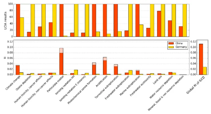
A comparison of LCIA results from the Chinese and the German electricity mixes points to a 327
number of noteworthy elements evidenced by the impact categories RI results (see Figure 3). The 328
upper bar-chart typically illustrates the results of a comparative LCA study, the lower chart 329
represents the outputs of the python package (see data in SI B). For the German mix, ten impact 330
category results are higher than for the Chinese mix, out of the sixteen impact categories of the 331
ILCD method. Germany is two-fold higher for 9 categories: Ozone depletion, Toxicities (cancer 332
and non-cancer effects), Ionizing radiations (human health and ecosystems), Freshwater 333
eutrophication, Ecotoxicity and both Resource depletions. The German mix also uses a higher 334
proportion of land area, but the gap is smaller (China is only 21% lower than Germany on this 335
impact category). Contrasting LCIA results are observed for particulate matter, photochemical 336
ozone formation, acidification and terrestrial eutrophication where China is five times higher than 337
Germany. The same observation can be made for climate change and marine eutrophication but 338
with a lower difference (compared to China, German impacts are lower by 41% and 63% 339
respectively). 340
Version postprint
341
Figure 3. LCIA results (expressed relative to the highest value) and impact category RIs for the
342
LCI results of the Chinese and German electricity mixes from the ILCD method. Bright colours 343
correspond to decorrelated RIs 𝑹𝑰𝒋,𝒊𝐝𝐞𝐜𝐨𝐫𝐫 while pastels colours indicate the part removed from the 344
original RIs by the decorrelation procedure, 𝒅𝒋,𝒊.
345
The global RIs of the ILCD method are 0.113 for the Chinese and 0.0285 for the German mix. The 346
Chinese mix has a better overall representation with this LCIA method because its RI of method 347
is higher. Using impact category RIs from Figure 3, this high overall RI of the method comes from 348
high impact category RI results on particulate matter, acidification, photochemical ozone 349
formation, climate change and terrestrial eutrophication (in decreasing order of contribution). 350
During interpretation, the focus must, in priority, be put on this reduced set of impact category 351
vectors. 352
Version postprint
The main representative impact categories for the German mix are ionizing radiation (HH), 353
freshwater eutrophication, climate change, water resource depletion and human toxicity (non-354
cancer effect). The RIs of these LCIA results are two to three times higher for these impact 355
categories (see Figure 3) and they should be looked at first and foremost for the result 356
interpretation. 357
The environmental issues highlighted for this comparative LCA study are not the same for both 358
LCI results. Given the contextualization of LCI results and impact categories from the cumulated 359
LCI database, the use of 𝑅𝐼𝑗,𝑖 and 𝑅𝐼𝑗,𝑖⊥ guides the LCA practitioner in the interpretation of the main
360
representative impact categories for each LCI result. 361
3.1.2. Example of decorrelation on two LCI results 362
Results from the decorrelation of impact category RI results obtained for the two previously 363
studied LCI results are presented in the Figure 3. Using the 𝑅𝐼𝑗,𝑖 , the equation 12 results in 0.137 364
and 0.0293, respectively for the Chinese and the German mixes, while the overall RIs of the ILCD 365
method are 0.113 and 0.0285 (see above). These differences a dependence between the impact 366
category vectors, which are removed by the presented algorithm. 367
Six impact category RIs are particularly affected by decorrelation (see Figure 3). The algorithm 368
lowers the representativness index of the Chinese mix for the particulate matter, acidification, 369
photochemical ozone formation, and terrestrial eutrophication categories. The climate change and 370
marine eutrophication categories are affected to a lesser extent. The decorrelation of the German 371
mix RIs does not affect its representativeness index on any particular impact category. 372
Orthogonalized results do not modify the previous interpretations. 373
Version postprint
3.2. Global trends of impact category RIs over the cumulated LCI database
374
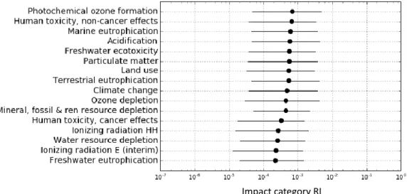
The ordered distribution of the impact category RIs of the entire cumulated LCI database indicates 375
that their values rapidly decrease below 0.1, reaching 10-2 to 10-5 (see Figure 4). These low values 376
result from the high-dimensional vector space in which the study takes place. The ranges of impact 377
category RI values are globally similar when the different impact categories are compared. In an 378
analogous manner, these impact categories represent the different LCI results of the cumulated 379
database, in terms of quantity of information. They all seem relevant for a large number of LCI 380
results. However, all impact categories are probably not compulsory for the analysis of a single 381
LCI result, as observed in the previous illustrative example. 382
383
Figure 4. Range of RI values of the ILCD impact categories regarding the 11206 LCI results of
384
ecoinvent. Shown are: the median (dot), the first quartile (left end of line) and third quartile (right 385
end of line). Impact categories are sorted according to their median. 386
3.3. Decorrelation of impact category RIs within a LCIA method
387
Version postprint
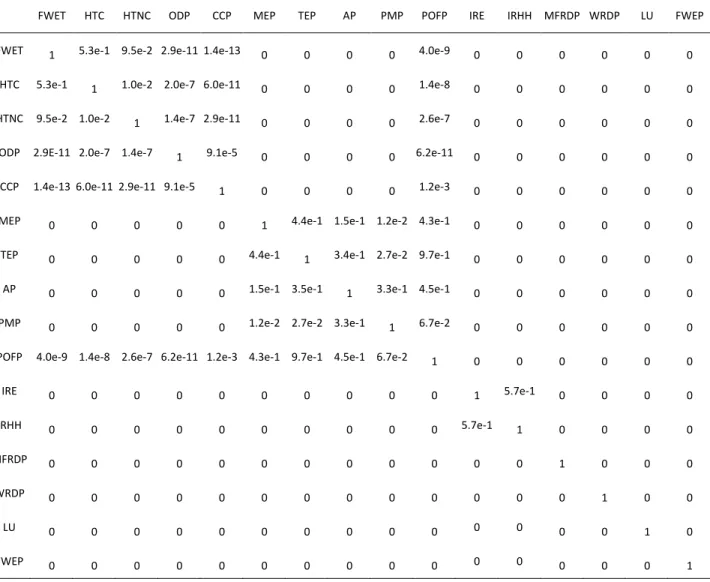
3.3.1. Correlation matrix of impact categories 388
Table 2 presents the correlation matrix of the impact categories (after standardization). Based on 389
their correlation, five different subsets of intercorrelated categories (i.e. Θ𝑗) are labelled from A to 390
E and described in Table 3. Some impact categories feature in two subsets. 391
Table 2. Correlation matrix of impact categories of the ILCD method, on the basis of 11206
392
products from ecoinvent. 393
FWET HTC HTNC ODP CCP MEP TEP AP PMP POFP IRE IRHH MFRDP WRDP LU FWEP FWET 1 5.3e-1 9.5e-2 2.9e-11 1.4e-13 0 0 0 0 4.0e-9 0 0 0 0 0 0
HTC 5.3e-1 1 1.0e-2 2.0e-7 6.0e-11 0 0 0 0 1.4e-8 0 0 0 0 0 0 HTNC 9.5e-2 1.0e-2 1 1.4e-7 2.9e-11 0 0 0 0 2.6e-7 0 0 0 0 0 0 ODP 2.9E-11 2.0e-7 1.4e-7 1 9.1e-5 0 0 0 0 6.2e-11 0 0 0 0 0 0 CCP 1.4e-13 6.0e-11 2.9e-11 9.1e-5 1 0 0 0 0 1.2e-3 0 0 0 0 0 0 MEP 0 0 0 0 0 1 4.4e-1 1.5e-1 1.2e-2 4.3e-1 0 0 0 0 0 0 TEP 0 0 0 0 0 4.4e-1 1 3.4e-1 2.7e-2 9.7e-1 0 0 0 0 0 0 AP 0 0 0 0 0 1.5e-1 3.5e-1 1 3.3e-1 4.5e-1 0 0 0 0 0 0 PMP 0 0 0 0 0 1.2e-2 2.7e-2 3.3e-1 1 6.7e-2 0 0 0 0 0 0 POFP 4.0e-9 1.4e-8 2.6e-7 6.2e-11 1.2e-3 4.3e-1 9.7e-1 4.5e-1 6.7e-2 1 0 0 0 0 0 0 IRE 0 0 0 0 0 0 0 0 0 0 1 5.7e-1 0 0 0 0 IRHH 0 0 0 0 0 0 0 0 0 0 5.7e-1 1 0 0 0 0 MFRDP 0 0 0 0 0 0 0 0 0 0 0 0 1 0 0 0 WRDP 0 0 0 0 0 0 0 0 0 0 0 0 0 1 0 0 LU 0 0 0 0 0 0 0 0 0 0 0 0 0 0 1 0 FWEP 0 0 0 0 0 0 0 0 0 0 0 0 0 0 0 1 394
Table 3. Definition of subsets of impact categories and their abbreviations.
Version postprint
Impact category Abbreviation
Member of subset
A B C D E
Freshwater ecotoxicity FWET X X Human toxicity, cancer
effects HTC X X
Human toxicity,
non-cancer effects HTNC X X
Ozone depletion ODP X X
Climate change CCP X X
Marine eutrophication MEP X X Terrestrial eutrophication TEP X X Acidification AP X X Particulate matter PMP X X Photochemical ozone formation POFP X X X
IRE Ionizing radiation E
(interim) IRE X
Ionizing radiation HH IRHH X
Mineral, fossil & renewable resource depletion MFRDP X Water resource depletion WRDP X Land use LU X Freshwater eutrophication FWEP X 396
The Photochemical ozone formation (within subset C) has a particular position because it 397
correlates with the two subsets A and B which do not have any elementary flows in common. This 398
category is the one with the highest SSR (eq. 15) and is therefore the first one to be processed by 399
the algorithm. Consequently, the orthogonalization of one subset A or B does not affect the 400
orthogonalized RI of the other subsets through Photochemical ozone formation relationships. 401
However, the Photochemical ozone formation is affected by both subset A and B. 402
Version postprint
The two ionizing radiation impact categories (subset D) are only correlated with each other. Impact 403
categories that do not correlate with any other are gathered in subset E. 404
The correlation coefficients point out that subsets B and D present very high correlations (between 405
1.17 × 10⁻² and 4.44 × 10⁻¹) in comparison to subset A (from 1.40 × 10⁻¹³ to 5.32 × 10⁻¹).
406
The Photochemical ozone formation potential also presents higher correlation coefficients with 407
subset B (up to 9.66 × 10⁻¹) than with subset A (up to 1.24 × 10⁻³). 408
3.3.2. Consequences of decorrelation over the cumulated LCI database 409
Orthogonalized impact category RI values are obtained by applying the algorithm to all 11206 410
ecoinvent LCI results. To determine the global trends of the redistribution of the representativeness 411
of impact categories for all LCI results, the distribution of the ratio 𝑅𝐼
decorr−𝑅𝐼
𝑅𝐼 are analysed for
412
each impact category; see Figure 5. Distributions of the ratio are based on the original RI values 413
and the orthogonalized RI values of the impact categories (see equations 16 and 18). For one LCI 414
result, all the RIs of the impacts categories with a similar belonging to the subsets obtain the same 415
ratio (while each LCI result is associated to a unique ratio). That means with the ILCD method 416
that five group are done: Impact categories only in subset A, only in subset B, in A, B and C (i.e. 417
the Photochemical ozone formation category), in D and in E. 418
Version postprint
420
421
Figure 5. Analyses of the different redistribution of RI values. Ordinate refers to the belonging of
422
the impact categories. Shown are: the median (large dot), the first quartile (left end of line), the 423
third quartile (right end of line), and the 5% and 95% percentiles (small dots). 424
Results imply that the major part of the redistribution slightly decreases the RI values from 𝑅𝐼𝑗,𝑖 to 425
𝑅𝐼𝑗,𝑖decorr (between 0 and 20%). Obviously, impact categories that do not correlate with any other 426
impact category do not show any change (subset E). 427
For subsets A, B and C, a decrease is the main tendency but high increases are observed for some 428
inventories, with a 95% percentiles up to 80% (reaching 300% for extreme values). High values 429
are correlated between the impact categories of these 3 subsets (see SI.A.2). However, for the 430
major part of the impact category RIs (negative modifications down to 20%), the correlation 431
appears to be less obvious. Nevertheless, the modifications remain low for each subset. The wide 432
RI redistribution of the photochemical ozone formation (first impact category treated by the 433
algorithm) is triggered by the orthogonalization from the other two subsets that form another 434 “profile” on Figure 5. 435 Subset A only Subset B only Subset A, B & C Subset D Subset E
Version postprint
As for subset D, the distribution of the modifications in impact category RI is very restricted. This 436
could be explained by the fact that only two impact categories belong to this subset. No correlation 437
of the redistribution with the other subsets is observed (see SI A.2). 438
The increase of RI values for 𝑅𝐼𝑗,𝑖decorr is triggered by the high 𝑅𝐼𝑗,𝑖⊥ which is observed for several 439
subsets. A LCI result with an high value on an elementary flow, which is not associated to a high 440
CF of any impact categories, can be highlighted by the orthogonalization step and thus lead to an 441
increase in the RI value. The orthogonalization of the impact category redirects the vector towards 442
a secondary elementary flow (see Figure 1.b). When LCI results have a high value on this second 443
elementary flow, their 𝑅𝐼𝑗,𝑖⊥ tend to increase compared to 𝑅𝐼𝑗,𝑖. Most of the LCI results characterized 444
by higher 𝑅𝐼𝑗,𝑖⊥ originate from agricultural production. This is mainly related to ammonia and nitrate 445
elementary flows. The redistribution of extra information from the secondary elementary flow 446
should provide the impact categories of the subset with an increase that finally allows their 447
𝑅𝐼𝑗,𝑖decorr to comply with the RI of the LCIA method. 448
4. Conclusions
449
This work completes the RI methodology previously developed (Esnouf et al., 2018) by focusing 450
on the appropriateness of impact categories. We propose a freely downloadable operational tool 451
for RI calculation and have applied this methodology to an illustrative example. The impact 452
category RIs have proven that interpretations of LCIA results can be deepened. They can assist 453
practitioners by orientating their analysis towards relevant impact categories. Analyses were also 454
carried out over all LCI results of the cumulated LCI database to extract global RI trends. The 455
same approach could also be used for other ecoinvent versions, cumulated LCI databases or 456
Version postprint
specific fields of activity. Moreover, the cumulated LCI database trends were used here to 457
standardize the impact categories. Other types of standardization, for example, based on the global 458
elementary flows of a geographical area or economic sector, could relate the RI methodology. 459
Finally, a focus on the standardized elementary flows that provide the value of the impact category 460
RIs for each LCI result could be interesting to trace the main directions that are linked to each 461
impact category. 462
An algorithm proposing a solution for correlation issues was developed and implemented within 463
the operational tool. Redundant information was spread out according to the original impact 464
category RI. Further work could focus on other types of algorithms where the whole impact 465
category subset would not be affected by the modification of RIs. Only the impact categories with 466
elementary flows affected by orthogonalization would be affected. Based on the RI methodology 467
and taking into account the consistency of impact categories, relevant impact categories could also 468
derive from different LCIA methods, thus enabling the development of composite LCIA methods. 469
470
SUPPLEMENTARY INFORMATION AND DATA 471
Supplementary Information A. Additional details for the standardization process and scatter matrix 472
of the ratio (𝑅𝐼
decorr−𝑅𝐼)
𝑅𝐼 for the different group of impact categories.
473
Supplementary Information B. An excel file that presents an output example of the Chinese and 474
German LCI result obtained with the python tool-box V. 475
476
CONFLICT OF INTEREST 477
Version postprint
The authors declare no conflict of interest. 478
479
ACKNOWLEDGMENT 480
The authors acknowledge the ecoinvent centre for help provided on database description and data-481 pretreatment. 482 483 FUNDING 484
This work was supported by the Clean, Secure and Efficient Energy societal challenge of the 485
French National Research Agency, under contract GreenAlgOhol ANR-14-CE05-0043. 486
487
REFERENCES 488
Arfken, G.B., Weber, H.J., 2012. Mathematical Methods for Physicists. Academic Press. 489
Bare, J., 2011. TRACI 2.0: the tool for the reduction and assessment of chemical and other 490
environmental impacts 2.0. Clean Technol. Environ. Policy 13, 687–696. 491
https://doi.org/10.1007/s10098-010-0338-9 492
Basson, L., Petrie, J.G., 2007. An integrated approach for the consideration of uncertainty in 493
decision making supported by Life Cycle Assessment. Environ. Model. Softw. 22, 167–176. 494
https://doi.org/10.1016/j.envsoft.2005.07.026 495
Bava, L., Sandrucci, A., Zucali, M., Guerci, M., Tamburini, A., 2014. How can farming 496
intensification affect the environmental impact of milk production? J. Dairy Sci. 97, 4579– 497
Version postprint
93. https://doi.org/10.3168/jds.2013-7530 498
Chen, X., Samson, E., Tocqueville, A., Aubin, J., 2015. Environmental assessment of trout farming 499
in France by life cycle assessment : using bootstrapped principal component analysis to better 500
de fi ne system classi fi cation. J. Clean. Prod. 87, 87–95. 501
https://doi.org/10.1016/j.jclepro.2014.09.021 502
De Saxcé, M., Rabenasolo, B., Perwuelz, A., 2014. Assessment and improvement of the 503
appropriateness of an LCI data set on a system level - Application to textile manufacturing. 504
Int. J. Life Cycle Assess. 19, 950–961. https://doi.org/10.1007/s11367-013-0679-9 505
EC-JRC, 2010a. International Reference Life Cycle Data System (ILCD) Handbook: General 506
guide for Life Cycle Assessment - Detailed guidance, First Edit. ed, European Commission. 507
Institute for Environment and Sustainability. https://doi.org/10.2788/38479 508
EC-JRC, 2010b. International Reference Life Cycle Data System (ILCD) Handbook: Analysing 509
of existing Environmental Impact Assessment methodologies for use in Life Cycle 510
Assessment, First Edit. ed, European Commission. Institute for Environment and 511
Sustainability. 512
Esnouf, A., Latrille, É., Steyer, J.-P., Helias, A., 2018. Representativeness of environmental impact 513
assessment methods regarding Life Cycle Inventories. Sci. Total Environ. 621, 1264–1271. 514
https://doi.org/10.1016/j.scitotenv.2017.10.102 515
Gentle, J.E., 2007. Matrix Algebra, Springer Texts in Statistics. Springer New York, New York, 516
NY. https://doi.org/10.1007/978-0-387-70873-7 517
Gniazdowski, Z., 2013. Geometric interpretation of a correlation. Zesz. Nauk. Warsz. Wyższej 518
Version postprint
Szk. Inform. 7, 27–35. 519
Goedkoop, M., Heijungs, R., Huijbregts, M., Schryver, A. De, Struijs, J., Zelm, R. Van, 2009. 520
ReCiPe 2008: A life cycle impact assessment method which comprises harmonised category 521
indicators at the midpoint and the endpoint level. https://doi.org/10.029/2003JD004283 522
Hauschild, M.Z., Goedkoop, M., Guinée, J., Heijungs, R., Huijbregts, M., Jolliet, O., Margni, M., 523
De Schryver, A., Humbert, S., Laurent, A., Sala, S., Pant, R., 2013. Identifying best existing 524
practice for characterization modeling in life cycle impact assessment. Int. J. Life Cycle 525
Assess. 18, 683–697. https://doi.org/10.1007/s11367-012-0489-5 526
Heijungs, R., 2017. Comment on “Resource Footprints are Good Proxies of Environmental 527
Damage.” Environ. Sci. Technol. 51, 13054–13055. https://doi.org/10.1021/acs.est.7b04253 528
Heijungs, R., Suh, S., 2002. The Computational Structure of Life Cycle Assessment. Eco-529
Efficiency in Industry and Science, Vol. 11. Kluwer Academic Publishers. 530
Huijbregts, M.A.J., Rombouts, L.J.A., Hellweg, S., Frischknecht, R., Hendriks, A.J., van de 531
Meent, D., Ragas, A.M.J., Reijnders, L., Struijs, J., 2006. Is Cumulative Fossil Energy 532
Demand a Useful Indicator for the Environmental Performance of Products ? 40, 641–648. 533
https://doi.org/10.1021/es051689g 534
ISO, 2006. ISO 14044: Environmental Management - Life Cycle Assessment Requirements and 535
Guidelines. Geneva, Switzerland. 536
Lautier, A., Rosenbaum, R.K., Margni, M., Bare, J., Roy, P.-O., Deschênes, L., 2010. 537
Development of normalization factors for Canada and the United States and comparison with 538
European factors. Sci. Total Environ. 409, 33–42. 539
Version postprint
https://doi.org/10.1016/j.scitotenv.2010.09.016 540
Mendoza Beltran, A., Prado, V., Font Vivanco, D., Henriksson, P.J.G., Guinée, J.B., Heijungs, R., 541
2018. Quantified Uncertainties in Comparative Life Cycle Assessment: What Can Be 542
Concluded? Environ. Sci. Technol. acs.est.7b06365. https://doi.org/10.1021/acs.est.7b06365 543
Mouron, P., Nemecek, T., Scholz, R.W., Weber, O., 2006. Management influence on 544
environmental impacts in an apple production system on Swiss fruit farms: Combining life 545
cycle assessment with statistical risk assessment. Agric. Ecosyst. Environ. 114, 311–322. 546
https://doi.org/10.1016/j.agee.2005.11.020 547
Mutel, C., 2017. Brightway: An open source framework for Life Cycle Assessment. J. Open 548
Source Softw. 2, 236. https://doi.org/10.21105/joss.00236 549
Pascual-González, J., Guillén-Gosálbez, G., Mateo-Sanz, J.M., Jiménez-Esteller, L., 2016. 550
Statistical analysis of the ecoinvent database to uncover relationships between life cycle 551
impact assessment metrics. J. Clean. Prod. 112, 359–368. 552
https://doi.org/10.1016/j.jclepro.2015.05.129 553
Pascual-González, J., Pozo, C., Guillén-Gosálbez, G., Jiménez-Esteller, L., 2015. Combined use 554
of MILP and multi-linear regression to simplify LCA studies. Comput. Chem. Eng. 82, 34– 555
43. https://doi.org/10.1016/j.compchemeng.2015.06.002 556
Perez, F., Granger, B.E., 2007. IPython: A System for Interactive Scientific Computing. Comput. 557
Sci. Eng. 9, 21–29. https://doi.org/10.1109/MCSE.2007.53 558
Pozo, C., Ruíz-Femenia, R., Caballero, J., Guillén-Gosálbez, G., Jiménez, L., 2012. On the use of 559
Principal Component Analysis for reducing the number of environmental objectives in multi-560
Version postprint
objective optimization: Application to the design of chemical supply chains. Chem. Eng. Sci. 561
69, 146–158. https://doi.org/10.1016/j.ces.2011.10.018 562
Prado-Lopez, V., Seager, T.P., Chester, M., Laurin, L., Bernardo, M., Tylock, S., 2014. Stochastic 563
multi-attribute analysis (SMAA) as an interpretation method for comparative life-cycle 564
assessment (LCA). Int. J. Life Cycle Assess. 19, 405–416. https://doi.org/10.1007/s11367-565
013-0641-x 566
Steinmann, Z.J.N., Schipper, A.M., Hauck, M., Giljum, S., Wernet, G., Huijbregts, M.A.J., 2017. 567
Resource Footprints are Good Proxies of Environmental Damage. Environ. Sci. Technol. 51, 568
6360–6366. https://doi.org/10.1021/acs.est.7b00698 569
Steinmann, Z.J.N., Schipper, A.M., Hauck, M., Huijbregts, M.A.J., 2016. How Many 570
Environmental Impact Indicators Are Needed in the Evaluation of Product Life Cycles? 571
Environ. Sci. Technol. 50, 3913–3919. https://doi.org/10.1021/acs.est.5b05179 572
Téno, J.-F. Le, 1999. Visual data analysis and decision support methods for non-deterministic 573
LCA. Int. J. Life Cycle Assess. 4, 41–47. https://doi.org/10.1007/BF02979394 574
Wernet, G., Bauer, C., Steubing, B., Reinhard, J., Moreno-Ruiz, E., Weidema, B., 2016. The 575
ecoinvent database version 3 (part I): overview and methodology. Int. J. Life Cycle Assess. 576
21, 1218–1230. https://doi.org/10.1007/s11367-016-1087-8 577
578