HAL Id: hal-01019431
https://hal.archives-ouvertes.fr/hal-01019431
Submitted on 7 Jul 2014
HAL is a multi-disciplinary open access
archive for the deposit and dissemination of
sci-entific research documents, whether they are
pub-lished or not. The documents may come from
teaching and research institutions in France or
abroad, or from public or private research centers.
L’archive ouverte pluridisciplinaire HAL, est
destinée au dépôt et à la diffusion de documents
scientifiques de niveau recherche, publiés ou non,
émanant des établissements d’enseignement et de
recherche français ou étrangers, des laboratoires
publics ou privés.
High rate-localization for high-speed all-terrain robots
Cyril Roussillon, Simon Lacroix
To cite this version:
Cyril Roussillon, Simon Lacroix. High rate-localization for high-speed all-terrain robots. IEEE 2nd
International Conference on Communications, Computing and Control Applications (CCCA), Sep
2012, Marseille, France. pp.1-8, �10.1109/CCCA.2012.6417929�. �hal-01019431�
High rate-localization for high-speed all-terrain robots
Cyril Roussillon and Simon Lacroix
Abstract— Localization plays a central role in autonomous robot navigation, and a vast number of contributions can be found in the robotics literature. High speed all terrain robots raise new challenges for localization, that must run at higher rates, while being more accurate than for walking speed robots. The article presents a SLAM setup that satisfies these requirements, using vision and low-cost inertial sensors as its core. Other localization sensors can also be incorporated, such as GPS or odometry, yielding a system that estimate the robot pose and velocity parameters at 100 Hz, with translation errors on the pose of the order of 1m for 500m long trajectories.
I. INTRODUCTION
Most field robotics applications would benefit from faster operations, which implies faster robots. Augmenting the speed of all-terrain robots raises several challenges, the main one being the fact that the vehicle dynamics must be considered for both path planning and path tracking pro-cesses, which is all the more difficult with hardly predictable vehicle/ground interactions. Moving at higher speeds also impacts the perception processes: the robot must perceive the terrain further away in order to assess feasible paths, and process the gathered data at a speed compatible with its motions. One of the key to cope with computation limitations, is to exploit approaches that comply with an economy of means principle [1].
But high motion speeds also imply stringent constraints on the rate and precision of the localization processes. Localization is essential to autonomous navigation, and is notably required to ensure (i) the spatial consistency of the terrain model built to plan paths and (ii) the proper tracking of the paths. Both functions require precise pose estimates: for instance, a 1◦ error on the robot pitch angle
yields a 17cm error on the elevation of a point detected at 10.0m, a distance at which precise information on the terrain is required for speeds above a few m/s, and the robot position and heading must be precisely known to track paths at such speeds. Both functions also require a given frequency of the pose estimates. Path tracking does not require very high rate localization (e.g. in [2] a10Hz rate is sufficient to control a robot at8m/s: the response time of the actuators and the robot dynamics are such that a higher rate is not necessary), but terrain modelling processes do require high rate localization. Since every data perceived on the environment must be precisely localized to be incorporated in the model that represents the environment geometry, the robot pose must be known at the exact time data are gathered.
CNRS; LAAS; 7 avenue du colonel Roche, F-31077 Toulouse, France Université de Toulouse ; UPS, INSA, INP, ISAE; LAAS; F-31077 Toulouse, France
The use of rotating Lidar that continuously stream range data are becoming popular in field robotics (for instance the Velodyne Lidar simultaneously fires 64 lasers at about 4kHz): in the absence of “continuous localization”, the produced images are warped because of the robot translations and of the attitude variations, that can not be neglected for all-terrain robots. Finally, locomotion monitoring to detect faults such as slippages may also benefit from precise high rate pose estimates.
SLAM processes have shown to be elegant and robust so-lutions to the localization problem, and the robotics literature now abounds with analyses of the problem, proposals of theoretical solutions and practical setups (see e.g. [4], [5] for a rather complete synthesis). In this paper we present a SLAM solution that estimates the pose and velocities of a robot at 100 Hz, thus making it usable for high speed all-terrain robots. It mainly relies on a low-cost inertial measurement unit (IMU) to predict the robot motions, and on vision to observe landmarks of the environment. These two sensors form the backbone of our approach, according to a classical motion prediction / landmark observation scheme, implemented with an extended Kalman filter. To improve the consistency of the system, and in particular to avoid the scale drift factor inherent to monocular SLAM approaches and that is not perfectly corrected with low cost inertial sensors, direct observations of the robot state provided by other sensors (namely odometry and GPS) are incorporated in the filter.
Our solution relies on RT-SLAM, an open-source software framework originally presented in [6], whose architecture is summarized in section II. Section III depicts the way the images are processed so as to optimize computation time, while ensuring that no outliers are integrated within the filter. Section IV briefly depicts the way the IMU is used to predict the robot motions, and section V introduces how odometry and GPS pose measurements are introduced within the filter for a better robustness and precision over time. Finally section VI depicts some results, and in particular the benefits of using the additional sensors.
II. OVERALLRT-SLAM ARCHITECTURE
RT-SLAM is a generic, efficient and flexible SLAM appli-cations development tool, which is tailored to yield on-board robust and real-time solutions. RT-SLAM stands for “Real-Time SLAM”, and is available as open source software at http://rtslam.openrobots.org.
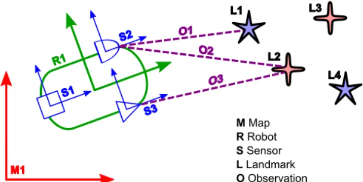
Fig. 1 presents the main objects defined in RT-SLAM. They encompass the basic concepts of a SLAM solution: the world or environment contains maps; maps contain robots and landmarks; robots have sensors; sensors can
make observations of landmarks. Each of these objects is abstract and can have different implementations. They can also contain other objects that may themselves be generic.
R1 S2 S1 S3 M1 L1 L3 L2 L4 O1 O2 O3 M Map R Robot S Sensor L Landmark O Observation
(a) Main objects in a SLAM context. Different robots R have several sensors S, that can provide observations O of landmarks Lmk. States of robots, sensors and landmarks are stored in the stochastic map Map.
(b) Objects hierarchy in RT-SLAM. Each individual map M in the world W contains robots R and landmarks L. A robot has sensors S, and an observation O is created for every pair of sensor and landmark. In order to allow full genericity, map managers MM and data managers DM are introduced.
Fig. 1. The main objects in RT-SLAM
a) Map: The maps contain an optimization or estima-tion engine: for now RT-SLAM uses a standard formulaestima-tion of EKF-SLAM. Since this solution is very well documented in the literature [9], it is not detailed in depth here. Indirect indexing within Boost’s ublas C++ structures is intensively used to exploit the sparsity of the problem and the symmetry of the covariances matrices.
b) Robot: Robots can be of different type according to the way their state is represented and their prediction model. The latter can be either a simple kinematic model (constant velocity, constant acceleration, . . . ) or a proprio-ceptive sensor (odometry, inertial, . . . ), as illustrated section IV. The proprioceptive sensor is an example of generic object contained in robot objects, as different hardware can provide the same function.
c) Sensor: We distinguish two kinds of sensors. The first kind are exteroceptive sensors, that observe landmarks in the environment. Similarly to robots, they can also have different models (perspective camera, panoramic catadioptric
camera, laser, . . . ), and contain a generic exteroceptive sensor hardware object (firewire camera, USB camera, . . . ). The second kind are proprioceptive sensors, that directly observe the pose of the robot and help for localization. Note that this acceptation of the term “proprioceptive” is here quite different from its original meaning in physiology: proprioceptive sensors are the ones that directly observe the state of the robot (or a part of the state), as opposed to exteroceptive sensors that observe the environment. Thus we list as proprioceptive sensors inertial sensors, odometry, GPS, magnetometers, barometers etc, even if some actually observe properties of the environment – accelerometers ob-serve earth gravity, magnetometers obob-serve magnetic field, barometers observe air pressure.
In addition, as sensors belong to the map, their state can be estimated: this opens the possibility for estimating other parameters such as extrinsic calibration, time delays, biases and gain errors, and the like.
d) Landmark: Landmarks can be of different type (points, lines, planes, . . . ), and each type can have different state parametrization (Euclidean point, inverse depth point, . . . ). Moreover the parametrization of a landmark can change over time, as explained section III-B. A landmark also contains a descriptor dedicated to data association, which is a dual description to the state representation.
As shown Fig. 1(a), it is worth noticing that landmark objects are common to the different sensors, all of them being able to observe the same landmark (provided they have com-patible descriptors for this landmark of course). This allows to greatly improve the observability of landmarks compared to a system where the sensors are strictly independent. In the particular case of two cameras for instance, landmarks can be used even if they are only visible from one camera or if they are too far away for a stereovision process to observe their depth (this process was introduced in [10] as BiCam SLAM).
e) Observation: In RT-SLAM, the notion of observa-tion plays a predominant role. An observaobserva-tion is a real object containing both methods and data. One observation is instantiated for every sensor-landmark pair, regardless of the sensor having actually observed the landmark or not, and has the same lifetime as the associated landmark. The methods it contains are the conventional projection and back-projection models (that depend on the associated sensor and landmark models), while the stored data consist of results and intermediary variables such as Jacobian matrices, predicted and observed appearances, innovations, event counters and others, that allow to greatly simplify and optimize computa-tions.
f) Managers: In order to achieve full genericity wrt landmark types, in particular to allow the concurrent use of different landmark types for one sensor, two different manager objects are added: data manager and map manager. Their implementations define a given management strategy, while their instantiations are dedicated to a certain landmark type. The data manager processes the sensors raw data, providing observations of the external landmarks. For this
purpose, it exploits some raw data processors (for feature detection and tracking), and decides which observations are to be corrected and in which order, according to the quantity of information they bring and their quality. For example it can apply an active search strategy and try to eliminate outliers as described in section III-A. The map manager keeps the map clean, with relevant information, and at a manageable size, by removing landmarks according to their quality and the given policy (e.g. visual odometry where landmarks are discarded once they are not observed, or multimap slam where maps are “closed” according to given criteria). These managers communicate together: for example, the data manager may ask the map manager if there is enough space in the map to start a new initialization process, and to allocate the appropriate space for the new landmark.
III. VISUAL PROCESSING WITHINRT-SLAM Vision is currently the only exteroceptive sensor imple-mented in RT-SLAM. The processing of images for a SLAM setup is quite complex, and calls for the definition of several key processes that are summarized here.
A. Active search and one-point RANSAC
The strategy currently implemented in RT-SLAM data manager to deal with observations is an astute combination of active search [9] and outliers rejection using one-point RANSAC [11].
The goal of active search is to minimize the quantity of raw data processing by constraining the search in the area where the landmarks are likely to be found. Observations outside of this 3σ observation uncertainty ellipse would be anyway considered incompatible with the filter and ignored by the gating process. In addition active search gives the possibility to decide anytime to stop matching and updating landmarks with the current available data, thus enabling hard real-timeconstraints. We extended the active search strategy to landmark initialization: each sensor strives to maintain features in its whole field of view using a randomly moving grid of fixed size, and feature detection is limited to empty cells of the grid. Furthermore the good repartition of features in the field of view ensures a better observability of the motions.
Outliers can come from matching errors in raw data or mobile objects in the scene. Gating is not always discrim-inative enough to eliminate them, particularly right after the prediction step when the observation uncertainty ellipses can be quite large – unfortunately at this time the filter is very sensitive to faulty corrections because it can mistakenly make all the following observations incompatible. To prevent faulty observations, outliers are rejected using a one-point RANSAC process. It is a modification of RANSAC, that uses the Kalman filter to obtain a whole model with less points than otherwise needed, and provides a set of strongly compatibleobservations that are then readily corrected. Con-trary to [11] where data association is assumed given when applying the algorithm, we do the data association along
with the one-point RANSAC process: this allows to look for features in the very small strongly compatible area rather than the whole observation uncertainty ellipse, and to save additional time for raw data processing.
B. Landmark parametrization and re-parametrization In order to solve the problem of adding to the EKF a point with unknown distance and whose uncertainty cannot be represented by a Gaussian distribution, point landmarks parametrization and initialization strategies for monocular EKF-SLAM have been well studied [12] [13] [14]. The solutions now widely accepted are undelayed initialization techniques with inverse depth parametrization. Anchored Homogeneous Point [15] parametrization is currently used in RT-SLAM.
The drawback of inverse depth parametrization is that they describe a landmark by at least 6 variables in the stochastic map, compared to only 3 for an Euclidean point (x y z)T. Memory and temporal complexity being quadratic with the map size for EKF, there is a factor of 4 to save in time and memory by reparametrizing landmarks that have converged enough [16]. The map manager uses the linearity criterion proposed in [14] to control this process.
C. Image processing
g) Point extraction: Point extraction is based on Harris detector with several optimizations. Some of them are ap-proximations: a minimal derivative mask [−1, 0, 1] is used, as well as a square and constant convolution mask, in order to minimize operations. This allows the use of integral images [17] to efficiently compute the convolutions. Additional optimizations are related to active search (section III-A): only one new feature is searched in a small region of interest, which eliminates the costly steps of thresholding and sub-maxima suppression.
h) Point matching: Point matching is based on Zero-mean Normalized Cross Correlation (ZNCC), also with several optimizations. Integral images are used to compute means and variances, and a hierarchical search is made (two searches at half and full resolution are sufficient). We also implemented bounded partial correlation [18] in order to interrupt the correlation score computation when there is no more hope to obtain a better score than the threshold or the best one up to now. To be robust to viewpoint changes and to track landmarks longer, tracking is made by comparing the initial appearance of the landmark with its current predicted appearance [9].
IV. MOTION PREDICTION
A. Motion model-based prediction
In the absence of any additional sensor, a motion model is required to predict the state at the time observations are integrated in the filter. A constant velocity model is often used in vision-based SLAM systems. Velocities must then be included in the robot state to be estimated:
where p and q are respectively the position and quaternion orientation of the robot, and v and w are its linear and angular velocities. The predict equation is then:
p+= p+v.dt q+= q∗w.dt v+= v w+= w The covariance matrix is predicted with the Jacobians of the predict equations for p and q, and with the uncertainty of the model for v and w, that represents how much the robot actual dynamic may differ from the model. For a constant velocity model, it is defined by the maximal linear and angular accelerations that the robot can experience.
The advantage of the constant velocity model is its sim-plicity, but it rapidly fails when the system is subject to dynamic motions. A more realistic motion model can be provided by the robot dynamic model parametrized by the applied controlu, but this is hardly feasible with a high speed ground robot, for which the terrain irregularities generate unpredictable perturbations.
B. IMU-based prediction
The pure visual SLAM approach described in the previous section suffers from several drawbacks that can be lessened by using additional sensors:
• The scale factor is not estimated. This can be solved
by using a second camera with a known baseline, or by using a proprioceptive sensor that provides velocity information.
• Search areas for landmark matching in the image can be
large as a kinematic model is not very precise. Using a proprioceptive sensor reduces the landmark uncertainty ellipses and hence speeds up image processing.
• Linearisation points are not very accurate, again as a
consequence of the poor precision of the kinematic model. Using another sensor at a higher rate will allow to exploit the kinematic model at a shorter term where it will be more precise, improving SLAM precision or permitting to reduce the frame-rate to decrease CPU load for equivalent quality.
• Very high motion dynamics are difficult to track
be-cause the uncertainty of the kinematic model has to be increased even more, and the very large uncertainty ellipses implied increase the matching time and the risk of wrong matching.
The use of sensors for the prediction step is computation-ally cheap, as only the covariance matrix part that depends on the robot state is updated, which is significantly smaller than the whole filter state covariance matrix that contains the landmarks. The sensor must nevertheless fulfill the following constraints to be eligible:
1) It is periodic with a higher frequency than any other sensor integrated in the filter,
2) It provides complete data, i.e. that enables to predict all the robot state parameters – otherwise a kinematic or dynamic model is still needed to complete the prediction,
3) It has a reasonably low level of noise, so that it provides a good linearisation point,
4) It is never faulty, i.e. its errors are always consistent with its uncertainty, and it has a Gaussian probability. 5) It does not measure a quantity that is redundant with an other sensor, otherwise it would constantly override its measures instead of being fused with.
An IMU satisfies all these requirements: it is fast and its instantaneous measures are precise, thus yielding predictions around which linearisations do not induce errors. It also stabilizes the attitude angles thanks to the observation of the earth gravity, and it complements well vision in the SLAM problem, as it provides better observability of the scale factor. When using an IMU to predict motions, the robot state becomes:
R= (p q v ab wb g)T
where ab and wb are the accelerometers and gyrometer
biases, andg the norm of the gravity vector. Estimating only the norm of the gravity vector requires a correct initialization of the attitude of the robot, which can easily be done with initial acceleration measures acquired when the robot is static, which is not a strong operational constraint.
A special care has to be taken for the conversion of the noise from continuous time (provided by the manufacturer in the sensor’s datasheet) to discrete time. As the perturbations are continuous white noise, the variance of the discrete noise grows linearly with the integration period.
V. ADDITIONAL OBSERVATIONS
The IMU does not directly measures velocities, but accel-erations that are biased: it can only provide a correct scale factor observation if these biases are properly estimated. Good observability of these biases is a difficult task: it requires the trajectory to stimulate all the degrees of freedom, and the filter must remain consistent in the long term. These conditions are hardly met with a typical robot trajectory, that usually mainly goes forward with limited turns, and because it covers large distances with landmarks that are often renewed, easing a drift of the scale factor estimation. And when the camera loses track of all the landmarks, the scale factor drift biases the new landmarks position estimates, leading the filter to become inconsistent.
A. Odometry
Odometry is an ambivalent sensor: it provides most of the time a precise and stable estimation of the robot velocity, but it can also deliver very faulty data, e.g. when the robot experiences slippages.
There are two common flaws in odometry integration: 1) Using it in the prediction step of the filter. When faulty
measures are not identified as such, observation are not consistent with the prediction and either rejected by a gating process or badly integrated in the filter. 2) Assuming that odometry provides the complete
veloc-ity vector, oriented along the forward axis of the robot. This is wrong whenever the robot is not rigid: because of tires or suspension, the robot body (on which observation sensors are rigidly tied) is not actually
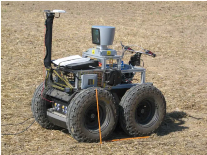
Fig. 2. The robot Mana
moving along the estimated direction. This discrepancy all the more important when the robot is moving at high speeds.
Thus in RT-SLAM odometry is integrated by observing only the normof the robot velocity. This allows to properly estimate the scale factor by providing correct velocities, and to reject faulty data by gating out inconsistent values.
Our robot Mana is built upon a Segway RMP400 plat-form (figure 2), and the odometry provides the independent velocities and torques of the four wheels. This enables to dynamically compute an estimation of the uncertainty of odometry according to the consistency of these measures. For now this estimation is made by analysing the homogeneity of rear and front wheels velocities and torques, and the absolute values of the acceleration, the turn radius and the torques – a machine learning approach to derive this estimation should give better results. However it is important to notice that this uncertainty that takes into account the fault risk can not be used by the gating process, because it would render the faulty data consistent. It is better to use the basic Gaussian uncertainty for the gating, so as to completely reject faulty measures.
Another purpose of odometry integration is to stabilize the system when vision is not working. For instance if the environmental conditions prevent the camera from observing landmarks (masking, low light, sun blinded, etc), then the IMU is not stabilized anymore and quickly starts drifting: odometry help stabilizing the system in such cases. For more efficiency, it is possible to consider again that the odometry observes the complete velocity vector but with higher uncertainty. In particular one can assume that the lateral component of the velocity is usually null, and use gating to detect when it is not the case.
B. GPS
All the sensors described above will not prevent the esti-mation of the robot’s pose to drift on large scale trajectories (except the attitude angles that are stabilized by the IMU). If GPS signal is available, even occasionally, it will not only bound the position error, but also the heading error
by comparing the direction of the local velocity estimated by vision and IMU to the direction of the global velocity provided by the GPS measures (even if GPS provides only position measures).
The easiest way to integrate GPS is known as loose inte-gration, and consists in directly using the position measures computed by the GPS. On the contrary, tight integration uses the raw observations of pseudo-distances to the satellites and reimplements the GPS equations in the filter, which is more precise but also a lot more complex. Thus we only perform loose integration in RT-SLAM.
This naturally works very well with RTK-GPS, because its noise has a Gaussian distribution as required by the filter. However the error of natural GPS is highly biased, mainly by perturbations in the atmosphere that change very slowly. Consequently it must be observed at a limited frequency to avoid being affected too much by this bias.
VI. RESULTS
Videos illustrating the test sequences can be downloaded at http://rtslam.openrobots.org/Material/ CCCA2012. As this sequences taken by our robot Mana cover quite long distances, it is not possible to recall all observed landmarks – otherwise the system would be far from real-time. A solution to this problem is to build several submaps, but as this is not implemented yet in RT-SLAM we are running “short-term SLAM”, immediately forgetting landmarks when they are lost.
A. First sequence
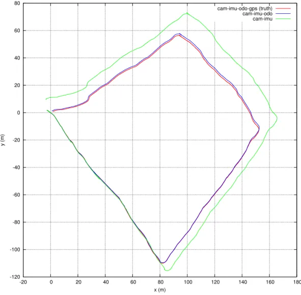
The first sequence represents Mana navigating au-tonomously along a 450m trajectory at 1.5m/s. It is driving half on a road and half on an irregular grassy terrain, reaching successive waypoints while avoiding obstacles thanks to a digital terrain map built from its Velodyne sensor data integrated with our localization (see section VI-C).
Figure 3 shows the trajectory for different combinations of sensors. The trajectory which is using RTK-GPS (with centimetre accuracy at 20Hz) can be considered as ground truth for the position. The trajectory with only camera and IMU illustrates the difficulties it to correctly estimate the scale factor. Adding odometry bounds the position error to a few meters, as shown in more detail figure 4.
B. Second sequence
The second sequence represents Mana navigating au-tonomously at 3m/s, again on grassy and concrete terrains. A this speed our basic control algorithms reach their limits, so the trajectory is quite jerky.
Figures 5 and 6 show two things. First as there are a lot of accelerations and stops, the scale factor is better observed by the system with only camera and IMU. Second, as the robot is constantly turning left and right it renews very often its landmarks, which makes the heading drift faster. That is why there is no significant difference in accuracy with and without odometry.
-120 -100 -80 -60 -40 -20 0 20 40 60 80 -20 0 20 40 60 80 100 120 140 160 180 y (m) x (m) cam-imu-odo-gps (truth) cam-imu-odo cam-imu
Fig. 3. Trajectories estimated on the first sequence with different combinations of sensors
0 0.2 0.4 0.6 0.8 1 1.2 1.4 1.6 0 50 100 150 200 250 300 350 400 Position error (m) Time (s) Position error (m) Height error (m)
-40 -30 -20 -10 0 10 20 30 -60 -50 -40 -30 -20 -10 0 10 y (m) x (m) cam-imu-odo-gps (truth) cam-imu-odo cam-imu
Fig. 5. Trajectories of the robot Mana on the second sequence with different set of sensors
0 0.5 1 1.5 2 2.5 3 3.5 0 20 40 60 80 100 120 140 Position error (m) Time (s) Position error (m) Height error (m)
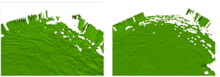
Fig. 7. A digital terrain map of a flat grassy area, built from Velodyne lidar range data using attitude angles provided by an INS (left) and by RT-SLAM (right), while the robot is moving at 2m/s. Erroneous and delayed attitude angles estimates of the INS corrupt significantly the range data, and hinders the building of a precise terrain model.
C. Attitude angles estimation
It is difficult to evaluate the precision of the attitude angle estimation in the absence of ground truth. Nevertheless, the “quality” of the digital terrain model built using range data acquired while to robot is moving provides insights on the precision of RT-SLAM. Figure 7 compares two digital terrain maps built with the Xsens MTi configured as an INS to provide pitch and roll to a 3D odometry localization process, and with RT-SLAM integrating the same Xsens MTi configured as an IMU with camera and odometry.
VII. SUMMARY
We focused in this paper on the fact that high speed and precise localization is necessary for faster autonomous robots, and presented how this can achieved on the basis of vision/INS SLAM approach, complemented by additional proprioceptive sensors for better consistency of the position estimates on the long run. Results show that this 100 Hz localization system allows to build precise terrain models from range data at speeds up to several meter per seconds, and1m accuracy position estimates overs several hundreds meters long trajectories. Higher rates are easily reachable with a faster CPU: RT-SLAM requires a single-core 3GHz processor to process INS data at 100 Hz and VGA images at 50Hz.
REFERENCES
[1] A. Kelly and A. Stentz, “Minimum throughput adaptive perception for high speed mobility,” in International Conference on Intelligent Robots and Systems, Grenoble (France), September 1997, pp. 215–223. [2] R. Lenain, B. Thuilot, and O. H. an P. Martinet, “High-speed mobile
robot control in off-road conditions: a multi-model based adaptive approach,” in IEEE International Conference on Robotics and Au-tomation, Shangaï (China), May 2011.
[3] C. Brenneke, O. Wulf, and B. Wagner, “Using 3d laser range data for slam in outdoor environments,” in International Conference on Intelligent Robots and Systems, 2003, pp. 188–193.
[4] T. Bailey and H. Durrant-Whyte, “Simultaneous Localisation and Mapping (SLAM): Part I The Essential Algorithms,” IEEE Robotics and Automation Magazine, vol. 13, no. 2, pp. 99–110, June 2006. [5] H. Durrant-Whyte and T. Bailey, “Simultaneous Localisation and
Mapping (SLAM): Part II State of the Art,” IEEE Robotics and Automation Magazine, vol. 13, no. 3, pp. 108–117, June 2006. [6] C. Roussillon, A. Gonzalez, J. Solà, , J.-M. Codol, N. Mansard,
S. Lacroix, and M. Devy, “Rt-slam: a generic and real-time slam architecture,” in International Conference on Vision Systems, Sophia Antopolis (France), Sept. 2011.
[7] K. Lingemann, A. Nuchter, J. Hertzberg, and H. Surmann, “High-speed laser localization for mobile robots,” Robotics and Autonomous Systems, vol. 51, no. 4, pp. 275–296, 2005.
[8] P. Gemeiner, A. Davison, and M. Vincze, “Improving localization robustness in monocular SLAM using a high-speed camera,” in Proceedings of Robotics: Science and Systems IV, Zurich, Switzerland, June 2008.
[9] A. Davison, I. Reid, N. Molton, and O. Stasse, “Monoslam: Real-time single camera slam,” IEEE Trans. Pattern Anal. Mach. Intell., vol. 29, pp. 1052–1067, 2007. [Online]. Available: http: //dx.doi.org/10.1109/TPAMI.2007.1049
[10] J. Sola, A. Monin, and M. Devy, “Bicamslam: Two times mono is more than stereo,” in Proc. of IEEE International Conference on Robotics and Automation (ICRA), 2007, pp. 4795 –4800.
[11] J. Civera, O. Grasa, A. Davison, and J. Montiel, “1-point ransac for ekf-based structure from motion,” in Proc. of IEEE/RSJ International Conference on Intelligent Robots and Systems (IROS), oct 2009, pp. 3498 –3504.
[12] A. Davison, “Real-time simultaneous localisation and mapping with a single camera,” in Proc. of IEEE International Conference on Computer Vision (ICCV), oct 2003, pp. 1403–1410. [Online]. Available: http://pubs.doc.ic.ac.uk/single-camera-slam/
[13] T. Lemaire, S. Lacroix, and J. Sola, “A practical 3d bearing-only slam algorithm,” in Proc. of IEEE/RSJ International Conference on Intelligent Robots and Systems (IROS), aug 2005, pp. 2449 – 2454. [14] J. M. M. Montiel, “Unified inverse depth parametrization for
monocu-lar slam,” in Proc. of Robotics: Science and Systems (RSS), 2006, pp. 16–19.
[15] J. Sola, “Consistency of the monocular ekf-slam algorithm for three different landmark parametrizations,” in Proc. of IEEE International Conference on Robotics and Automation (ICRA), may 2010, pp. 3513 –3518.
[16] J. Civera, A. Davison, and J. Montiel, “Inverse Depth to Depth Conversion for Monocular SLAM,” Proc. of IEEE International Conference on Robotics and Automation (ICRA), pp. 2778–2783, apr 2007. [Online]. Available: http://dx.doi.org/10.1109/ROBOT.2007. 363892
[17] P. Viola and M. Jones, “Rapid object detection using a boosted cascade of simple features,” in Proc. IEEE Conf. Comput. Vis. Pattern Recog, 2001, pp. 511–518.
[18] L. D. Stefano, S. Mattoccia, and F. Tombari, “Zncc-based template matching using bounded partial correlation,” Pattern Recognition Letters, vol. 26, no. 14, pp. 2129 – 2134, 2005. [Online]. Available: http://www.sciencedirect.com/science/ article/B6V15-4G3619F-7/2/c051cecd4a8d442e1fa8aa5c228c259c