HAL Id: hal-02147763
https://hal.archives-ouvertes.fr/hal-02147763
Submitted on 5 Jun 2019
HAL is a multi-disciplinary open access
archive for the deposit and dissemination of
sci-entific research documents, whether they are
pub-lished or not. The documents may come from
teaching and research institutions in France or
abroad, or from public or private research centers.
L’archive ouverte pluridisciplinaire HAL, est
destinée au dépôt et à la diffusion de documents
scientifiques de niveau recherche, publiés ou non,
émanant des établissements d’enseignement et de
recherche français ou étrangers, des laboratoires
publics ou privés.
The ALASKA Steganalysis Challenge: A First Step
Towards Steganalysis ”Into The Wild”
Rémi Cogranne, Quentin Giboulot, Patrick Bas
To cite this version:
Rémi Cogranne, Quentin Giboulot, Patrick Bas. The ALASKA Steganalysis Challenge: A First
Step Towards Steganalysis ”Into The Wild”. ACM IH&MMSec (Information Hiding & Multimedia
Security), Jul 2019, Paris, France. �10.1145/3335203.3335726�. �hal-02147763�
The ALASKA Steganalysis Challenge:
A First Step Towards Steganalysis “Into The Wild”
Rémi Cogranne
∗LM2S Lab. - ROSAS Dept., Troyes University of Technology
Troyes, France remi.cogranne@utt.fr
Quentin Giboulot
LM2S Lab. - ROSAS Dept., TroyesUniversity of Technology Troyes, France quentin.giboulot@utt.fr
Patrick Bas
∗CRIStAL Lab, CNRS, Ecole Centralle de Lille, Univ. of Lille
Lille, France patrick.bas@centralelille.fr
ABSTRACT
This paper presents ins and outs of the ALASKA challenge, a ste-ganalysis challenge built to reflect the constraints of a forensic steganalyst. We motivate and explain the main differences w.r.t. the BOSS challenge (2010), specifically the use of a ranking metric pre-scribing high false positive rates, the analysis of a large diversity of different image sources and the use of a collection of steganographic schemes adapted to handle color JPEGs. The core of the challenge is also described, this includes the RAW image data-set, the imple-mentations used to generate cover images and the specificities of the embedding schemes. The very first outcomes of the challenge are then presented, and the impacts of different parameters such as demosaicking, filtering, image size, JPEG quality factors and cover-source mismatch are analyzed. Eventually, conclusions are presented, highlighting positive and negative points together with future directions for the next challenges in practical steganalysis.
CCS CONCEPTS
• General and reference → Evaluation; Empirical studies; • Se-curity and privacy;
KEYWORDS
steganography; steganalysis; contest; forensics
ACM Reference Format:
Rémi Cogranne, Quentin Giboulot, and Patrick Bas. 2019. The ALASKA Steganalysis Challenge: A First Step Towards Steganalysis “Into The Wild”. In ACM Information Hiding and Multimedia Security Workshop (IH&MMSec ’19), July 3–5, 2019, TROYES, France. ACM, New York, NY, USA, 13 pages.
https://doi.org/10.1145/3335203.3335726
∗This work has been funded in part by the French National Research Agency (ANR-18-ASTR-0009), ALASKA project: https://alaska.utt.fr, by the French ANR DEFALS program (ANR-16-DEFA-0003).
Permission to make digital or hard copies of all or part of this work for personal or classroom use is granted without fee provided that copies are not made or distributed for profit or commercial advantage and that copies bear this notice and the full citation on the first page. Copyrights for components of this work owned by others than the author(s) must be honored. Abstracting with credit is permitted. To copy otherwise, or republish, to post on servers or to redistribute to lists, requires prior specific permission and/or a fee. Request permissions from permissions@acm.org.
IH&MMSec ’19, July 3–5, 2019, TROYES, France
© 2019 Copyright held by the owner/author(s). Publication rights licensed to ACM. ACM ISBN 978-1-4503-6821-6/19/06. . . $15.00
https://doi.org/10.1145/3335203.3335726
1
INTRODUCTION AND MOTIVATIONS
1.1
Previous challenges in IFS
International challenges in the Information Forensics and Security (IFS) community have started in 2007 with Break Our Watermark-ing System BOWS [30] and its second edition BOWS-2 [12] in 2008. For both contests the goal was to remove the watermark on three images while minimizing the attacking distortion. The images were gray-level images of size 512 × 512. In addition, for BOWS-2, all images were Out-of-Camera JPEG which were downscaled. These two challenges were motivated by the need to evaluate both the robustness and the security of watermarking techniques, but also to provide a stimulating framework for developing new attacks based on denoising [2, 41], oracle attacks [5] or secret key estimation [2]. Those challenges also allows participating to strengthen the virtu-ous circle of security by increasing the knowledge on attacks and counterattacks [42].
The first challenge in Steganalysis occurred in 2010 with Break Our Steganographic System (BOSS) [1] and the goal of this chal-lenge was to minimize the probability of error (the sum of false positives and false negatives) on a testing base of 1000 images bal-anced with Cover and Stego contents. All images came from RAW images after the same development pipeline, they were downscaled to 512 × 512 and eventually converted to gray-scale to end-up with uncompressed PGM files. Steganographic images were generated using a single embedding scheme, namely HUGO [28], with a fixed embedding rate of 0.4 Bits per Pixel (bpp). The BOSS contest enabled to benchmark the security of one of the first scheme using adaptive costs, and, above all, allow the development of new discrimina-tive features sets [10, 17] and specific classifiers that can deal very high dimensional feature sets [27] (up to 34.671 for SRM). Note that this challenge was designed to benchmark HUGO in a worst case scenario, since the participants, following the Kerckhoffs’ prin-ciple, knew everything about the image generation process, the embedding rate, as well as the steganographic scheme.
The tradition of multimedia security challenges has been pursued among the images forensics community in 2013 with the IEEE IFS-TC Image Forensics Challenge. The goal of this competition was to detect and locate image manipulations such as copy-move or splicing on images tempered by humans. Different solutions came out, among them dedicated block matching methods [6], tailored PRNU detection schemes [7] or steganalytic features [6, 31].
In 2017, another competition was organized on camera model identification [35] before being run on the popular competition website Kaggle1. Ten different camera models were used for both
acquisition parameters (ISO)6=<latexit sha1_base64="0oqV7iww28HrLpWh2tc3TJXLyjc=">AAACtnicjVHLTsJAFD3UF+ILdemmEUxckVYXsiS6cYmJPBJAMy0DTiid2k5NCOEj3Oo3+QH+gf6Fd8aSqMToNOmcOefcm/vwokAkynFec9bS8srqWn69sLG5tb1T3N1rJjKNfd7wZSDjtscSHoiQN5RQAW9HMWdjL+Atb3Sh9dYDjxMhw2s1iXhvzIahGAifKaJa5W7I78uF22LJqTjm2IvAzUAJ2anL4gu66EPCR4oxOEIowgEYEvo6cOEgIq6HKXExIWF0jhkKFJuSi5ODETui/5BeU8KSPJL8M9g4Il2SMyasM9tGT00Wzf6eh1FNuo4J3V6Wa0yswh2xf8XNnf+N6xCrMEDVdCtoFpFh9FT8LEtqJqArt790pShDRJzGfdJjwr6JnM/UNjGJ6V3PkRn9zTg1q99+5k3xrqukZbo/V7cImicV97TiXJ2UaufZWvM4wCGOaXdnqOESdTRMl494wrNVtW4sbg0/rVYui9nHt2NFH4TgjKw=</latexit>
devices
6=<latexit sha1_base64="0oqV7iww28HrLpWh2tc3TJXLyjc=">AAACtnicjVHLTsJAFD3UF+ILdemmEUxckVYXsiS6cYmJPBJAMy0DTiid2k5NCOEj3Oo3+QH+gf6Fd8aSqMToNOmcOefcm/vwokAkynFec9bS8srqWn69sLG5tb1T3N1rJjKNfd7wZSDjtscSHoiQN5RQAW9HMWdjL+Atb3Sh9dYDjxMhw2s1iXhvzIahGAifKaJa5W7I78uF22LJqTjm2IvAzUAJ2anL4gu66EPCR4oxOEIowgEYEvo6cOEgIq6HKXExIWF0jhkKFJuSi5ODETui/5BeU8KSPJL8M9g4Il2SMyasM9tGT00Wzf6eh1FNuo4J3V6Wa0yswh2xf8XNnf+N6xCrMEDVdCtoFpFh9FT8LEtqJqArt790pShDRJzGfdJjwr6JnM/UNjGJ6V3PkRn9zTg1q99+5k3xrqukZbo/V7cImicV97TiXJ2UaufZWvM4wCGOaXdnqOESdTRMl494wrNVtW4sbg0/rVYui9nHt2NFH4TgjKw=</latexit> 6=<latexit sha1_base64="0oqV7iww28HrLpWh2tc3TJXLyjc=">AAACtnicjVHLTsJAFD3UF+ILdemmEUxckVYXsiS6cYmJPBJAMy0DTiid2k5NCOEj3Oo3+QH+gf6Fd8aSqMToNOmcOefcm/vwokAkynFec9bS8srqWn69sLG5tb1T3N1rJjKNfd7wZSDjtscSHoiQN5RQAW9HMWdjL+Atb3Sh9dYDjxMhw2s1iXhvzIahGAifKaJa5W7I78uF22LJqTjm2IvAzUAJ2anL4gu66EPCR4oxOEIowgEYEvo6cOEgIq6HKXExIWF0jhkKFJuSi5ODETui/5BeU8KSPJL8M9g4Il2SMyasM9tGT00Wzf6eh1FNuo4J3V6Wa0yswh2xf8XNnf+N6xCrMEDVdCtoFpFh9FT8LEtqJqArt790pShDRJzGfdJjwr6JnM/UNjGJ6V3PkRn9zTg1q99+5k3xrqukZbo/V7cImicV97TiXJ2UaufZWvM4wCGOaXdnqOESdTRMl494wrNVtW4sbg0/rVYui9nHt2NFH4TgjKw=</latexit> processing
pipelines 6=<latexit sha1_base64="0oqV7iww28HrLpWh2tc3TJXLyjc=">AAACtnicjVHLTsJAFD3UF+ILdemmEUxckVYXsiS6cYmJPBJAMy0DTiid2k5NCOEj3Oo3+QH+gf6Fd8aSqMToNOmcOefcm/vwokAkynFec9bS8srqWn69sLG5tb1T3N1rJjKNfd7wZSDjtscSHoiQN5RQAW9HMWdjL+Atb3Sh9dYDjxMhw2s1iXhvzIahGAifKaJa5W7I78uF22LJqTjm2IvAzUAJ2anL4gu66EPCR4oxOEIowgEYEvo6cOEgIq6HKXExIWF0jhkKFJuSi5ODETui/5BeU8KSPJL8M9g4Il2SMyasM9tGT00Wzf6eh1FNuo4J3V6Wa0yswh2xf8XNnf+N6xCrMEDVdCtoFpFh9FT8LEtqJqArt790pShDRJzGfdJjwr6JnM/UNjGJ6V3PkRn9zTg1q99+5k3xrqukZbo/V7cImicV97TiXJ2UaufZWvM4wCGOaXdnqOESdTRMl494wrNVtW4sbg0/rVYui9nHt2NFH4TgjKw=</latexit>
sizes Colour chroma subsampling6= <latexit sha1_base64="0oqV7iww28HrLpWh2tc3TJXLyjc=">AAACtnicjVHLTsJAFD3UF+ILdemmEUxckVYXsiS6cYmJPBJAMy0DTiid2k5NCOEj3Oo3+QH+gf6Fd8aSqMToNOmcOefcm/vwokAkynFec9bS8srqWn69sLG5tb1T3N1rJjKNfd7wZSDjtscSHoiQN5RQAW9HMWdjL+Atb3Sh9dYDjxMhw2s1iXhvzIahGAifKaJa5W7I78uF22LJqTjm2IvAzUAJ2anL4gu66EPCR4oxOEIowgEYEvo6cOEgIq6HKXExIWF0jhkKFJuSi5ODETui/5BeU8KSPJL8M9g4Il2SMyasM9tGT00Wzf6eh1FNuo4J3V6Wa0yswh2xf8XNnf+N6xCrMEDVdCtoFpFh9FT8LEtqJqArt790pShDRJzGfdJjwr6JnM/UNjGJ6V3PkRn9zTg1q99+5k3xrqukZbo/V7cImicV97TiXJ2UaufZWvM4wCGOaXdnqOESdTRMl494wrNVtW4sbg0/rVYui9nHt2NFH4TgjKw=</latexit> JPEG quantisation matrices 6= <latexit sha1_base64="0oqV7iww28HrLpWh2tc3TJXLyjc=">AAACtnicjVHLTsJAFD3UF+ILdemmEUxckVYXsiS6cYmJPBJAMy0DTiid2k5NCOEj3Oo3+QH+gf6Fd8aSqMToNOmcOefcm/vwokAkynFec9bS8srqWn69sLG5tb1T3N1rJjKNfd7wZSDjtscSHoiQN5RQAW9HMWdjL+Atb3Sh9dYDjxMhw2s1iXhvzIahGAifKaJa5W7I78uF22LJqTjm2IvAzUAJ2anL4gu66EPCR4oxOEIowgEYEvo6cOEgIq6HKXExIWF0jhkKFJuSi5ODETui/5BeU8KSPJL8M9g4Il2SMyasM9tGT00Wzf6eh1FNuo4J3V6Wa0yswh2xf8XNnf+N6xCrMEDVdCtoFpFh9FT8LEtqJqArt790pShDRJzGfdJjwr6JnM/UNjGJ6V3PkRn9zTg1q99+5k3xrqukZbo/V7cImicV97TiXJ2UaufZWvM4wCGOaXdnqOESdTRMl494wrNVtW4sbg0/rVYui9nHt2NFH4TgjKw=</latexit> 6=
<latexit sha1_base64="0oqV7iww28HrLpWh2tc3TJXLyjc=">AAACtnicjVHLTsJAFD3UF+ILdemmEUxckVYXsiS6cYmJPBJAMy0DTiid2k5NCOEj3Oo3+QH+gf6Fd8aSqMToNOmcOefcm/vwokAkynFec9bS8srqWn69sLG5tb1T3N1rJjKNfd7wZSDjtscSHoiQN5RQAW9HMWdjL+Atb3Sh9dYDjxMhw2s1iXhvzIahGAifKaJa5W7I78uF22LJqTjm2IvAzUAJ2anL4gu66EPCR4oxOEIowgEYEvo6cOEgIq6HKXExIWF0jhkKFJuSi5ODETui/5BeU8KSPJL8M9g4Il2SMyasM9tGT00Wzf6eh1FNuo4J3V6Wa0yswh2xf8XNnf+N6xCrMEDVdCtoFpFh9FT8LEtqJqArt790pShDRJzGfdJjwr6JnM/UNjGJ6V3PkRn9zTg1q99+5k3xrqukZbo/V7cImicV97TiXJ2UaufZWvM4wCGOaXdnqOESdTRMl494wrNVtW4sbg0/rVYui9nHt2NFH4TgjKw=</latexit> embedding
schemes 6=
<latexit sha1_base64="0oqV7iww28HrLpWh2tc3TJXLyjc=">AAACtnicjVHLTsJAFD3UF+ILdemmEUxckVYXsiS6cYmJPBJAMy0DTiid2k5NCOEj3Oo3+QH+gf6Fd8aSqMToNOmcOefcm/vwokAkynFec9bS8srqWn69sLG5tb1T3N1rJjKNfd7wZSDjtscSHoiQN5RQAW9HMWdjL+Atb3Sh9dYDjxMhw2s1iXhvzIahGAifKaJa5W7I78uF22LJqTjm2IvAzUAJ2anL4gu66EPCR4oxOEIowgEYEvo6cOEgIq6HKXExIWF0jhkKFJuSi5ODETui/5BeU8KSPJL8M9g4Il2SMyasM9tGT00Wzf6eh1FNuo4J3V6Wa0yswh2xf8XNnf+N6xCrMEDVdCtoFpFh9FT8LEtqJqArt790pShDRJzGfdJjwr6JnM/UNjGJ6V3PkRn9zTg1q99+5k3xrqukZbo/V7cImicV97TiXJ2UaufZWvM4wCGOaXdnqOESdTRMl494wrNVtW4sbg0/rVYui9nHt2NFH4TgjKw=</latexit> payload
sizes Embedding Alice’s Stego scenes 6=<latexit sha1_base64="0oqV7iww28HrLpWh2tc3TJXLyjc=">AAACtnicjVHLTsJAFD3UF+ILdemmEUxckVYXsiS6cYmJPBJAMy0DTiid2k5NCOEj3Oo3+QH+gf6Fd8aSqMToNOmcOefcm/vwokAkynFec9bS8srqWn69sLG5tb1T3N1rJjKNfd7wZSDjtscSHoiQN5RQAW9HMWdjL+Atb3Sh9dYDjxMhw2s1iXhvzIahGAifKaJa5W7I78uF22LJqTjm2IvAzUAJ2anL4gu66EPCR4oxOEIowgEYEvo6cOEgIq6HKXExIWF0jhkKFJuSi5ODETui/5BeU8KSPJL8M9g4Il2SMyasM9tGT00Wzf6eh1FNuo4J3V6Wa0yswh2xf8XNnf+N6xCrMEDVdCtoFpFh9FT8LEtqJqArt790pShDRJzGfdJjwr6JnM/UNjGJ6V3PkRn9zTg1q99+5k3xrqukZbo/V7cImicV97TiXJ2UaufZWvM4wCGOaXdnqOESdTRMl494wrNVtW4sbg0/rVYui9nHt2NFH4TgjKw=</latexit> Ingrid’s Cover Parameters inducing diversity
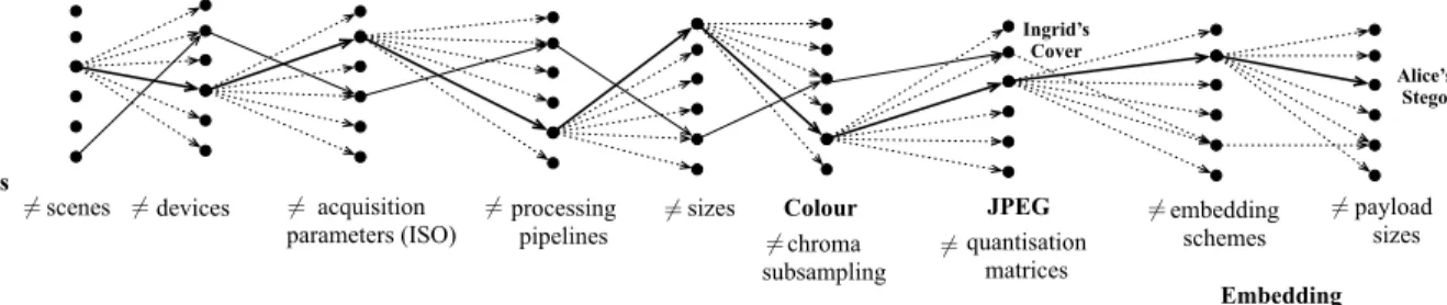
Figure 1: The prisoner’s problem as seen in the ALASKA contest: Eve, the forensics expert, has to face an exponential diversity since each selected parameter is prone to change the distribution of the cover or stego signal. One possible path is associated to one cover or stego image and Eve has to detect Alice’s images from images generated from an Innocent user (Ingrid). training and testing phases, with different devices for each set. In
this competition, the diversity was promoted by using 2 different JPEG Quality Factors (QF), different rescaling ratios, and 2 possible Gamma correction factors. The score used to rank participants was the accuracy (# of correct camera models identification / # of total images). If the outputs of this contest are at the current time still not all published, this contest has been the first to witness the use of deep learning techniques in IFS contests [8].
1.2
A new challenge dedicated to practical
steganalysis
The goal of the ALASKA challenge was to stimulate the develop-ment of new hidden data detection methods dedicated to perform practical, “real-life”, steganalysis; i.e. to detect stego contents in environments which are closer to an operational forensic analyst context.
ALASKA was built from the observation that the vast of majority publications on steganalysis are not based on realistic assumptions, i.e. cannot be used directly by a forensics expert. To support this statement, we analyzed 33 publications on image steganography or steganalysis published in the last 3 editions of IH-MMSec, and from 2016 to 2019 in IEEE-TIFS and IEEE-SPL. From this set we can derive the following statistics:
• 33% of the papers deal with JPEG steganography/steganalysis, other papers focus on sole case of uncompressed images in spatial domain),
• 84% deal with grey-level images (steganalysis in color images was studied, using recent machine-learning-based methods, for the first time in 2014 [16, 26]),
• 70% use only BOSSBase with default development settings as the reference base (CNN-based steganalysis schemes usually perform data-augmentation and tend to use other databases) while it has been recently shown [3, 13] how different pro-cessing tools may change fundamentally the results, • 79% choose onlyPE (the minimum average between false
positive and false negative, assuming number of cover and stego images is the same) as the metric to compute the clas-sification performance,
• 94% perform steganalysis on stego images generated using a fixed embedding rate,
• among the algorithms dedicated to JPEG images, 90% use a constant JPEG quality factor.
These figures show that the typical academic scenario of steganal-ysis is very far from realistic setups. This is due to the fact that the academic world considers steganalysis as a tool to benchmark a steganographic scheme but not as a tool to detect stego images in a realistic environment. This observation is not new: the white paper [23] already mentioned in 2013 the weaknesses of the cur-rent steganalysis schemes and their lack of generalization to more practical configurations, and reference [33] also highlights how the popularity of the BOSSBase database tends to bias the conception of steganographic or steganalysis methods by selecting parameters optimized with respect to this particular database.
We now try to list more practical requirements which stem from more realistic assumptions on the Prisoner’s problem described by Simmons in 1983 [34].
Because Alice’s main goal is to communicate sensitive informa-tion in a stealthy fashion, she needs to act casually and consequently she has to use any random image or set of images, processed using a random pipeline. Alice’s cover images consequently have high prob-abilities to be in color, in JPEG format, to come from an arbitrary device and to be subject to an arbitrary development pipeline.
On the other side, Eve observes transmissions or stored data and potentially has to face a great diversity among images. She has to analyze images coming from different devices, therefore subjected to different acquisition, development and processing pipelines, with different sizes and compressed using different JPEG quantization tables. On top of this, Eve also has to face a wide diversity regarding the steganography, not being aware of the potential embedding scheme, the possible payload and with largely unbalanced testing sets with more cover contents than stego (note that training sets may be balanced easily since Eve can generate stego images).
Additionally, in a vast majority of operational situations, Eve’s detector needs to generate low false positive rates since false posi-tives trigger unnecessary investigations which are time and cost consuming hence undermining the whole detection system. In most cases it is better for Eve not to detect Alice’s communication than to have suspicions about a large number of innocent actors. The prescribed false positive rate one wish to achieve may, in an opera-tional context, depends on the number of scrutinized images and on the consequences of making wrong accusations. One can easily see the terrible impact of having a false positive rate as low as 1% if thousands of images are inspected, generating consequently dozens of false alarms.
This scenario, similar to looking for a needle in a haystack from the Eve’s perspective, is illustrated in Figure 1. Note that this ex-treme diversity is more important than for content based retrieval tasks since the diversity in steganalysis does not come only from the semantic of the image, but also from the invisible components which play an important role in steganalysis. This extreme diversity has been the main motivation behind the ALASKA contest that meant to bring the participant “into the wild”, as for the forensic expert2.
1.3
Main features of the ALASKA contest
Based on the observations presented in the previous section, the main motivation of the ALASKA contest is to propose an “anti-BOSS” contest, which means that this contest must be built to help the forensic steganalyst to detect stego images and not to benchmark the embedding scheme of the steganographer w.r.t. a worst case scenario as it was meant for BOSS. We also wanted to include more realistic uses of steganography and consequently we decided about the following setup3, detailed in the Section 2.
Prescribed false positive rates: Contrary to the BOSS contest which used the average of false alarm and miss detection rates as a ranking metric, we used the miss detection rate for a false positive rate of 5% here (abbreviatedMD5for Miss Detection at 5% false
alarm rate). We think that this metric, which prescribes a given false positive rate and rank steganalysis scheme according to the miss detection rate is more interesting for the forensics expert. This metric was inspired by other metrics:
• FP50 (False positive rate for a miss detection of 50%) which offers interesting statistical properties for centered and sym-metric distributions of cover scores [29].
• “Accuracy at the Top” [24] which gives the accuracy detect-ing one stego content (or actor) among for example the 1% most suspicious contents/actors. This score used to bench-mark search engines is interesting, especially when stego contents are always present in the set of contents under investigation.
In order to be able to compute theMD5, we asked the
partici-pants to rank their images starting with the most suspicious ones. The server computes a threshold allowing 5% of false positives and returned the miss detection rate. During the contest each submis-sion is evaluated over a randomly selected subset of 80% of the testing set. The final results are adjusted with evaluation over the whole testing set.
Diverse color JPEGs: Because the vast majority of images are color JPEGs, we decided to generate cover and stego in the same format, we also consider embedding specific to the JPEG color domain. In order to ease implementation we used only the 4:4:4 chroma-subsamppling format (no subsampling of chrominance). The JPEG are compressed using different standard quality factors. Diverse development pipelines: In order to reflect the great diversity of the processing pipelines we used different development
2The name of the competition comes from the movie “Into the Wild” that takes place in Alaska, USA.
3Note that as explained in the section 4, we noticed that our choices were not all appropriate.
pipelines using RAW images as inputs. Images also are of different sizes.
Different steganographic schemes: We used a set of different embedding schemes which are associated with different payload sizes depending of the image processing pipeline.
2
CHALLENGE SETUP
As emphasized in the introduction, the ALASKA competition was designed to bring steganography and steganalysis practices closer to real-world situations. Such a goal should be enabled with a careful design of the material provided to the competitors and, by extension, to the community. In particular, the pitfalls of the BOSSbase, with its lack of diversity on several fronts, were dully taken into account. Therefore, to motivate the community, beyond the sole ALASKA competition, and to study steganalysis “into the wild” we have designed all competition material following three fundamental pillars:
Diversity: In steganography and steganalysis, diversity of an image base is twofold. First of all, it comes from the diversity of sources of each image. A source, as defined in [14], is identified as a device and a set of algorithms that generates cover content [3, 13]. Consequently, the material must take into account the high diversity not only from the camera devices but also from the processing pipelines of each image. Secondly, diversity comes from the number of different steganographic methods employed to hide information in each image, as well as their settings, mostly the payload of hidden data.
Tunability: Every parameter of the image base should be easily changeable so the practitioner can study the effect of the variation of each parameter independently (e.g : QF, image size, process-ing algorithms, steganographic schemes, etc. . . ). It should also be straightforward to add new parameters. The possibility to tune each and every parameter easily such that one can create a spe-cific dataset for its study is fundamental for future use but may also prevent the adoption at large scale of a uniform and standard dataset.
Future-proofing: The advent of a new paradigm in steganaly-sis, using neural networks and deep learning for instance, requires an image database which is big enough to enable the training of such detectors. Furthermore, all softwares used to generate the image base should be readily accessible without fees, open-source to prevent sudden obsolescence and substitutable to allow easy replacement in case of better alternatives. We deeply believe that providing a very large dataset as well as tools that one can grasp eas-ily is of crucial importance to leverage their use in future research works.
Those three pillars were implemented in practice by providing three different kinds of material:
(1) On the one hand, a training dataset of (almost) 50 000 RAW images taken with 21 different cameras (see details in Ta-bles 1) was made available one month before the kick-off of the competition
(2) On the other hand, for the competition itself, a testing set of 5000 color JPEG images. Competitors had to rank this set
of images from the most likely stego to the most cover and, based on this testing set, we were able to rank the efficiency of competitors methods.
(3) Two scripts were also provided to allow easy conversion from RAW images to JPEG. Those scripts take care, respectively, of the image processing and of the hidden data embedding of each image in a fully automatic fashion. We would like to emphasize that those scripts were made as modular and as tunable as possible. Though the exact processing and embedding process of individual images were unknown to the competitor, the parameters used for the generation of the testing set were also provided allowing the competitor to generate a training set coming from the same sources as the testing set.
The rest of this section motivates and describes precisely each part of the material, namely the RAW image dataset, the processing pipelines of testing set and the steganographic processes that were chosen to generate the testing set.
2.1
The Raw Image Dataset
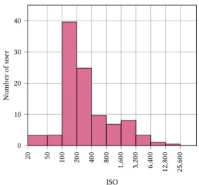
The training set provided on the ALASKA competition webpage was made of 50 000 images in RAW format (several different specific format due to the diversity of cameras). Those images were taken with 21 different cameras as summarized in Table 1. Even though such a number is still far from real word databases, such as FlickR photo-sharing website where hundreds of different cameras can be found, special care was taken to ensure that those cameras spanned every possible sensor size. Thus, images from small, low quality sensors such as the one of an iPad (4.80×3.60 mm) can be found, up to full-frame sensors such as the one found in a Nikon D610 (35.9×24 mm). We also paid attention to include camera models that cover a wide range of technologies through various camera model manufacturers (9 different brands) as well as a large span of production years (from 2003 to 2018). Eventually, we also in-cluded Leica Monochrome as well as full-colour Sigma Foveon X3 sensors. Regarding ISO sensitivity, which as observed in our prior works [13, 14], is the main acquisition parameter that affects ste-ganalysis, we also tried to mimic a realistic dataset with a majority of daily outdoor picture, hence with low ISO; however we have included a non-negligible part of very low ISO, with approx. 6.5% of images with ISO smaller than 100 (that only some camera allows) as well as an important ratio of 13.8% of night or indoor pictures with ISO larger than 1000, see details on the histogram from Fig. 2. Eventually, to include in the RAW image dataset a subset that could mimic the vast diversity one could find in a real practical steganal-ysis setup we have used the photo-sharing website wesaturate4, which allows its users to share photo in various format including raw files and uses a compliant license that allows redistribution. We have downloaded approximately 3 500 images from wesaturate website.
2.2
Image Processing Pipeline
The processing pipeline used in the ALASKA competition was chosen to be as diverse as possible while still producing believable images. To that end, the parameters of each tool in the processing
4see: https://www.wesaturate.com 20 50 100 200 400 800 1 ,600 3,200 6,400 12 ,800 25 ,600 0 10 20 30 40 ISO Numb er of user
Figure 2: Histogram of ISO from raw images.
Camera model #Image year Sensor Size (Mpixels) Canon EOS100D 6979 2013 APS-C (18Mp)
Canon EOS20D 2254 2004 APS-C (8.25Mp) Canon EOS500D 1773 2009 APS-C (15.1Mp) Canon EOS60D 3487 2010 APS-C (18.1Mp) Canon EOS700D 593 2013 APS-C (18Mp)
iPad pro-13” 1899 2015 1/3" (12Mp) Leica M9 1722 2009 FullFrame (18.5Mp) Leica Monochrom 217 2014 FullFrame (18Mp)
Nikon 1-AW 859 2013 1" (14.2Mp) Nikon D5200 4921 2013 APS-C (24.1Mp) Nikon D610 2495 2013 FullFrame (24Mp) Nikon D7100 849 2013 APS-C (24.1Mp) Nikon D90 387 2008 APS-C (12.3Mp) Panasonic DMC-FZ28 1528 2008 1/2.3" (10.1Mp) Panasonic DMC-GM1 2840 2013 4/3" (16Mp) Pentax-K-50 2913 2013 APS-C (16.3Mp) Samsung GalaxyS8 1847 2017 1/2.5" (12Mp) Sigma SD10 2224 2003 Foveon X3 (3x3.5Mp) Sigma SD1Merrill 3320 2011 APS-C, X3 (3x14.8Mp) Sonyα 6000 2667 2014 APS-C (14.3Mp) WorldWideWeb 3525 various various
Total 49299 — —
Table 1: Diversity of Images sources in ALASKA raw images dataset.
pipeline are randomized: the distributions from which they are drawn is fixed and chosen to avoid aberrant looking images while providing extremely diverse image sources.
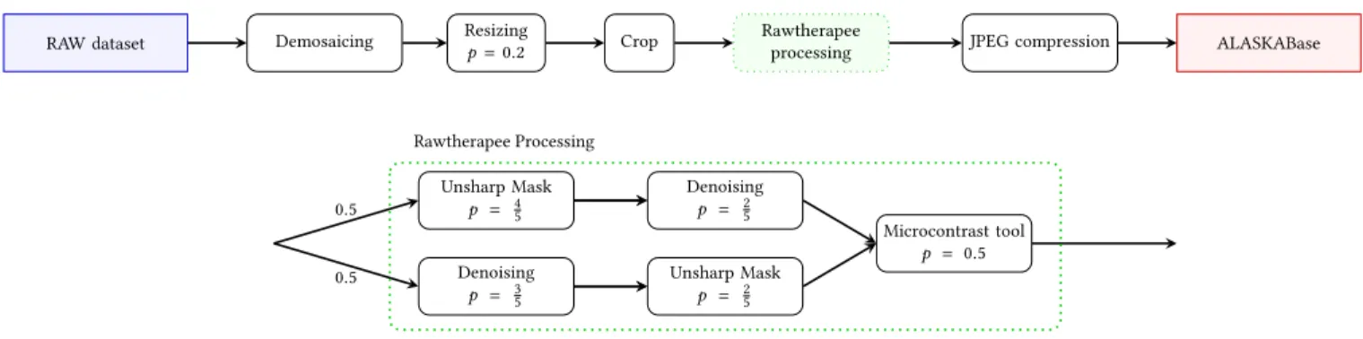
This image development and processing pipeline is depicted in Figure 3 and details in what follows:
Demosaicking: The first step in the processing pipeline is to apply demosaicking on the image. This was done using Rawthera-pee5v5.4 by selecting randomly and for each image individually, one among the four following algorithms (the probability for choos-ing a given algorithm is given between the brackets): AmAZE (40%), DCB (30%), IGV (15%), Nearest-neighbor or Fast interpolation (15%).
RAW dataset Demosaicing Resizingp = 0.2 Crop Rawtherapee
processing JPEG compression ALASKABase
Unsharp Mask p = 4 5 Denoising p = 2 5 Denoising p = 3 5 Unsharp Mask p = 2 5 Microcontrast tool p = 0.5 0.5 0.5 Rawtherapee Processing
Figure 3: Processing pipeline followed for each image from the RAW database up to JPEG compression. The second figure details the different Rawtherapee processes. Thep value gives the probability that a given process is applied, when it is absent, the process is always applied.
AmAZE and DCB were chosen and associated with highest proba-bilities because they are currently the most popular options with Rawtherapee users due to their extremely good results with few artifacts. IGV was the algorithm that, during our benchmarks, con-sistently gave images that were hard to steganalyze and the nearest neighbor interpolation was chosen as a alternative for users aiming at speed up processing time. Images were then saved as 16-bit TIFF using python’s Pillow library6.
Resizing: Following demosaicking, resizing is applied to the image with 20% probability using a 8x8 Lanczos filter. The resize factor is comprised between 60 and 130 and chosen from a gamma distribution with pdfP(x, a = 10) = j100 ·j0.08 ·xa−1Γ(a)exp(−x)k k rectified on [60, 130].
Smart Crop: As a third step, the image is cropped following the so-called “smart crop” process defined in [37]. Let us briefly recall that one of the main issue when cropping randomly an image is to avoid extracting a subpart with dummy content, typically a portion with all pixels overexposed for instance. The idea proposed in [37] is to extract a portion in which residuals has approximately the same distribution as the overall image. For ALASKA challenge, we used this “smart cropping” technique to reduce each dimension, width and height, to a random size, drawn from uniform distribution, among the four following sizes: {512, 640, 720, 1024}.
Denoising, sharpening, micro-contrast: Once cropped, the image is subjected to various images processes using RawTherapee, as summarized in Figure 3: Each image can be sharpened, using the well-known Unsharp Mask (USM) algorithm, and/or denoised, us-ing Pyramid Denoisus-ing based on wavelet decomposition; eventually we may apply a micro-contrast local edge enhancement tool, that prevents introducing halo artifacts often present when using USM. Every step is selected or skipped with a fixed probability indicated in Figure 3 and, if selected, the specific parameters of each tool are drawn randomly from distributions which were chosen empirically
6available at: https://pillow.readthedocs.io/en/5.1.x/
to get a good balance between image difficulty, diversity and be-lievability. Those specific distributions as well as their parameters are reported in Appendix A.
JPEG compression: Eventually, each image is compressed fol-lowing the JPEG standard using the Pillow library. To set the pa-rameters of the JPEG compression we used a dataset of 2 691 980 JPEG images downloaded from FlickR [40] that were compressed using one of the standard quantization tables. We noted that those images were, in more than 85% of cases, not subject to Chroma subsampling. Therefore, we have chosen not to use Chroma sub-sampling. However the JPEG quality factor was drawn in such a way as to match closely the empirical distribution of QF observed on the dataset downloaded from FlickR. The probabilities of using each and every JPEG QF are presented in Appendix A.
2.3
Steganographic Embeddings
We detail now the different components related to the stegano-graphic part: selection of the embedding methods, the choice of the payload size w.r.t. the image size, the allocation of the payload between the different color channels and the benchmark used to tune the different parameters.
Stego schemes: Bringing steganalysis closer to operational con-text means that the embedding methods must be very diverse, draw-ing as much from state-of-the-art adaptive embedddraw-ing schemes as from older, weaker schemes such as naive LSB replacement. Con-sequently we selected four embedding schemes from the old non-adaptive nsF5 [11] to recent non-adaptive schemes such as UED [18] and EBS [39] including the current state-of-the-art J-UNIWARD [20].
Payload size w.r.t. image processing pipeline: In a realistic operational context, Alice and Bob want to share a given size of data; this could be transformed for the ALASKA competition to a fixed embedded size. However, this may lead to a situation in which a non-negligible fraction of the steganographic contents will be hardly detectable (for instance, strongly sharpened images using state-of-the-art embedding schemes) while, on the opposite, for other images the detection will turn out to be obvious (e.g. denoised images with non-adaptive scheme).
or less the same difficulty when it comes to detecting their stego content. While the principle is quite simple, this turns out to be very difficult in practice since it requires finding for each image source a relevant payload to achieve the targeted “steganalysis difficulty”. While models may allow to do so for spatial domain [32, 38], prior works in JPEG domain are far less developed.
To determine such a payload for all possible image sources we adopted the following methodology:
• First of all, from a subset of 10, 000 images, including the raw images from testing set, we generated several variations of the same dataset, each developed in a different fashion. More specifically, we have generated all sets of different sources using a specific developpement pipeline combining: (i) 4 demosaicking algorithms (ii) 3 possible resizing factors (iii) 3 edge enhancement strengths (iv) 3 image denoising strengths and (v) 4 different JPEG quality factors, those were 100, 97, 90 and 80. See also the processing pipeline in Figure 3. • Second, we have developed a tool that, using an improved version of secant lines, allows finding for a given set of im-ages from the same source the average payload that achieves the desired difficulty ; this payload that on a given dataset matches with a prescribed steganalysis error rate is refered to as the “secure payload” in [32, 38]. Because the ALASKA competition focuses on theMD5criterion of detection
per-formance, we targeted aMD5of 65%.
However the main shortcoming of this methodology is that the combination of all the possible developments leads to a combinato-rial explosion with 4 × 3 × 3 × 3 × 4= 432 different images sources to generate and, with 4 embedding schemes, a total of 1728 payloads to determine. Because such a number is completely out-of-reach, we simplified the estimation by assuming that the demosaicking step has only a negligible influence. Consequently it was not considered. For further simplification we computed the payload only for a few of those cases and made a linear regression for each parameter individually.
However, because even without taking into account the demo-saicing, considering all possible combinaisons of processings lead to 432 sources. We have not been able to determine numerically all possible payload, that matches the requiredMD5of 65%, and
there-fore used the available results through a simple linear regression (for each parameter individually, regardless the other parameters). Only for the JPEG quality factor we have noted that this parameter seems to be hardly modelled using a linear model and, hence, shift to a model in which this parameters has an exponential impact on the “secure payload”.
Payload size w.r.t. image size: Eventually, regarding image sizes, we have deliberately chosen to adopt a simple square root law (SRL [9, 21, 25]) which, accounts neither for the coding strategy nor for the cost associated with each pixel. Indeed, a more accurate (not-so-square-root) law, that adapts the payload as a function of images size, for adaptive embedding schemes and using advanced coding scheme [22] does seem hardly applicable in practice [15]. Obviously, see section 3.2 and more precisely Figure 11, a “naively” use of the Square Root Law leads to the result that one may expect:
the payload is underscaled for larger image sizes.
Payload repartition among color channels: Although the vast majority of digital images are color images compressed in JPEG, using three channels (Y , CbandCr), recent works in steganalysis focus almost exclusively on grayscale and uncompressed images (see Section 1.2). It was therefore fundamental for us to find a trade-off between moving towards a practical scenario and running a competition in line with recent developments in steganalysis.
We consequently decided to modify the classical embedding scheme by spreading the payload size between the different com-ponents. The question related to the best way to spread a payload ofP bits among the channels Y , CbandCr for 4:4:4 sampling ra-tios is investigated in [36] from a practical perspective. The au-thors propose to tune a parameterβ ∈ [0; 1] that balances the payload allocated to the luminance and chrominance channels w.r.t. the practical security. For example,β = 1 implies that all the payload is conveyed by the two chrominance components and β = 0 implies that the payload is embedded in the luminance component only. More specifically, givenPY,PCb andPCr the
pay-load sizes for each channel, the authors of [36] propose to use the following relations:PY = γ (1 − β)NY,PCb = γ βNCb/2 and
PCr = γ βNCr/2, whereNY,NCb andNCr are respectively the
number of non-zero AC coefficients for theY , CbandCr channels andγ is a proportionality factor to ensure that PY + PCb+ PCr
equals the desired overall payload. However, we made an implemen-tation mistake (as it has been confirmed by independent works from participants [43]) by computingPY = γ (1 − β)(NY + NCb+ NCr) andPCb = PCr = γ β(NY + NCb+ NCr)/2.
Note that this change tends to allocate a larger payload into chrominance channels and consequently decreases the practical security. For example, for a typical image at QF75 whereNY =
10000,NCb = 1000, NCr = 1000, if we set P = 1000 bits, β = 0.4
we obtainPY = 882 bits and PCb = PCr = 59 bits using spreading
presented in [36] vsPY = 600 bits and PCb = PCr = 200 bits for
our implementation.
Practical security assessment: The payload size was evalu-ated empirically based on basic and fast steganalytic tests. The experiments were conducted using the DCTR (Discrete Cosine Transform Residual) [19] features set concatenated from each color channels [36] together with the low-complexity linear classifier from [4] (LCLC). This choice was based on the need to get as many payload evaluation as possible in the least amount of time.
With this approach, we were able to provide a “lower” and “up-per” bounds on the detection accuracy one may get under our experimental framework. The “lower bound” corresponds to the performance one gets when naively training and testing DCTR and the LCLC directly on the material provided for the competition. We get a results ofMD5≈ 0.795, that is, approximately 80% of missed
detection for a false alarm rate of 5%.
The “upper bound”, on the other hand, corresponds to the best achievable results when using DCTR and the LCLC. Our hypothesis was that the best achievable results would be those obtained in the absence of any cover-source mismatch. This would amount to train one detector per source in the testing set which would have been impossible to do in the time frame leading to the competition. We
Date Aug. Sept. Oct. Nov. Dec. Jan. Feb. Mar. Total Visits 688 4046 4205 4650 5452 4533 4115 2379 30068 TX (TB) 69 60 18 22 13 6 19 1 208
Table 2: Usage of the website of alaska.utt.fr per month, in terms of the number of unique daily visits and transmitted data volume (TX). Aug. Sep . Oct. No v. De c. Jan. Feb . Mar . 0 100 200 300 400 date (day) Numb er of users and submissions Users Submissions
Figure 4: Evolution of the number of registered users (blue) and number of submissions (green).
thus went under the assumption that our regression and evaluation method has a reasonable accuracy meaning that the best achievable MD5should be close to the targeted one set to 0.65.
3
CHALLENGE RESULTS AND ANALYSIS
After having described in details the goals, the setup and the orga-nization of the ALASKA challenge, we present in this section what happened during the contest and how the competitors performed.
3.1
Timeline and website usage
First of all, we would like to present the usage of the website alaska.utt.fr.
Table 2 presents the volume of data sent by the server (TX, in Tera Bytes) as well as the number of unique daily connections that have been recorded on the website server. Note that, for this counter, we do not only count the individuals that visits the website, but instead each and every connection to the website server. While the former case includes only visits through a website, the latter case accounts for downloads of image datasets, and also for attackers who attempt to grant access to the server (usually from a few attacks up to a few dozens a day).
Similarly, Figure 4 presents the number of registered users (in blue) as well as the number of submissions (in green). Quite unsur-prisingly, this figure shows different trends between the number of users and number of submissions that perfectly matches with the observations from Table 2.
Though the final number of submissions, over 400, is quite impor-tant, we wanted to look at the number of submissions per individual. The histogram of the number of submissions per individual users is presented in Table 3. First of all, the main conclusion one may draw out of this table is that a vast majority of users (242 out of 285) did not make submission. Note that we only count here the “active”
Nb of Submissions Nb of Users 0 244 1–5 25 6–10 6 11–15 4 16–20 2 21–25 0 26–30 3 31–35 2 36–40 0 41–45 0 46–50 2 Total 285
Table 3: Number of number submission per users.
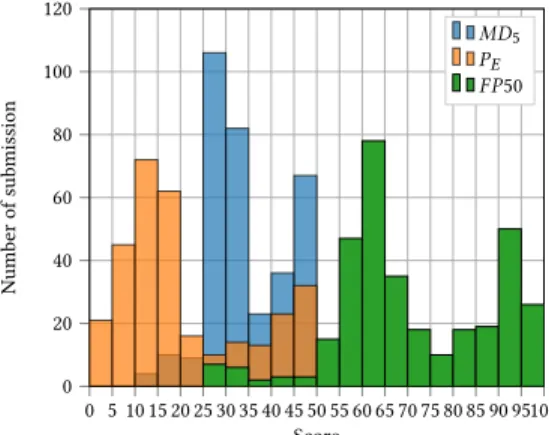
0 5 10 15 20 25 30 35 40 45 50 55 60 65 70 75 80 85 90 95100 0 20 40 60 80 100 120 Score Numb er of submission MD5 PE FP50
Figure 5: Number submissions as a function of performance w.r.t the three criteria used (MD5,PE and FP50).
users whose account was validated using an email confirmation system. Two explanations may be found for this very high number of non-participating users. First of all, it is likely that many users registered only to get access to the material provided (the image datasets as well as the development scripts provided, see Section 2 for details). Another possible explanation that may be found is that some users downloaded the dataset, quickly tried to evaluate offline the performance of their detection system and, not being able to compete with the top competitors, gave up without submission any answers.
3.2
Comparison between competitors
Let us now present describe how the competitors performed. Fig-ure 5 provides a general overview of the distribution of perfor-mances over all the submissions. Here, as reported during the com-petition on the website, we report the results using three distinct criteria, the usualPEas well as theFP50 and the MD5, both
pre-sented in Section 2, the letter being the only one used to rank competitors.
The first comment one may have when observing the Figure 5 is thatPE as well asPF 50 are not very discriminative. This can be explained, in part, because such performance metric lie in the range (0, 0.5); on the opposite theMD5lies in the range (0, 0.95). Note also
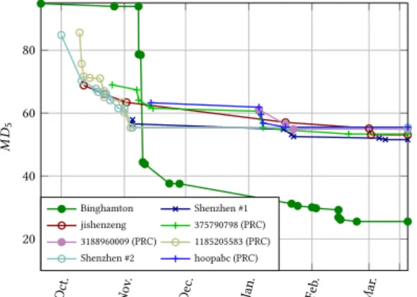
Competitor MD5 PE FP50 yyousfi / Binghamton Univ. 25.2% (24.37%) 14.49% 0.71% 2016130231 / Shenzhen Univ. 51.6% (50.00%) 25.50% 5.67% 3188960009 / PRC 53.8% (54.93%) 26.33% 7.66% 375790798 / PRC 54.2% (53.35%) 25.78% 7.56% Table 4: The Hall of Fame (as of March 14th): top 5 com-petitors by the end of ALASKA competition. Note that those scores correspond to the best results for each criterion indi-vidually and were computed over all images while, on the opposite, the results published online through alaska.utt.fr were computed on a random subset and are reported in brackets forMD5. Oct. No v. De c. Jan. Feb . Mar . 20 40 60 80 M D5 Binghamton Shenzhen #1 jishenzeng 375790798 (PRC) 3188960009 (PRC) 1185205583 (PRC) Shenzhen #2 hoopabc (PRC)
Figure 6: Evolution of the scores of the eight best competi-tors.
that theFP50 has been designed for “very reliable” detection with extremely low false alarm rate; such a criterion is therefore more relevant to distinguish detectors with false alarm rate of 10−6and 10−4, which does not fit quite well with the context of a competition such as ALASKA where it would require to train and test on dozens of millions of images.
Figure 5 also emphasizes the challenging aspect of moving ste-ganalysis “into the wild” with an important fraction of detection results below the “upper” bound of 65% when using off the shelf fast features-based machine learning tools. Eventually, one can observe clearly a group of submission substantially ahead, they all come from the winning team from Binghamton University. All other competitors that went seriously into the competition has seen their performance, in terms ofMD5plateauing between 52% and
58%. This can actually be observed for any of the three performance criteria.
We also wanted to present the evolution of the score for the top competitors in Figure 6. We picked the eight top scorers because we observed that including more users would not bring any more information while bringing more confusion by putting too many values into same graphs. From this figure, the first thing we can note is the strategy of the team from Binghamton University that starts entering the competition “seriously” once they have detec-tion methods that largely outperform the other competitors by a margin of 15%. We can also observe a group of three competitors (from which two at least are from ShenZhen University) who were
quickly able to reach approx. aMD5of 55% while hardly being
able to improve this score over the four remaining month of the competition. A notable exception is ShenZhen team #1, who un-der username “2016130231”, managed to improve its performance slowly to eventually end up at the second place. Eventually, we can also note a third group of users who started to reach the “lower” bound of 65% by November but constantly managed to improve the performance to end up with the same results as the second group of users.
3.3
Results analysis
As introduced in the previous section, it is interesting to look at the results obtained by the best competitors for different types of images. In particular, we want to uncover if some users specifically target a specific kind of covers. To this end we propose to show the results obtained by the competitors with respect to six individ-ual features; those are (ordered as in the processing pipeline, see Figure 3), the demosaicking algorithm, the resizing factor (if used), the image processing tools (denoising and edge enhancement), the image size and the JPEG quality factor.
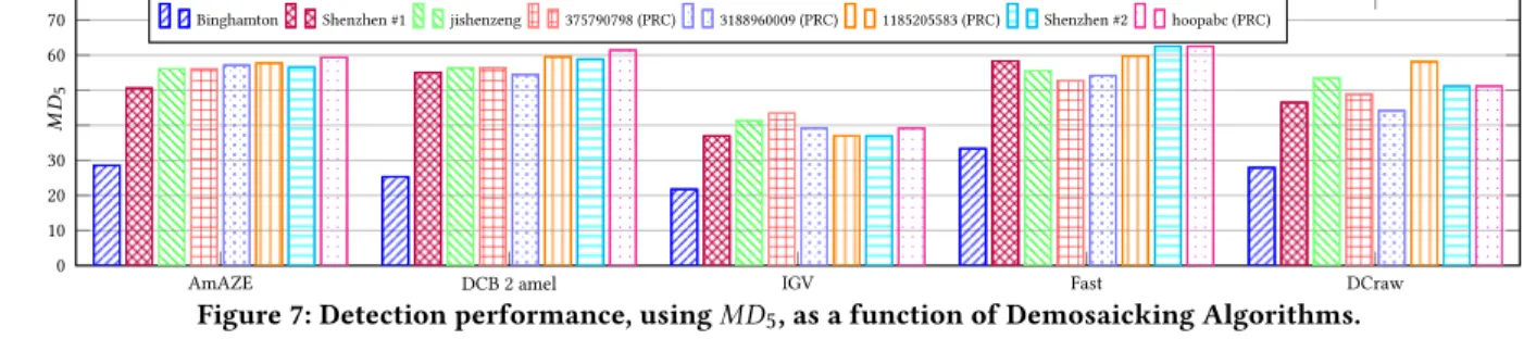
Impact of demosaicking: The results from the competitors for various demosaicking algorithms are reported in Fig 7 which, as the next figures 7–13, put together the results obtained by different users for the same subset of images. In Figure 7 the five set of results gathered are for each and every demosaicking algorithm. We observe that the accuracy of the detection loosely depends on the demosaicking. A notable exception to this is the IGV algorithm for which theMD5drops by a factor of approximately a third for all
users. We also note that the “DCraw” demosaicking had been added due the presence of images shot with a Sigma full-color Feveon X3 sensor which is not supported by rawTherapee. Interestingly, the results of the competitors in this dataset are more heterogeneous, possibly because the image processed using DCraw represents a rather small fraction of the training and testing sets.
Impact of resampling: Figure 8 show the results obtained by the competitors depending on the presence or absence of resam-pling. For a vast majority of the competitors, one can observe that resizing has almost no impact on steganalysis performance. A no-table exception, however, can be observed from the leading team whoseMD5increases by more than 25% on resampled images.
It is worth noting that resizing has been used for only one fifth of the image, see Figure 3, therefore, it is likely that the learning methods focus somehow on the vast majority of non-resampled images.
Impact of filtering: The next step of the raw file development pipeline is the image processing, namely denoising and edge en-hancement, or sharpening; the results of steganalysis performance from top submissions, as a function of the “strength” of those pro-cessing tools, are given in the Figures 9 and 10.
Regarding the impact of edge enhancement, one can observe that the inserted payload is slightly too small when this processing is not used hence the higherMD5for all competitors. However
it is striking that all competitors have performance that loosely depends on the strength of edge enhancement. A notable exception
AmAZE DCB 2 amel IGV Fast DCraw 0 10 20 30 M D5 60
70 Binghamton Shenzhen #1 jishenzeng 375790798 (PRC) 3188960009 (PRC) 1185205583 (PRC) Shenzhen #2 hoopabc (PRC)
Figure 7: Detection performance, usingMD5, as a function of Demosaicking Algorithms.
No Resizing Image resizing (resampling) 0 10 20 30 M D5 60 70
80 Binghamton Shenzhen #1 jishenzeng 375790798 (PRC)
3188960009 (PRC) 1185205583 (PRC) Shenzhen #2 hoopabc (PRC)
Figure 8: Users detection accuracy as a function of resizing. to this behavior comes, once again, from the leading team from Binghamton University. Indeed theirMD5is doubled when shifting
from light to strong edge enhancement, while, on the opposite, it remains almost constant for all other competitors.
Impact of the image size: The ultimate step of the develop-ment pipeline is the choice of image size. As explained in the Sec-tion 2.3, we adopt a simple SRL (Square Root Law) under which the square root of the message length is set proportional to the number of DCT coefficients. The results presented in Figure 11 go exactly along the same direction as the previous analysis: all users achieved significantly higher missed detection ratesMD5, for larger image
sizes.
Impact of JPEG QF:. Eventually, the very last step of all pro-cessing pipelines is the compression. Figure 12 show the results obtained by the competitors as a function of the JPEG Quality Factor (QF). Our evaluation of the relevant payload to ensure a constant difficulty for steganalysis did not work really well for this parame-ter. This is probably due to the fact that, as opposed to the other parameters of the processing pipeline, it seemed hardly possible to map the QF to the “secure” payload [32] using a linear relation, given the few results we had for this evaluation. Therefore we have picked an exponential relation from the QF to the secure payload which appears, retrospectively, rather inaccurate.
Beside the fact that the difficulty of steganalysis greatly increases with the QF, another very interesting phenomenon one can observe from Figure 12 is the notable exception to this rule from Binghamton Team. Indeed while difficulty for all user is maximal for images with the highest QF, for those images the team from Binghamton have achieved almost perfect detection, highlighted on this figure with a very lowMD5, that is a missed detection rate of about 3% for 5%
of false-alarm. In fact, over the 782 images with QF 100, this team made only 2 errors. Obviously, a novel attack has been discovered, see more detail in their paper [43].
Impact of the embedding scheme: As explained in Section 2.3, the embedding was designed to make each scheme equally
difficult. This is reflected in Figure 14 where the performance of the competitors is stable across all steganographic schemes with the notable exception of nsF5. Indeed every competitors performs the worst on nsF5 which is actually the weakest scheme used in ALASKA. While the exact reasons of this phenomenon still elude the authors, several facts about the way nsF5 was used during the competition might explain it. First of all, nsF5 embeds only in non-zero AC coefficients (nzAC). If every image of the ALASKA test set (5000 images) was embedded with nsF5, approximately 150 would not have enough nzAC for embedding with approximately 30 of them resulting in no changes in at least one the three color channels. Since the test only contained 500 stego images with only 15% of them being nsF5, such an event is still quite rare and cannot explain the huge loss inMD5for all competitors. More interesting, however,
is the fact that nsF5 simulates embedding with optimal coding. Given that the base payload of nsf5 for the competition is already quite low at 0.04 bpp, the embedding efficiency is excellent (8.5 on average) meaning that the number of changes in the chrominance channels will always be small (in the order of hundreds). While this might not have been a problem for the rich models used for benchmarking the competition, the neural networks used by the competitors all needed curriculum training to account for small payloads. Since the payload of nsF5 was far smaller than the other schemes, its is possible that it was not taken into account as well as the others schemes during the training phase by the networks.
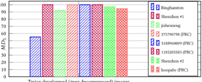
The return of the Cover-Source Mismatch: Apart from the processing pipeline itself, two interesting splits of competitor results according to image sources can be presented. Indeed, we included a small subset of 400 images that were directs output by cameras as JPEG images. The goal of this subset of images, which were absent from the training set, was to be able for us to measure easily how much each competitor methodology has the ability to be general-ized to images coming from slightly different sources. However to avoid putting images that come from sources that largely differs from the ALASKA training set, those 400 images were jpeg decom-pressed and subject to same pipeline, depicted in Figure 3, with the exception of the demosaicking.
The results presented in Figure 13 show that a vast majority of competitors can hardly adapt to this CSM, with missed detection MD5of over 90%, and even reaching 100% for half of the
competi-tors.Binghamton’s team also suffers from the CSM of this subset of images but to a much lesser extend.
No Edge Sharpening light Edge Sharpening Medium Edge Sharpening strong Edge Sharpening 0 10 20 30 M D5 60 70
Binghamton Shenzhen #1 jishenzeng 375790798 (PRC) 3188960009 (PRC) 1185205583 (PRC) Shenzhen #2 hoopabc (PRC)
Figure 9: Detection performance, usingMD5, as a function of Unsharp mask strength on images.
No Denoising Light Denoising Strong Denoising 0 10 20 30 M D5
60 Binghamton Shenzhen #1 jishenzeng 375790798 (PRC) 3188960009 (PRC) 1185205583 (PRC) Shenzhen #2 hoopabc (PRC)
Figure 10: Detection performance, usingMD5, as a function of images denoising.
Small images (< 400kpix.) Med. size images (400k << 550kpix.) Large images (> 650kpix.) 0 10 20 30 M D5 60 70
Binghamton Shenzhen #1 jishenzeng 375790798 (PRC) 3188960009 (PRC) 1185205583 (PRC) Shenzhen #2 hoopabc (PRC)
Figure 11: Detection performance, usingMD5, as a function of images size.
60≤QF≤80 80 < QF≤ 90 90 < QF≤ 98 98 < QF≤ 100 0 10 20 30 M D5 60 70
80 Binghamton Shenzhen #1 jishenzeng 375790798 (PRC)
3188960009 (PRC) 1185205583 (PRC) Shenzhen #2 hoopabc (PRC)
Figure 12: Detection performance, usingMD5, as a function of jpeg QF .
4
MAIN LESSONS AND CONCLUSIONS
During this whole adventure, we had the satisfaction to notice that there were no major problems with the design of the contest, that it was neither too difficult, nor too easy. Still if we could use a time-machine, we would change at least two things:
(1) We would fix the error we made on payload allocation in the Chroma channels (see section 2.3) in order to reduce the detectability of the whole system. The positive outcome of this mistake is to show how carefully the embedding must to be done on color images.
(2) We would also generate cover and stego images that are more realistic. As it is illustrated on Figure 15, since we cropped images, potentially exotic developments, and because our
“smart-crop” scheme was not efficient enough, a large pro-portion of our dataset was not representative of a typical set of images found on a social network or on a hard-drive. We could fix this problem by using important downscaling operations and minor cropping instead.
Organizing the ALASKA has been also very time consuming and put a lot of stress upon all our shoulders7. For instance when we realized on August 29th at 1:30 am that one of the image processes was skipped (merely because some silly guy, the second author, commented it in the script) or when after having strive to get all the materials ready for September 1st, Andreas Westfeld burnt
Twice developped (jpeg decompressed) images 0 10 20 30 M D5 60 70 80 90 100 Binghamton Shenzhen #1 jishenzeng 375790798 (PRC) 3188960009 (PRC) 1185205583 (PRC) Shenzhen #2 hoopabc (PRC)
Figure 13: Detection performance, usingMD5, for jpeg
de-compressed images ; note that those images have been sub-jected to same image processing pipeline, see Figure 3, ex-cept for the demosaicking.
instantly all our efforts to the ground by finding that stego and cover images had different timestamps8. . .
However, organizing ALASKA was also a lot of fun during which we have many times ask ourselves many open questions. While some very interesting research outcomes have already pop up from ALASKA competition, we are deeply convinced that the contest brought the focus on many open questions and may pave the way to even more interesting research works.
It is hard to stop such an exciting adventure, therefore we will propose soon a follow-up competition with the same idea of bring-ing steganalysis closer to the “real life” operational context. This follow-up competition will certainly be hosted on Kaggle in order to allow as many user as possible from different fields, with hope-fully a decent cash price as well as a larger dataset of more than 75.000 raw images from more than 30 camera models that should be available for ACM IH&MMSec’19 conference. This follow-up competition should also go wild in the sense that we will try to design a more realistic yet more diverse image processing pipelines to provide the community with datasets that resemble those one can find on the Internet.
ACKNOWLEDGMENTS
All the source codes and images datasets used to obtained the results presented will be made available on the Internet upon acceptance of the paper. The (raw) images dataset as well as the codes used for conversion to JPEG and application of several processing pipeline are already available at: https://alaska.utt.fr. This work has been funded in part by the French National Research Agency (ANR-18-ASTR-0009), ALASKA project: https://alaska.utt.fr, and by the French ANR DEFALS program (ANR-16-DEFA-0003).
We would like to thank all the individuals that help us organizing this contest. Those are mainly (but not exclusively):
• Antoine Prudhomme, for creating the website https://alaska. utt.fr ;
• Julien Flamant, Jean-Baptiste Gobin, Florent Pergoud, Luc Rodrigues and Emile Touron for kindly providing some of their raw images that we redistributed (with their agreement) during this challenge.
8Andreas Westfeld also find another attack on the submission system which originally accepted non-integer image indices
• Andreas Westfeld for striving hard to burn our effort to the ground and helping us this way to improve the “security” of the competition website.
• The computer resources department of Troyes University of Technology who helped us with all their advices and suggestions.
A
RAWTHERAPEE PROCESSING DETAILS
In this appendix we detail the different processes used in the sharp-ening and denoising set as described in Section 2.2. In particular we explain how the parameters of each tool was chosen randomly by sampling from some fixed distribution as well as the rationale behind our choices. More information about each tool can be found in the Rawtherapee document at http://rawpedia.rawtherapee.com. Three tools from Rawtherapee v5.4 were chosen as processing that tended to introduce cover-source mismatch when not taken into account :
Unsharp Mask: A well-known sharpening tool used to increase the edge contrast in images. It informally works by substracting a blurred version of the original image from the original image.
Directionnal Pyramid Denoising: A denoising tool which uses a multi-resolution representation of the image.
Microcontrast tool: An ad-hoc algorithm in the Rawtherapee sharpening suite used to sharpen edges while not introducing any halo artifact.
Each tool is controlled by a set of parameters. During the dataset generation and for each image processed, we sample the values of each one of those parameters from distributions designed to give a good trade-off between diversity and believability of the resulting image. This means that distributions were chosen such as the extreme values of the parameters are usually avoided (but possible) while still keeping the variance of those parameters as high as possible.
A.1
Unsharp Mask
The Unsharp Mask tool (USM) is controlled by three parameters : Radius: The Radius determines the size of the details being amplified and consequently, relates to the width of the sharpening halo. It is the radius of the Gaussian blur. The radius follows a normal distribution N (1.5, 1) rectified on [0.3, 3]
Amount: The Amount (percentage) parameter controls the strength of the sharpening. It follows a normal distribution ⌊N (500, 200)⌋ rectified on [0, ∞[
Threshold: The Threshold values are left at default (20, 80, 2000, 1200), threshold is a parameter to confine the sharpening to a desired space (the stronger edges), in RawTherapee, the threshold is a function of luminance, the default values specify little sharpening in the black-est tones, high sharpening at lighter tones and then less sharpening at the lightest tones.
A.2
Directionnal Pyramid Denoising
The denoising tool is controlled by two parameters (chroma denois-ing is set as automatic) :
Luminance: Luminance follows a gamma distributionP(x, a = 4)= 100 · 0.1 ·xa−1Γ(a)exp(−x)rectified on [0, 100] and controls the strength of the noise reduction
J-UNIWARD EBS UED nsF5 0 10 20 30 M D5 60 70
Binghamton Shenzhen #1 jishenzeng 375790798 (PRC) 3188960009 (PRC) 1185205583 (PRC) Shenzhen #2 hoopabc (PRC)
Figure 14: Detection performance, usingMD5, as a function of the embedding scheme.
Figure 15: Montage of 50 images having very poor semantic contents picked from the first thousands images (5%).
Figure 16: Repartition of the images w.r.t. JPEG QF on the FlickR website [40] and for the Alaska testing base. Detail: Detail follows a uniform distribution U({0..60}) and
controls the restoration of the textures in the image due to excessive denoising.
A.3
Microcontrast tool
The microcontrast is controlled by two parameters :
Strenght: Strength follows a gamma distributionP(x, a = 1) = j
100 · 0.5 ·xa−1Γ(a)exp(−x)k rectified on [0, 100], it tunes strength of the sharpness applied (how many adjacent pixels will be searched for an edge)
Uniformity: Uniformity follows ⌊N (30, 5)⌋ rectified on [0, ∞[, it tunes the level of the microcontrast enhancement.
A.4
JPEG QF
As described in Section 2, we have drawn the JPEG QF from a distribution that mimics the one observed empirically on the large FlickR [40] dataset as it should reveal what one shall find in a practical operational context.
We report in Table 16 the number of images downloaded that match each and every standard QF from 50 to 100. For comparison we present the probability we have used for all QF from 60 which, for simplification purpose, has been rounded to 0 whenever it was smaller than 0.1%.
Note that we only report the numbers for downloaded images that match the JPEG standard quantization tables, which represents approximately 2.7 million images but only less than 15% of total number of downloaded images.
REFERENCES
[1] P. Bas, T. Filler, and T. Pevný. 2011. Break Our Steganographic System — the ins and outs of organizing BOSS. In Information Hiding, 13th International Workshop (Lecture Notes in Computer Science). LNCS vol.6958, Springer-Verlag, New York, Prague, Czech Republic, 59–70.
[2] P. Bas and A. Westfeld. 2009. Two key estimation techniques for the Broken Arrows watermarking scheme. In MM&Sec ’09: Proceedings of the 11th ACM workshop on Multimedia and security. ACM, New York, NY, USA, 1–8. [3] D. Borghys, P. Bas, and H. Bruyninckx. 2018. Facing the Cover-Source Mismatch
on JPHide Using Training-Set Design. In Proceedings of the 6th ACM Workshop on Information Hiding and Multimedia Security (IH&MMSec ’18). ACM, New York, NY, USA, 17–22.
[4] R. Cogranne, V. Sedighi, J. Fridrich, and T. Pevný. 2015. Is Ensemble Classifier Needed for Steganalysis in High-Dimensional Feature Spaces?. In Information Forensics and Security (WIFS), IEEE 7th International Workshop on. 1–6. [5] P. Comesaña, L. Pérez Freire, and F. Pérez-González. 2006. Blind Newton
Sensi-tivity Attack. IEE Proceedings on Information Security 153, 3 (September 2006), 115–125.
[6] D. Cozzolino, D. Gragnaniello, and L. Verdoliva. 2014. Image forgery detec-tion through residual-based local descriptors and block-matching. In 2014 IEEE international conference on image processing (ICIP). IEEE, 5297–5301. [7] D. Cozzolino, D. Gragnaniello, and L. Verdoliva. 2014. Image forgery localization
through the fusion of camera-based, feature-based and pixel-based techniques. In 2014 IEEE International Conference on Image Processing (ICIP). IEEE, 5302–5306. [8] D. Cozzolino and L. Verdoliva. 2018. Noiseprint: a CNN-based camera model
fingerprint. arXiv preprint arXiv:1808.08396 (2018).
[9] T. Filler, A. D. Ker, and J. Fridrich. 2009. The Square Root Law of Steganographic Capacity for Markov Covers. In Media Forensics and Security XI, Proc SPIE 7254 (SPIE). 801–0811.
[10] J. Fridrich and J. Kodovsky. 2012. Rich models for steganalysis of digital images. Information Forensics and Security, IEEE Transactions on 7, 3 (2012), 868–882. [11] J. Fridrich, T. Pevný, and R. Kodovský. 2007. Statistically Undetectable Jpeg
Steganography: Dead Ends Challenges, and Opportunities. In Proceedings of the 9th Workshop on Multimedia & Security (MM&Sec ’07). ACM, New York, NY, USA, 3–14.
[12] T. Furon and P. Bas. 2008. Broken Arrows. EURASIP Journal on Information Security 2008 (Oct. 2008), ID 597040.
[13] Q. Giboulot, R. Cogranne, and P. Bas. 2018. Steganalysis into the Wild: How to Define a Source?. In Media Watermarking, Security, and Forensics (Proc. IS&T). 318–1 – 318–12.
[14] Q. Giboulot, R. Cogranne, D. Borghys, and P. Bas. 2015. Roots and Solutions of Cover-Source Mismatch in Image Steganalysis: a Comprehensive Study. (submit-ted), 1–4.
[15] Quentin Giboulot and Jessica Fridrich. 2019. Payload Scaling for Adaptive Steganography: An Empirical Study. submitted, 1–4.
[16] M. Goljan, R. Cogranne, and J. Fridrich. 2014. Rich Model for Steganalysis of Color Images. In Proc. IEEE WIFS. Atlanta, GA, USA.
[17] G. Gul and F. Kurugollu. 2011. A new methodology in steganalysis: breaking highly undetectable steganograpy (HUGO). In International Workshop on Infor-mation Hiding. Springer, 71–84.
[18] L. Guo, J. Ni, and Y. Q. Shi. 2012. An efficient JPEG steganographic scheme using uniform embedding. In Information Forensics and Security (WIFS), 2012 IEEE International Workshop on. 169–174.
[19] V. Holub and J. Fridrich. 2015. Low-Complexity Features for JPEG Steganalysis Using Undecimated DCT. Information Forensics and Security, IEEE Transactions on 10, 2 (Feb 2015), 219–228.
[20] V. Holub, J. Fridrich, and T. Denemark. 2014. Universal distortion function for steganography in an arbitrary domain. EURASIP Journal on Information Security 2014, 1 (2014), 1–13.
[21] A. Ker. 2010. The Square Root Law in Stegosystems with Imperfect Information. In Information Hiding. Lecture Notes in Computer Science, Vol. 6387. Springer Berlin / Heidelberg, 145–160.
[22] Andrew D. Ker. 2018. On the Relationship Between Embedding Costs and Stegano-graphic Capacity. In Proceedings of the 6th ACM Workshop on Information Hiding and Multimedia Security (IH&38;MMSec’18). ACM, New York, NY, USA, 115–120. https://doi.org/10.1145/3206004.3206017
[23] A. D. Ker, P. Bas, R. Böhme, R. Cogranne, S. Craver, T. Filler, J. Fridrich, and T. Pevný. 2013. Moving steganography and steganalysis from the laboratory into the real world. In Proceedings of the first ACM workshop on Information hiding and multimedia security (IH&MMSec ’13). ACM, New York, NY, USA, 45–58. [24] A. D Ker and T. Pevn`y. 2012. Identifying a steganographer in realistic and
heterogeneous data sets. In Media Watermarking, Security, and Forensics 2012, Vol. 8303. International Society for Optics and Photonics, 83030N.
[25] A.D. Ker, T. Pevný, Jan Kodovský, and J. Fridrich. 2008. The square root law of steganographic capacity. In Proceedings of the 10th ACM workshop on Multimedia and security (MM&Sec ’08). ACM, New York, NY, USA, 107–116.
[26] M. Kirchner and R. Böhme. 2014. Steganalysis in Technicolor: Boosting WS Detection of Stego Images from CFA-Interpolated Covers. In Proc. IEEE ICASSP. Florence, Italy.
[27] J. Kodovsk`y, J. Fridrich, and V. Holub. 2012. Ensemble Classifiers for Steganalysis of Digital Media. Information Forensics and Security, IEEE Transactions on 7, 2 (April 2012), 432–444.
[28] T. Pevný, T. Filler, and P. Bas. 2010. Using High-Dimensional Image Models to Perform Highly Undetectable Steganography. In Information Hiding, R. Böhme, Philip Fong, and Reihaneh Safavi-Naini (Eds.). Lecture Notes in Computer Science, Vol. 6387. Springer Berlin / Heidelberg, 161–177.
[29] T. Pevn`y and A. D Ker. 2015. Towards dependable steganalysis. In Media Water-marking, Security, and Forensics 2015, Vol. 9409. International Society for Optics and Photonics, 94090I.
[30] A. Piva and M. Barni. 2007. The first BOWS contest: break our watermarking system. In Security, Steganography, and Watermarking of Multimedia Contents IX, Vol. 6505. International Society for Optics and Photonics, 650516.
[31] X. Qiu, H. Li, W. Luo, and J. Huang. 2014. A universal image forensic strat-egy based on steganalytic model. In Proceedings of the 2nd ACM workshop on Information hiding and multimedia security. ACM, 165–170.
[32] V. Sedighi, R. Cogranne, and J. Fridrich. 2015. Content-Adaptive Steganography by Minimizing Statistical Detectability. Information Forensics and Security, IEEE Transactions on (in press) (2015).
[33] V. Sedighi, J. Fridrich, and R. Cogranne. 2016. Toss that BOSSbase, Alice!. In Media Watermarking, Security, and Forensics (Proc. IS&T). pp. 1–9.
[34] G. Simmons. 1983. The prisoners problem and the subliminal channel. CRYPTO (1983), 51–67.
[35] M. C. Stamm and P. Bestagini. 2018. 2018 IEEE Signal Processing Cup: Forensic Camera Model Identification Challenge. http://signalprocessingsociety.org/sites/ default/files/uploads/get_involved/docs/SPCup_2018_Document_2.pdf [36] T. Taburet, L. Filstroff, P. Bas, and W. Sawaya. 2019. An Empirical Study of
Steganography and Steganalysis of Color Images in the JPEG Domain. In Digital Forensics and Watermarking. Springer International Publishing, Cham, 290–303. [37] C. Fuji Tsang and J. Fridrich. 2018. Steganalyzing Images of Arbitrary Size with
CNNs. Electronic Imaging 2018, 7 (2018), 121–1–121–8.
[38] V. Sedighi, J. Fridrich, and R. Cogranne. 2015. Content-Adaptive Pentary Steganog-raphy Using the Multivariate Generalized Gaussian Cover Model. Media Water-marking, Security, and Forensics 2015, Proc. SPIE 9409.
[39] C. Wang and J. Ni. 2012. An efficient JPEG steganographic scheme based on the block entropy of DCT coefficients. In Acoustics, Speech and Signal Processing (ICASSP), 2012 IEEE International Conference on. 1785–1788.
[40] Yahoo! Webscope. 2014. Yahoo! Webscope dataset YFCC-100M. http://webscope. sandbox.yahoo.com
[41] A. Westfeld. 2008. A Regression-Based Restoration Technique for Automated Watermark Removal. In Proc. of ACM Multimedia and Security Workshop 2008, MM&Sec08, Oxford, UK. ACM Press, New York, 215–219.
[42] F. Xie, T. Furon, and C. Fontaine. 2010. Better security levels for Broken Arrows. In IS&T/SPIE Electronic Imaging. International Society for Optics and Photonics, 75410H–75410H.
[43] Y. Yousfi, J. Fridrich, J. Butora, and Q. Giboulot. 2019. Breaking ALASKA: Color Separation for Steganalysis in JPEG Domain. In Proc. ACM IH&MMSec.