0018-9251 (c) 2016 IEEE. Translations and content mining are permitted for academic research only. Personal use is also permitted, but republication/redistribution requires IEEE permission. See
Active Polarimetric Measurements for
Identification and Characterization of
Space Debris
Michael C. Pasqual and Kerri L. Cahoy
Department of Aeronautics & Astronautics, Massachusetts Institute of Technology
Abstract—A bench-top polarimeter (λ = 1064 nm) is used to measure the polarimetric Bidirectional Reflectance Distribution Function (BRDF) of several common spacecraft materials in both bistatic and monostatic geometries. The Mueller matrix and polarimetric properties of each material were estimated as a function of the illumination and viewing angles. The findings expand upon previous research suggesting that active polarimetry may be useful for the remote characterization and identification of space debris.
Index Terms—Active polarimetry, space debris, space surveillance, laser radar, characterization, Mueller matrix
I. INTRODUCTION
Man-made space debris is a growing problem for the continued development and operation of spacecraft [1, 2]. The increasing risk of collisions among debris and active spacecraft is changing the way mankind approaches the space enterprise, especially in the Low Earth Orbit (LEO) environment. Space agencies and organizations must consider ways to remove debris already in orbit, mitigate the creation of additional debris, and protect satellites from collisions through shielding and avoidance maneuvers [3, 4, 5]. Any protection, mitigation, or removal strategy will require an accurate characterization of the space debris population, including the ephemerides, sizes, distribution, and masses of debris fragments. Historically, radars and passive optical telescopes have provided the vast majority of data on existing debris, whose radio frequency (RF), spectral, and orbital features are catalogued for monitoring purposes [6]. In the last two decades, several groups have also designed and built ground-based laser radars for tracking space debris [7, 8, 9, 10, 11]. The goal of these systems is to track debris fragments that are 1 to 10 cm in size with 1 meter accuracy. Such small debris can cause catastrophic damage in a collision, yet cannot be tracked reliably with other techniques because of their small cross sections and orbital instability [12]. The space surveillance community continually seeks more efficient and robust techniques for detecting and discriminating space debris [13]. One potentially valuable addition to current space surveillance capabilities is a technique known as active polarimetry. A laser radar could perform active polarimetry on a debris fragment by transmitting pulses with different polarization states and measuring the polarization state of the reflected light. The polarization and intensity of the reflected light will depend on the debris fragment’s shape (i.e., outer hull), surface material(s), and the polarimetric Bidirectional Reflectance Distribution Function (BRDF) of the material(s). Different phenomenology may be expected depending on whether the laser radar measurement is bistatic (separated source and sensor) or monostatic (co-located source and sensor),
and whether the measurement is resolved (e.g., from a pixel array) or non-resolved (from a single pixel). The goal is to exploit the unique polarimetric behaviors of man-made materials, which reveal information about their surface roughness, refractive indices, and other optical properties that are unobtainable by other remote sensing techniques. When fused with RF, spectral, and orbital features, active polarimetric features can help determine a debris fragment’s material type and (by inference) its mass, as well as other important characteristics such as shape and orientation. Knowing a debris fragment’s material type and mass is critical for determining its origin and creation mechanism, its ballistic coefficient and susceptibility to drag, and its potential to damage a spacecraft in a collision [2, 6].
While a fielded system would be designed to meet specific performance requirements for object size and range, the concept could be demonstrated on relatively small debris fragments in LEO with minimal modification to an existing laser radar system. Current laser radars [8] operate at 200 W average power (λ = 1064 nm) and can reliably track LEO debris less than 10 cm in size. The addition of polarization optics would not cause losses substantial enough to require complete redesign to support utility. On transmit, lasers are usually already polarized, so only retarders (~1% absorption) would need to be added. The receiver would require retarders and a polarizer (50% loss for an unpolarized return). During operation, polarization switching could be done quickly with Pockels cells (~10 ns) or liquid crystal retarders (~10 ms) [14]. Alternatively, one could use a dual rotating retarder (DRR) scheme [15].
There has been limited research to determine whether active polarimetric phenomenology can actually be exploited for space surveillance purposes. Previous studies have performed bench-top experiments to measure polarimetric features of space materials (i.e., “coupon” samples, as opposed to 3D objects) as a function of geometry. Giakos et al. [13] measured materials over a small range of angles in a quasi-monostatic geometry (i.e., 10º separation between source and detector) at a wavelength of λ = 830 nm and noted that Teflon®-coated aluminum was more depolarizing than mylar- or Kapton®-coated aluminum. Giakos et al. [16] and Peterman [17] made quasi-monostatic (i.e., 2.5º separation) measurements (concentrating on the specular peak) at λ = 1065 nm and discovered differences in the diattenuation, retardance, and depolarization power of amorphous- and poly-silicon solar panels, mylar, and Kapton®. Reddy [18] made bistatic measurements at λ = 830 nm and determined that Teflon® is more depolarizing than Kapton®, and aluminum. All of these studies concluded that space materials exhibit distinguishing polarimetric features that may potentially be exploited by active polarimetry.
In this paper, we present the results of active polarimetric measurements (λ = 1064 nm) of space materials, including in-plane bistatic scans for several incident angles (θi = 15º, 30º, 45º, 60º, 75º)
and quasi-monostatic scans (< 1º separation between laser and detector) for incident angles from 0º to 90º. We implemented a bench-top polarimeter to measure the BRDF of materials and coatings commonly found on man-made satellites and debris. The BRDF of each material was measured as a function of the polarization state of the incident and reflected light, thereby allowing us to compute the material’s Mueller matrix as a function of the incident and scattered angles. We then decomposed the Mueller matrices to derive their underlying polarimetric properties, particularly diattenuation (D), retardance (R), and depolarization power (Δ). Our results reveal that spacecraft materials have notable
0018-9251 (c) 2016 IEEE. Translations and content mining are permitted for academic research only. Personal use is also permitted, but republication/redistribution requires IEEE permission. See trends in their polarimetric features with respect to their back
scatter, forward scatter, and diffuse and specular reflections. The paper is organized as follows. Section 2 introduces our approach, including the technical details of active polarimetry and the optical properties we seek to exploit. Section 3 describes our implementation and validation of a bench-top polarimeter. Section 4 presents the results of our measurements of the polarimetric BRDF and subsequent Mueller matrices and polarimetric properties of several spacecraft materials. Finally, Section 5 concludes with a summary of our findings and describes future work towards the development of a polarimetric laser radar for space surveillance.
II. BACKGROUND
Polarimetry is a technique by which one measures the polarization state of light reflecting off or transmitting through a target or target scene [19, 20]. Because different materials often have unique polarimetric signatures, polarimetry has proven useful for many applications in target detection and image contrast enhancement. As illustrated in Figure 1, polarimetry can be performed either passively or actively. With passive polarimetry, a target is illuminated by an external light source (e.g., the sun) and polarimetric measurements of the reflected light are taken using polarization analyzers placed in front of the detector [20, 21]. Meanwhile, with active polarimetry, a target is illuminated by a laser or other light source with a variable, but controlled, polarization state, and measurements are taken in the same manner [22, 23, 24, 25, 26]. Compared to the passive technique, active polarimetry is able to capture many more dimensions of a target’s polarimetric signature, albeit at the cost of a more complex system, i.e., having to provide a light source with polarization control. Active polarimetry enables one to estimate the complete polarimetric behavior of a material, as described by its Mueller matrix and associated polarimetric properties. The technical details of polarimetry are introduced briefly in the following subsections with references that contain more detailed descriptions.
A. Mueller Calculus
The polarization state of light describes the orientation of its oscillating electrical field, represented by a 4 x 1 Stokes vector [27]:
− − − = = − + LC RC V H total I I I I I I I s s s s S 45 45 3 2 1 0 C (1)
A material’s effect on the polarization state of incident light can be quantified by a 4 x 4 real matrix called the Mueller matrix [27]:
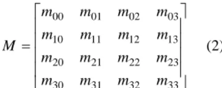
= 33 32 31 30 23 22 21 20 13 12 11 10 03 02 01 00 m m m m m m m m m m m m m m m m M (2)
One can multiply the Stokes vector 𝑆𝑆⃗𝑖𝑖𝑖𝑖, describing the polarization state of incident light, by a material’s Mueller matrix M to calculate the Stokers vector 𝑆𝑆⃗𝑜𝑜𝑜𝑜𝑜𝑜 describing the polarization state of the reflected (or transmitted) light, as follows:
out in
S S
MC = C (3)
The Mueller matrix M can be converted to a covariance matrix Σ (not to be confused with the symbol for summation) as follows [28]:
∑∑
= = ⊗ = Σ 4 0 4 0 2 1 i j j i ij m σ σ (4)where
⊗
denotes the Kronecker product of matrices, and σi are thePauli matrices defined as:
− = = − = = 0 0 0 1 1 0 1 0 0 1 1 0 0 1 4 3 2 1 i i σ σ σ σ (5)
The covariance matrix Σ can also be expressed as: 1 − Λ =
Σ V V (6)
where Λ is a 4 x 4 diagonal matrix containing the four eigenvalues λi of Σ, and V is the corresponding matrix of unitary column
eigenvectors vi. The covariance matrix of any physically realizable
(i.e., valid) Mueller matrix is guaranteed to be a positive semi-definite Hermitian (PSDH) matrix, which means that all four of Σ’s eigenvalues are positive or zero. Thus, a condition for an arbitrary 4 x 4 real matrix to be a physically realizable (i.e. valid) Mueller matrix is that the eigenvalues of its associated covariance matrix meet this criterion [28, 29]:
3 , 2 , 1 , 0 0 = ≥ i i λ (7)
B. Mueller Matrix Decomposition
A material’s Mueller matrix can be decomposed to quantify its underlying polarimetric behavior. Any given material can exhibit a combination of three fundamental polarimetric behaviors [20]. Diattenuation is the preferential reflection (or transmittance) of certain polarization states over others. Retardance is the introduction of a phase shift between certain polarization states, by retarding one of their phases relative to the other. Depolarization is the conversion of polarized light into partially polarized or unpolarized light.
0018-9251 (c) 2016 IEEE. Translations and content mining are permitted for academic research only. Personal use is also permitted, but republication/redistribution requires IEEE permission. See Lu and Chipman [30] describe the mathematics for decomposing
a Mueller matrix into the product of three matrices corresponding to these fundamental behaviors:
D RM
M M
M = D (8)
where 𝑀𝑀𝐷𝐷, 𝑀𝑀𝑅𝑅, and 𝑀𝑀𝛥𝛥 are the 4 x 4 diattenuation, retardance, and depolarization factors, respectively. The general form of each matrix in Eq. 8 is:
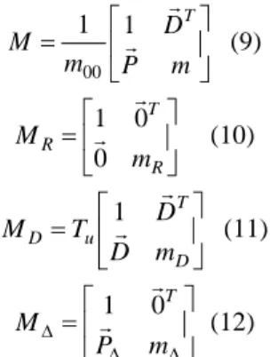
= m P D m M T C C 1 1 00 (9) = R T R m M 0 0 1 C C (10) = D T u D m D D T M C C 1 (11) = D D D m P M T C C 0 1 (12)
where T is the symbol for transposing a vector, 𝑇𝑇𝑜𝑜= 𝑚𝑚00−1 is the reflectivity (or transmittivity) for unpolarized light, 𝐷𝐷��⃗ is the diattenuation vector, 𝑃𝑃�⃗ and 𝑃𝑃�⃗∆ are the polarizance vectors of M and 𝑀𝑀𝛥𝛥 , respectively, 𝑚𝑚, 𝑚𝑚𝐷𝐷, 𝑚𝑚𝑅𝑅, and 𝑚𝑚𝛥𝛥 are the 3 x 3 sub-matrices of their respective parent matrices, and 0�⃗ is a 3 x 1 vector of zeros. Since matrix multiplication is not commutative, a Mueller matrix could also be decomposed with the factors permutated in five other possible sequences (e.g., 𝑀𝑀 = 𝑀𝑀𝑅𝑅𝑀𝑀𝐷𝐷𝑀𝑀∆), which can, in some cases, lead to a different interpretation of the material’s behavior. We have restricted our analysis to the sequence in Eq. 8, since it is readily mathematically obtainable and has clear separation of the depolarizing (𝑀𝑀𝛥𝛥) and nondepolarizing (𝑀𝑀𝑅𝑅𝑀𝑀𝐷𝐷) contributions [30]. The decomposition reveals an array of polarimetric properties describing the material’s polarimetric behavior.
C. Mueller Matrix Decomposition
This paper highlights three specific polarimetric properties computed directly from the decomposed Mueller matrix. The first property is diattenuation (D), which is a dimensionless number (range 0 to 1) indicating how strongly the material reflects (or transmits) some polarization states relative to others [30]. A perfect diattenuator (e.g., an ideal linear polarizer) has a diattenuation of D = 1. Diattenuation is simply the magnitude of its diattenuation vector:
D D= C (13)
The second property considered in this paper is retardance (R), which is the relative phase shift, in units of radians or degrees (range 0 to 180º), induced by the material onto its orthogonal eigenpolarizations [30]. A half-wave and quarter-wave plate have retardances of R = 180º and R = 90 º, respectively. The retardance is related to the trace (tr) of the retardance factor 𝑀𝑀𝑅𝑅 as follows:
− = − 1 2 ) ( tr cos 1 MR R (14)
The third property of interest here is depolarization power (Δ), which is a dimensionless number (range 0 to 1) indicating how strongly the material depolarizes incident light [30]. An ideal depolarizer has a depolarization power of Δ = 1. The depolarization power of a material is related to the three eigenvalues 𝜆𝜆𝑖𝑖𝛥𝛥 of the sub-matrix 𝑚𝑚𝛥𝛥 inside the depolarization factor 𝑀𝑀𝛥𝛥 as follows:
3 1 0 1 2 D D D + + − = D
λ
λ
λ
(15)Many other polarimetric properties are also obtainable from the elements of the Mueller matrix and its decomposition [22, 23, 30]. For example, the polarizance 𝑃𝑃 = |𝑃𝑃�⃗| (range 0 to 1) describes how strongly the material converts unpolarized light into polarized light. All properties are potentially exploitable as a means of characterizing and identifying the material being measured. We chose to focus on the properties of diattenuation (D), retardance (R), and depolarization power (Δ) since they quantify the three fundamental polarimetric behaviors.
Figure 2 Depiction of active polarimetry with Mueller calculus notation D. Mueller Matrix Estimation
Polarimetry makes it possible to partially or completely determine a material or object’s Mueller matrix and associated polarimetric properties. Whether polarimetry is done passively or actively, the governing mathematics, as depicted in Figure 2, are the same. If 𝑆𝑆⃗𝑇𝑇𝑇𝑇 is the Stokes vector of the light incident upon the material (whether from the sun or a laser), M is the Mueller matrix of the material being measured, and 𝑀𝑀𝑅𝑅𝑇𝑇 is the Mueller matrix of the polarization analyzers placed in front of the detector, then the Stokes vector 𝑆𝑆⃗𝑅𝑅𝑇𝑇 of the light reaching the detector is given by applying Eq. 3 twice sequentially:
Tx Rx Rx S M M SC = C (16)
In our notation, 𝑆𝑆⃗𝑇𝑇𝑇𝑇 is the Stokes vector of Tx-polarized (e.g., H-polarized, or horizontally polarized) light that is “transmitted” (Tx) or sent to the material, while 𝑀𝑀𝑅𝑅𝑇𝑇 is a Mueller matrix that “receives” (Rx) or passes the Rx-polarized component of the reflected light. Meanwhile, the Stokes vector 𝑆𝑆⃗𝑅𝑅𝑇𝑇 of the light that ultimately reaches the detector is actually inconsequential, since according to Eq. 1, the intensity 𝐼𝐼𝑇𝑇𝑇𝑇𝑅𝑅𝑇𝑇measured by the detector is equal to the first element 𝑠𝑠0𝑅𝑅𝑇𝑇 of 𝑆𝑆⃗𝑅𝑅𝑇𝑇 (i.e., independent of polarization):
∑ ∑
= ==
=
3 0 3 0 0 0 i j ij Tx j Rx i Rx TxRxs
m
s
m
I
(17)where 𝑚𝑚0𝑖𝑖𝑅𝑅𝑇𝑇is element i of the first row of 𝑀𝑀𝑅𝑅𝑇𝑇, 𝑠𝑠𝑗𝑗𝑇𝑇𝑇𝑇 is element j of 𝑆𝑆⃗𝑇𝑇𝑇𝑇, and mij is element (i, j) of M. If the 4 x 4 matrix M is reshaped
to be a 16 x 1 vector 𝑀𝑀��⃗, then Eq. 18 can be rewritten as a dot product:
M
h
I
TxRx TxRxC
C
=
(18)where the vectors 𝑀𝑀��⃗ and ℎ�⃗𝑇𝑇𝑇𝑇𝑅𝑅𝑇𝑇 are constructed as follows:
[
]
T m m m M = 00 10 ... 33 C (19)[
Rx Tx Rx Tx Rx Tx]
TxRxm
s
m
s
m
s
h
=
00 0 01 0...
33 3C
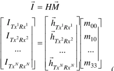
(20) Eq. 19 is the crux of polarimetry. By measuring 𝐼𝐼𝑇𝑇𝑇𝑇𝑛𝑛𝑅𝑅𝑇𝑇𝑛𝑛 for N different Tx-Rx pairs, one can construct a system of N equations, each in the form of Eq. 19:0018-9251 (c) 2016 IEEE. Translations and content mining are permitted for academic research only. Personal use is also permitted, but republication/redistribution requires IEEE permission. See = = 33 10 00 ... ... ... 2 2 1 1 2 2 1 1 m m m h h h I I I M H I N N N N Rx Tx Rx Tx Rx Tx Rx Tx Rx Tx Rx Tx C C C C C (21) where the vectors 𝐼𝐼⃗ and matrix H are concatenations of the N measured intensities 𝐼𝐼𝑇𝑇𝑇𝑇𝑛𝑛𝑅𝑅𝑇𝑇𝑛𝑛 and associated vectors ℎ�⃗𝑇𝑇𝑇𝑇𝑛𝑛𝑅𝑅𝑇𝑇𝑛𝑛, respectively. Assuming a determined system (N linear independent equations, N unknowns), Eq. 22 can be solved as follows:
I
H
M
C
=
−1
(22)Depending on which elements of H are non-zero, the measured intensities 𝐼𝐼⃗ may be linear functions of some or all of the unknown Mueller matrix elements mij. With active polarimetry, one has
individual control over both Tx and Rx, so measured intensities ITxRx are generally functions of all 16 elements of M. Thus, by
making N = 16 different Tx-Rx measurements, active polarimetry can solve for the entire Mueller matrix. If more than 16 measurements are made, the over-determined systems of equations can be solved with a least-squares estimator [31].
E. Treatment of Experimental Mueller Matrices
In practice, Mueller matrix estimation is complicated by measurement errors. A noisy experimental Mueller matrix is unlikely to be physically realizable (Eq. 7), such that decomposition will yield nonsensical results. Cloude [28] provides a method for filtering an experimental Mueller matrix that does not satisfy Eq. 7 due to having a covariance matrix Σ (Eq. 4) with negative eigenvalues. Specifically, one can change all the negative eigenvalues to zero, calculate the new covariance matrix using Eq. 6, and calculate the associated Mueller matrix using the inverse of Eq. 4. The “filtered” Mueller matrix is now, in some sense, the closest physically realizable Mueller matrix to the original noisy one, and can be legitimately decomposed as desired. The eigenvalue ratio γ of the largest (in magnitude) negative eigenvalue (of the original Σ) to the largest positive one can be calculated in decibels as follows: ⋅ = λ λ γ positive max | negative max | log 10 10 (23) The ratio γ is a measure of how close the original experimental Mueller matrix was to being physically realizable. Negative values of γ are expected, indicating that the negative eigenvalues are smaller (in magnitude) than the positive ones. Values of γ < -10 dB generally indicate experimental Mueller matrices that are very close to being physically realizable [28, 32].
F. Polarimetric BRDF
When performing polarimetry on a material or object, the apparent Mueller matrix will depend on the illumination and viewing geometry, as quantified by the Bidirectional Reflectance Distribution Function (BRDF) [33, 34]. Nominally, a material’s BRDF(θi,ϕi,θs,ϕs), expressed in inverse steradians (sr-1), is a function
of the zenith angle θi (0 to 90°) and azimuth angle ϕi (-180 to 180°)
of the incident beam, as well as those of the direction of scatter (θs
and ϕs). More specifically, a material’s BRDF also varies as a
function of polarization, such that one would measure a different
amount of scatter depending on the polarization state (Tx) of the incident light and the polarization component (Rx) of the reflected light that is passed through to the detector. Therefore, a material’s polarimetric (or polarization-dependent) BRDF, written BRDF(θi,ϕi,θs,ϕs,Tx,Rx), can be computed from its
geometry-dependent Mueller matrix, written M(θi,ϕi,θs,ϕs), using Eq. 17 as
follows: Tx s s i i Rx row s s i i
Tx
Rx
M
M
S
BRDF
(
θ
,
φ
,
θ
,
φ
,
,
)
=
0(
θ
,
φ
,
θ
,
φ
)
C
(24)where 𝑀𝑀𝑅𝑅𝑇𝑇 and 𝑆𝑆⃗𝑇𝑇𝑇𝑇 are unit-less, but M(θi,ϕi,θs,ϕs) is given units
of sr-1 [20]. By analogy with Eq. 22, one can make N = 16 different Tx-Rx measurements at geometry (θi,ϕi,θs,ϕs) to compute the
Mueller matrix M(θi,ϕi,θs,ϕs) at that geometry. We made these
measurements using a bench-top polarimeter to investigate the polarimetric behavior of spacecraft materials.
Figure 3 Diagram of bench-top polarimeter
III. EXPERIMENTAL SETUP AND PROCEDURE We implemented a bench-top polarimeter (Figure 3) to measure the polarimetric BRDF of material samples. The polarimeter uses a continuous-wave (CW) laser (Spectra-Physics® model Excelsior 1064-800) with a wavelength of λ = 1064 nm. Several ground-based laser radars used for space surveillance also operate at 1064 nm using solid-state Nd:YAG lasers [8, 35]. The raw laser beam., which is horizontally polarized, passes through a half-wave (λ/2) plate and quarter-wave (λ/4) plate, which are independently rotated (using Newport® PR50CC rotation stages) to control the polarization state (Tx) of the transmitted beam (i.e., 𝑆𝑆⃗𝑇𝑇𝑇𝑇 in Eq. 17). The beam (3 mm diameter) then encounters the material being measured. The reflected light is measured by two silicon detectors (Thorlabs model PDA36A), one for bistatic measurements and one for quasi-monostatic measurements (where the laser and detector are separated by < 1º). Each detector is preceded by a λ/4 plate and λ/2 plate, which are independently rotated (Newport®PR50CC) to control the received polarization state (Rx) (i.e., 𝑀𝑀𝑅𝑅𝑇𝑇 in Eq. 17) and a fixed linear polarizer. Lenses and irises are used to give a
field-of-0018-9251 (c) 2016 IEEE. Translations and content mining are permitted for academic research only. Personal use is also permitted, but republication/redistribution requires IEEE permission. See view of 1 cm (on the material) and the subtended solid angle (Ω),
respectively. To record a measurement, the laser is chopped at a frequency of 100 Hz and the detector’s analog output is acquired using a lock-in amplifier (Princeton Applied Research Model 5209).
Rotation stages (Newport®RV120CCHL) are additionally used to control the illumination and viewing geometry. The material is rotated (in the plane of the diagram) to achieve arbitrary incident zenith angles (θi) for a fixed azimuth angle (ϕi). For monostatic
angular scans, only the material is rotated. For bistatic angular scans for a fixed θi, the bistatic receiver assembly is rotated about the laser
spot (on the material) to achieve arbitrary scatter zenith angles (θs)
in the plane of incidence. All rotation stages are motorized and data collection is automated using Matlab®.
Figure 4 Hypothetical polarimetric BRDFs (i.e., in-plane bistatic scans)
Figure 5 Hypothetical polarimetric MRDFs (i.e., monostatic scans) Since our bench-top polarimeter measures a material’s bistatic or monostatic BRDF as functions of zenith angles at fixed azimuth angles, we have adopted a simplified nomenclature and notation for the polarimetric BRDF. Henceforth, the term “BRDF” will refer only to an in-plane bistatic scan (Figure 4), written mathematically as BRDF(θi,θ,Tx,Rx) where the azimuth arguments have been removed and the scatter zenith angle θs has been replaced by θ (-90º to (-90º). The backward, forward, and specular scatter regimes are defined by θ < 0, θ > 0, and θ ≈ θi, respectively. Meanwhile, the term ”MRDF” (“M” for monostatic) will refer to a monostatic scan (Figure 5), written mathematically as MRDF(θ,Tx,Rx) where the incident and scatter zenith angles are equal, by definition, and represented by θ (0 to 90º). Here, the specular and diffuse regimes are defined by θ ≈ 0º and θ > 0º, respectively.
TABLE 1INTENSITY MEASUREMENTS FOR 16TX-RX PAIRS Transmit Polarization (Tx) H V +45 RC Receive Polarization (Rx) H IHH IVH I+45H IRCH V IHV IVV I+45V IRCV +45 IH+45 IV+45 I+45+45 IRC+45 RC IHRC IVRC I+45RC IRCRC
At a given illumination and viewing geometry, the intensity 𝐼𝐼𝑇𝑇𝑇𝑇𝑅𝑅𝑇𝑇 of the scattered light is measured for each of the 16 Tx-Rx polarization pairs in Table 1, where horizontal, vertical, +45°, and right-hand circular polarizations have been abbreviated by H, V, +45, and RC, respectively. For simplicity, the intensity for each polarization pair is sequentially measured and immediately recorded, as opposed to a scheme with dual rotating retarders (DRR) and Fourier analysis [36]. The polarimetric BRDFs (in-plane bistatic scan) and MRDFs (i.e., monostatic scan) are then calculated as follows [33]:
θ
θ
θ
θ
θ
cos ) , , ( cos ) , , , ( 0 0 Ω = Ω = I I Rx Tx MRDF I I Rx Tx BRDF TxRx TxRx i (25)where I0 is the intensity of the incident beam (which is the same for
all Tx) and Ω = 500 μsr is the solid angle subtended by the iris. The BRDF or MRDF value is a function of the measured variables I, I0,
Ω, and θ, which are uncorrelated Therefore, the variance 𝜎𝜎𝑇𝑇𝑇𝑇𝑅𝑅𝑇𝑇2 on the estimated BRDF at polarization pair TxRx is the sum of the variances of the measured variables weighted by the squares of the partial derivatives of BRDF [37]: 2 2 2 2 2 2 0 2 2 2 0 θ
σ
θ
σ
σ
σ
σ
∂
∂
+
Ω
∂
∂
+
∂
∂
+
∂
∂
=
ΩBRDF
BRDF
I
BRDF
I
BRDF
I I TxRx (26)where 𝜎𝜎𝐼𝐼2, 𝜎𝜎𝐼𝐼02, 𝜎𝜎𝛺𝛺2, and 𝜎𝜎𝜃𝜃2 are variances on the measured values of I, I0, Ω, and θ, respectively.
Each of the 16 intensity measurements (Table 1) contributes a linearly independent equation in the form of Eq. 19, allowing us to solve for the geometry-dependent Mueller matrix using Eq. 23. Each estimate Mueller matrix is filtered to ensure physical realizability. We then decompose each filtered Mueller matrix (in the form of Eq. 8) to calculate its polarimetric properties as a function of the illumination and viewing angles.
Figure 6 Measured vs. reference BRDF of Spectraflect® at θ
0018-9251 (c) 2016 IEEE. Translations and content mining are permitted for academic research only. Personal use is also permitted, but republication/redistribution requires IEEE permission. See A. Validation
We validated the bench-top polarimeter in terms of its ability to measure (1) a reference sample with a known BRDF and (2) some common optical elements with known Mueller matrices. First, we measured the BRDF of a sample of Spectraflect®, a coating that is approximately Lambertian over the wavelength range from 350 to 2400 nm [38]. The manufacturer (Labsphere®) provided reference data on Spectraflect’s in-plane BRDF for λ = 633 nm, incident angle θi = 30°, a Tx polarization of H (i.e., horizontally or “p” polarized), and an Rx polarization of U (or unpolarized, i.e., there was no polarization analyzer in front of the detector). For comparison, we measured the in-plane BRDF of Spectraflect® for λ = 1064 nm, θi = 30°, and Tx-Rx polarizations of HH and HV (separately). Following Pickering’s method [39], the sum of our measured BRDFs at HH and HV should be equivalent to the reference BRDF at HU. Spectral differences between our measurement (1064 nm) and the reference (633 nm) are expected to be negligible [38]. As plotted in Figure 6, our measurement matches the reference data well within the error bounds of the measurement at almost every angle. This result validated our system’s ability to accurately measure BRDF curves. Note that Spectraflect® has an approximately constant BRDF of π-1≈ 0.32, as expected for a Lambertian surface [33]. Note also that there are no data points for angles (θ) from -40º to -20º, because the bistatic receiver assembly would block the laser before hitting the material sample. These data gaps exist in all of our bistatic scans.
We also measured several common (transmissive) optical elements, where each element was illuminated at normal incidence and the detector assembly was positioned directly on the other side of the element. From the 16 prescribed measurements (Table 1), we calculated the Mueller matrix of each optical element. Despite measurement noise, all estimated Mueller matrices had associated eigenvalue ratios (Eq. 24) of γ < -18 dB, indicating that they were all extremely close to physically realizable (i.e., valid) matrices. We then filtered and decomposed (Eq. 8) each estimated Mueller matrix and computed its polarimetric properties, including diattenuation (D, Eq. 14), retardance (R, Eq. 15), and depolarization power (Δ, Eq. 16). ERROR!REFERENCE SOURCE NOT FOUND.TABLE 2 compares the experimental properties with the theoretical ones for each optical element, as well as for Spectraflect®. All the theoretical D’s and Δ’s are 0 or 1, and all the theoretical R’s are 0º, 90º, or 180º. For the optical elements, the experimental D’s and Δ’s are within 0.01 of their respective theoretical values, and the experimental R’s are within 4º. As expected, the Spectraflect® sample appeared highly depolarizing (Δ = 0.93), but we did not have a reference value for direct comparison. Previous studies [17] achieved errors comparable to ours when measuring theoretical
targets. These results showed that we can use our bench-top polarimeter (Figure 3) to accurately estimate Mueller matrices, decompose them, and compute their polarimetric properties.
B. Measurement of Spacecraft Materials
We used the bench-top polarimeter to measure the polarimetric BRDFs (i.e., in-plane bistatic scans) and MRDFs (i.e., monostatic scans) of several materials and coatings commonly found on man-made satellites and debris [40], including glossy white paint (Aeroglaze® A276), matte black paint (Aeroglaze® Z306), black Kapton®, silver Teflon®, aluminum alloy (sheet of 6061-T6), and titanium alloy (6Al-4V). For each spacecraft material, we measured the BRDFs for incident angles of θi = 15, 30, 45, 60 and 75° and scatter angles θ from -80º to 80º with 1° resolution around the expected specular (±10°) and 5° resolution elsewhere. We also measured the MRDFs of a subset of the materials, namely glossy white paint, silver Teflon®, aluminum alloy, and titanium, at incident/scatter angles θ from 0 to 85º (at higher angles the spot size became elongated beyond the edge of the material samples) with 0.1° resolution around the expected specular (±10°) and 1° resolution elsewhere. BRDFs and MRDFs were measured for the 16 prescribed Tx-Rx polarization pairs (Table 1), allowing us to calculate each material’s Mueller matrix and polarimetric properties as functions of the illumination and viewing angles.
IV. EXPERIMENTAL RESULTS
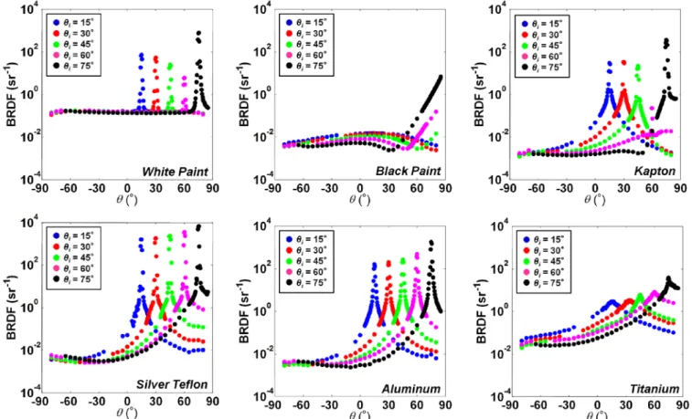
Here we present the results of our experiments on the spacecraft materials introduced above. We first consider the BRDFs and MRDFs measured for each spacecraft material for a single polarization pair. Figure 8 shows each spacecraft material’s MRDF measured at polarization pair HH, while Figure 7 shows the BRDFs (at HH) measured for several incident angles θi. All
materials have a dominant specular component at θ ≈ θi, with the
exception of the matte black paint, which is mostly diffuse but with significantly increased forward scatter for high incident angles. Using the 16 polarimetric BRDFs and MRDFs measured for each material, we computed the materials’ Mueller matrices and polarimetric properties as functions of angle, i.e., M(θi,θ) for bistatic
and M(θ) for monostatic). No attempt was made to smooth the measured polarimetric BRDFs or MRDFs with a low-pass filter or other smoothing method. All estimated Mueller matrices had associated eigenvalue ratios (Eq. 24) of γ < -10 dB, indicating that they were very close to physically realizable (i.e., valid) matrices.
TABLE 2COMPARISON OF THEORETICAL AND EXPERIMENTAL POLARIMETRIC PROPERTIES OF REFERENCE SAMPLES Reference
Sample
D R Δ
Theory Measurement Theory Measurement Theory Measurement
Air 0 0.03 0º 1.7 0 0.01
Polarizer 1 1.00 0º 2.2 0 0.00
λ/2 Plate 0 0.03 180º 178.4 0 0.01
0018-9251 (c) 2016 IEEE. Translations and content mining are permitted for academic research only. Personal use is also permitted, but republication/redistribution requires IEEE permission. See Figure 7 Measured BRDFs (i.e., in-plane bistatic scans) of spacecraft materials at polarization pair HH
Figure 8 Measured MRDFs (i.e., monostatic scans) of spacecraft materials at polarization pair HH
Figure 9 plots the materials’ bistatic polarimetric properties calculated from their measured BRDFs (i.e., in-plane bistatic scans). Each material’s diattenuation (D), retardance (R), and depolarization power (Δ) is plotted as functions of θ for all θi. The
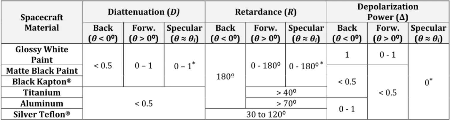
plots reveal some notable trends and value ranges in these bistatic polarimetric properties, as summarized approximately in TABLE 3, according to the direction of scatter: backward (θ < 0), forward (θ > 0), and specular (θ ≈ θi).
Referring to TABLE 3, all materials exhibited mostly low diattenuation (D < 0.5) in the back scatter direction. However, in the forward scatter direction (including the specular), the metallic surfaces (i.e., titanium, aluminum, and silver Teflon®) continued exhibiting D < 0.5, while the two paints and Kapton® had the full range of diattenuaton (D = 0 to 1). In terms of retardance, the silver Teflon® uniquely exhibited a finite range (R = 30 to 120º) in all
scatter directions, while all other materials acted as mirrors (R = 180º) in the back scatter direction and had the full range of behavior (R = 0 to 180º) in the forward scatter direction. Finally, in terms of depolarization power, the glossy white paint was a nearly perfect depolarizer (Δ ≈ 1) in the back-scatter direction, but sharply lost depolarization power (Δ = 0) at specular reflection. All other materials were mostly weak depolarizers (Δ < 0.5) in all directions, except that silver Teflon® and aluminum exhibit moderately high depolarization power (0.5 < Δ < 0.8) in the back scatter direction. Figure 10 plots the materials’ monostatic polarimetric properties (D, R, and Δ) calculated from their measured MRDFs. (i.e., monostatic scans). TABLE 4 summarizes the approximate trends in the materials’ monostatic polarimetric properties with respect to the specular (θ ≈ 0º) and diffuse (θ > 0º) regimes. All the materials exhibited very little diattenuation (D < 0.1) around the specular point, with the exception of Kapton®, which showed slightly higher value of D = 0.2. Diattenuation increased monotonically into the diffuse region for all materials, achieving values as high as D = 0.8 for black paint and Kapton®, D = 0.4 for aluminum, and D = 0.2 for all other materials. In terms of retardance, all the materials were mirror-like (R = 180°) at all angles, except for silver Teflon®, which had a distinct retardance of R = 115º at the specular point and a range of values elsewhere, and aluminum, which had a retardance of R = 180° at the specular point and decreasing values into the diffuse region. The peculiar retardance of silver Teflon® also appeared in its bistatic behavior. Finally, in terms of depolarization power, all the materials were nondepolarizing (Δ = 0) at the specular point and had increasing depolarizing power into the diffuse region. The white paint sample actually had a relatively constant depolarization power of Δ = 0.7 to 0.9 in the diffuse region.
0018-9251 (c) 2016 IEEE. Translations and content mining are permitted for academic research only. Personal use is also permitted, but republication/redistribution requires IEEE permission. See Overall, the trends identified in TABLE 3 and TABLE 4 follow
expected patterns and agree with previous studies [13, 17, 18]. At specular points, metallic surfaces (i.e., aluminum and titanium) exhibited mirror-like behavior (D = 0, R = 180º, Δ = 0), while paints and thin films (e.g., Kapton®) were diattenuating (D > 0) as expected from Fresnel reflection. The distinguishing behavior of materials at the specular points is particularly important, since the polarimetric signatures of space objects will likely be dominated by the specular reflections from their smooth surfaces. Meanwhile, in the diffuse regime, all the studied materials tended to be more depolarizing, since diffuse reflections tend to be depolarized by surface roughness [20, 33]. Silver Teflon® followed the trends of a metallic surface, with the exception of its distinctly finite band of retardance values in the specular and diffuse regions.
V. CONCLUSION
Our objective is to assess the utility and feasibility of polarimetric laser radars for characterizing space debris objects. We have measured polarimetric BRDFs of common space materials in both bistatic and monostatic geometries, and estimated their Mueller matrices and associated polarimetric properties as functions of illumination and viewing angles. Our findings were consistent with previous research in that the materials exhibited notable trends in their geometry-dependent polarimetric behavior (TABLE 3 and TABLE 4), especially mirror-like behavior at specular points and increasing depolarization power when transitioning to the diffuse regime. In addition, we demonstrated some especially unique behaviors, particularly the retardance of silver Teflon®. Our work contributes to the small, but growing database of polarimetric measurements of spacecraft materials and expands on previous studies by increasing the range and resolution of angles, the number of materials characterized with the same experiment, and the number of polarization metrics assessed.
Outstanding research questions need to be addressed before a polarimetric laser radar for space surveillance can be realized in the future. In terms of phenomenology, although we have measured the polarimetric BRDFs of “coupon” samples of individual spacecraft materials, we have not yet considered the signature of a non-resolved (i.e., in angle) space objects, whose surface compositions may include a single material, multiple separate materials, or an intimate mixture of materials [41]. In future work, we plan to simulate these signatures in software by modeling the outer hull of a space object and predicting the combined signal
returned by its surface facets using the polarimetric BRDFs measured in the current study. Error analysis will be needed to determine whether differences between object signatures are statistically significant for debris identification purposes. Though tedious, error bounds may be computed by propagating the errors on the measured BRDFs through the processing chain of Mueller matrix estimation and decomposition [42].
Other challenging aspects of active polarimetry for space surveillance include the effects of object tumbling, space weather, and atmospherics effects. Space debris can be tumbling at rates from 0.1s to 10s of º/sec [43], which may blur an object’s signature relative to a stationary case. Nevertheless, a polarimetric laser radar could possibly mitigate the effect of tumbling by synchronizing its polarization switching and/or data analysis with the object’s rotational frequency, as determined by an auxiliary passive optical telescope [44]. If accounted for, tumbling may actually provide additional angular diversity that could improve discrimination capabilities. The surfaces of space objects and debris will also degrade over time due to space weather [45], which may alter their reflectivity, surface roughness, and polarimetric properties. Future experiments could include measurements of space-aged materials (e.g., from the Materials International Space Station Experiment [MISSE] campaign [45]) to help anticipate the polarimetric effects of space erosion. Changes in the polarimetric signatures of space objects may also provide a useful means of remotely monitoring the amount of space erosion that has occurred on an on-orbit object. A ground-based polarimetric laser radar would also suffer from the attenuation and polarization effects of the atmosphere, which would need to be accounted for or mitigated operationally, such as by pointing overhead through minimal atmosphere. These practical operational considerations require investigation in future work. Algorithms will also be needed to categorize and discriminate between the polarimetric signatures of space debris [25, 29]. The optimal classification scheme may need to fuse polarimetric, spectral, RF, and orbital features [46]. A robust classification scheme will rely on an accurate understanding of polarimetric phenomenology from laboratory measurements as explored in this paper. If further laboratory experiments can establish that a debris fragment’s polarimetric signature is robustly exploitable, then a field test may be appropriate. An existing laser radar system could then conceivably be augmented to perform active polarimetry on orbiting space debris to validate the concept of operation in the field.
0018-9251 (c) 2016 IEEE. Translations and content mining are permitted for academic research only. Personal use is also permitted, but republication/redistribution requires IEEE permission. See Figure 9 Measured bistatic polarimetric properties of spacecraft materials
0018-9251 (c) 2016 IEEE. Translations and content mining are permitted for academic research only. Personal use is also permitted, but republication/redistribution requires IEEE permission. See
TABLE 3TRENDS IN BISTATIC POLARIMETRIC PROPERTIES
Spacecraft Material
Diattenuation (D) Retardance (R) Depolarization Power (Δ) Back (θ < 0º) (θ > 0º) Forw. Specular (θ ≈ θi) Back (θ < 0º) (θ > 0º) Forw. Specular (θ ≈ θi) Back (θ < 0º) (θ > 0º) Forw. Specular (θ ≈ θi) Glossy White Paint < 0.5 0 – 1 0 – 1* 180º 0 - 180º 0 - 180º * 1 0 - 1 0* Matte Black Paint
< 0.5 < 0.5 Black Kapton® Titanium < 0.5 > 40º Aluminum > 70º 0 - 1 Silver Teflon® 30 to 120º
* Specular trends do not apply to matte black paint
Figure 10 Measured monostatic polarimetric properties of spacecraft materials
TABLE 4TRENDS IN MONOSTATIC POLARIMETRIC PROPERTIES
Spacecraft Material
Diattenuation (D) Retardance (R) Depolarization Power (Δ) Diffuse (θ > 0º) Specular (θ ≈ 0º) Diffuse (θ > 0º) Specular (θ ≈ 0º) Diffuse (θ > 0º) Specular (θ ≈ 0º) White Paint < 0.4 < 0.1 180° > 150° 0.7 - 0.9 0 Black Paint < 0.8 180° < 0.3 Kapton® 0.2 > 150° < 0.5 Silver Teflon® < 0.3 < 0.1 0 - 180° 115° < 0.9 Aluminum < 0.4 180° < 0.7 Titanium < 0.2 180° < 0.3 VI. BIBLIOGRAPHY
[1] Inter-Agency Space Debris Coordination Committee, Stability of the Future LEO Environment, 2013. [2] N. J. Johnson and D. S. McKnight, Artificial Space
Debris, Malabar, FL: Krieger Publishing Company, 1991. [3] Inter-Agency Space Debris Coordination Committee,
Space Debris Mitigation Guidelines, 2007.
[4] D. J. Kessler and B. G. Cour-Palais, "Collision frequency of artificial satellites: the creation of a debris belt," Journal of Geophysical Research, vol. 83, no. A6, pp. 2637-2646, 1978.
[5] J. C. Liou, “An active debris removal parametric study for LEO environment remediation,” Advances in Space Research, vol. 47, pp. 1865-1876, 2011.
[6] N. N. Smirnov, Ed., Space Debris: Hazard Evaluation
and Mitigation, New York: Taylor and Francis, 2002. [7] J. W. Campbell, "Using lasers in space," 2000.
[8] J. D. Eastment, D. N. Ladd and C. J. Walden, "Technical description of radar and optical sensors contributing to joint UK-Australian satellite tracking, data fusion and cueing experiment," in Advanced Maui Optical and Space Surveillance Technologies Conference, Wailea, HI, 2014.
[9] G. C. Giakos, R. H. Picard and P. D. Dao,
"Superresolution multispectral imaging polarimetric space surveillance LADAR sensor design architectures," in Remote Sensing, 2008.
[10] J. Sang, J. C. Bennett and C. Smith, "Experimental results of debris orbit predictions using space tracking data from Mt. Stromlo," Acta Astronautica, vol. 102, pp. 258-268, 2014.
[11] Z.-P. Zhang, F.-M. Yang, H.-F. Zhang, Z.-B. Wu, J.-P. Chen, P. Li and W.-D. Meng, "The use of laser ranging to measure space debris," Research in Astronomic and Astrophysics.
0018-9251 (c) 2016 IEEE. Translations and content mining are permitted for academic research only. Personal use is also permitted, but republication/redistribution requires IEEE permission. See [12] B. Greene, G. Yuo and M. Christ, "Laser tracking of
space debris," in 13th International Workshop n Laser Ranging, Washington, D.C., 2002.
[13] G. C. Giakos, R. H. Picard, P. D. Dao and P. Crabtree, “Object detection and characterization by monostatic ladar bidirectional reflectance distribution function (BRDF) using polarimetric discriminants,” Proc. SPIE, Electro-Optical Remote Sensing, Photonic Technologies, and Applications III, vol. 7482, 2009.
[14] N. L. Seldomridge, J. A. Shaw and K. S. Repasky, “Dual-polarization lidar using a liquid crystal variable retarder,” Optical Engineering, vol. 45, no. 10, p. 106202, 2006. [15] M. H. Smith, “Optimization of a dual-rotating-retarder
Mueller matrix polariemter,” Applied Optics, vol. 41, no. 13, pp. 2488-2493, 2002.
[16] G. C. Giakos, R. H. Picard, P. D. Dao, P. N. Crabtree and P. J. McNicholl, “Polarimetric Wavelet Phenomenology of Space Materials,” in IEEE International Conference on Imaging Systems and Techniques, Batu Ferringhi, Malaysia, 2011.
[17] J. Peterman, “Design of a Fully Automated Polarimetric Imaging System for Remote Characterization of Space Materials,” in The Univerity of Akron, MS Thesis, 2012. [18] M. Reddy, “Advanced Object Characterization and
Monitoring Techniques Using Polarimetric Imaging,” in The University of Akron, MS Thesis, 2009.
[19] K. Rochford, "Polarization and Polarimetry," National Institute of Standards and Technology.
[20] J. R. Schott, Fundamentals of Polarimetric Remote Sensing, Bellingham, WA: SPIE Press, 2009. [21] J. S. Tyo, D. L. Goldstein, D. B. Chenault and J. A.
Shaw, “Review of passive imaging polarimetry for remote,” Applied Optics, vol. 45, no. 22, pp. 5453-5469, 2006.
[22] J. L. Pezzaniti and R. A. Chipman, "Mueller matrix imaging polarimetry," Optical Engineering, vol. 34, no. 6, 1995.
[23] P. Refregier, F. Goudail and N. Roux, "Estimation of the degree of polarization in active coherent imagery by using the natural representation," Journal of the Optical Society of America A, vol. 21, no. 12, 2004.
[24] S. Breugnot and P. Clemenceau, “Modeling and performance of polarimetric active imager at 806nm,” Optical Engineering, vol. 30, no. 10, pp. 2681-2688, 2000.
[25] C. S. Chun and F. A. Sadjadi, “Polarimetric laser radar target classification,” Optics Letters, vol. 30, no. 14, pp. 1806-1808, 2005.
[26] J. S. Baba, J.-R. Chung, A. H. DeLaughter, B. D. Cameron and G. L. Cote, “Development and calibration of a m automated Mueller matrix polarization imaging system,” Journal of Biomedical Optics, vol. 7, no. 3, pp. 341-349, 2002.
[27] E. Hecht, Optics, Boston: Pearson, 2002.
[28] S. R. Cloude, "Conditions for the physical realisability of
matrix operatrors in polarimetry," in SPIE Polarization Considerations for Optical Systems II, 1989.
[29] F. Boulvert, G. Le Brun, B. Le Jeune, J. Cariou and L. Martin, "Decomposition algorithm of an experimental Mueller matrix," Optics Communications, vol. 282, no. 5, pp. 692-704, 2009.
[30] S.-Y. Lu and R. A. Chipman, "Interpretation of Mueller matrices based on polar decomposition," Journal of the Optical Society of America A, vol. 13, no. 5, pp. 1106-1113, 1996.
[31] G. Strang, Introduction to Applied Mathematics, Wellesley, MA: Wellesley-Cambridge Press, 1986. [32] D. Goldstein, Polarization Light, New York: Marcel
Decker, Inc., 2003.
[33] J. C. Stover, Optical Scattering: Measurement and Analysis, 1995.
[34] F. E. Nicodemus, "Directional reflectance and emissivity of an opaque surface," Applied Optics, vol. 4, no. 7, pp. 767-773, 1965.
[35] A. B. Gschwendtner and W. E. Keicher, "Development of coherent laser radar at Lincoln Laboratory," Lincoln Laboratory Journal, vol. 12, no. 2, 2000.
[36] R. M. A. Azzam, “Photopolarimetric measurement of the Mueller matrix by Fourier analysis of a single detected signal,” Optics Letters, vol. 2, no. 6, 1978.
[37] J. R. Taylor, An Introduction to Error Analysis: The Study of Uncertainties in Physical Measurements, Sausalito, CA: University Science Books, 1997. [38] Labsphere, Inc., 2015. [Online]. Available:
http://www.labsphere.com.
[39] J. E. Solomon, "Polarization imaging," Applied Optics, vol. 20, no. 9, pp. 1537-1544, 1981.
[40] J. R. Wertz and W. J. Larson, Space Mission Analysis and Design, El Segundo, CA: Microcosm Press, 1999. [41] M. Rivero, B. Shiotani, M. Carrasquilla, N. Fitz-Coy,
J.-C. Liou, M. Sorge, T. Huynh, J. Opiela, P. Krisko and H. Cowardin, "DebriSat Fragment Characterization System and Processing Status," in 67th International
Astronautical Congress, Guadalajara, Mexico, 2016. [42] D. M. Hayes, "Error propagation in decomposition of
Mueller matrices," in SPIE: Polarization: Measurement, Analysis, and Remote Sensing, 1997.
[43] C. R. Binz, M. A. Davis, B. E. Kelm and C. I. Moore, “Optical Survey of the Tumble Rates of Retired GEO Satellites,” in Advanced Maui Optical and Space
Surveillance Technologies Conference, Wailea, HI, 2014. [44] J. Stryjewski, D. Hand, D. Tyker, S. Murali, M.
Roggermann and N. Peterson, "Real Time Polarization Light Curves for Space Debris and Satellites," in Advanced Maui Optical and Space Surveillance Technologies Conference, Wailea, HI, 2010.
[45] K. K. Groh, B. A. Banks, J. A. Dever and E. A. Sechkar, "NASA Glenn Research Center's Materials International Space Station Experiments (MISSE 1-7)," NASA/TM-2008-215482, 2008.
0018-9251 (c) 2016 IEEE. Translations and content mining are permitted for academic research only. Personal use is also permitted, but republication/redistribution requires IEEE permission. See [46] R. Linares, J. L. Crassidis, C. J. Wetterer, K. A. Hill and
M. K. Jah, “Astrometric and Photometric Data Fusion for Mass and Surface Material Estimation using Refined Bidirectional Reflectance Distribution Functions-Solar Radiation Pressure Model,” in Advanced Maui Optical and Space Surveillance Technologies Conference, Wailea, HI, 2013.