HAL Id: hal-00648232
https://hal.archives-ouvertes.fr/hal-00648232
Submitted on 5 Dec 2011
HAL is a multi-disciplinary open access archive for the deposit and dissemination of sci-entific research documents, whether they are pub-lished or not. The documents may come from teaching and research institutions in France or abroad, or from public or private research centers.
L’archive ouverte pluridisciplinaire HAL, est destinée au dépôt et à la diffusion de documents scientifiques de niveau recherche, publiés ou non, émanant des établissements d’enseignement et de recherche français ou étrangers, des laboratoires publics ou privés.
terrestrial laser scanner data for characterization of 3D
forest structure at plot level
S. Durrieu, T. Allouis, Richard Fournier, C. Véga, L. Albrech
To cite this version:
S. Durrieu, T. Allouis, Richard Fournier, C. Véga, L. Albrech. Spatial quantification of vegetation density from terrestrial laser scanner data for characterization of 3D forest structure at plot level. SilviLaser 2008, Sep 2008, Edinburgh, Canada. p. 325 - p. 334. �hal-00648232�
Spatial quantification of vegetation density from terrestrial laser
scanner data for characterization of 3D forest structure at plot level
Durrieu1 S., Allouis1 T., Fournier2 R., Véga C., Albrech1 L.
1
UMR TETIS Cemagref/Cirad/ENGREF-AgroParisTech, Maison de la Télédétection, 34093 Montpellier Cedex 5, France,
[email protected], [email protected],
[email protected], [email protected]
2
Centre d’Applications et de Recherche en Télédétection, Université de Sherbrooke, Sherbrooke (Québec) Canada, [email protected]
Abstract
Precise description of forest 3D structure at plot level is required for sustainable ecosystem management. However a detailed structure description from traditional field measurements is tedious. We propose an innovative method to quantify the spatial distribution in 3D of forest structure from terrestrial lidar data. The method rests on the hypothesis that the normalized number of laser returns within a given volume element is proportional to the density of vegetation material inside this volume. The developed model is based on analysis made inside Svoxels (spherical voxels) and allows calculating a spatialized vegetation density index. The model was first tested on two different scans of the same forest plot. The resulting vegetation density index well represents the vegetation structure as observed within the lidar point cloud. Quantitative analyses confirmed a global consistency of the results within and between scans. A slight decrease in the density index with distance and the distribution of between-scan differences raise the possibility of a bias that could be explained by a distance-dependant attenuation of the signal. Future work will focus on improving our algorithm and correcting biases. These results are promising for the development of quantitative measures of the 3D forest structure.
Keywords: Terrestrial lidar, forest canopy, 3D model, architecture, stand structure
1. Introduction
Precise description of 3D structure of forests is useful for timber resource monitoring, ecosystem management and preservation, or improved understanding on ecosystem functioning. However the spatial complexity of forests makes structure measurement very difficult, particularly since structure is not a satisfyingly defined feature (Fleck et al. 2007). Measurements from ground plots are fastidious from traditional methods to the point where a complete 3D description is not practical. Terrestrial lidars provide 3D data offering much more details compared with traditional field inventories opening up new opportunities to derive metrics closely linked to forest structure and to reduce time and costly field measurements (Hopkinson et al. 2004).
Terrestrial lidars were originally developed for civil engineering (see Lichti et al. (2002) for examples of systems and applications). Recent studies expanded their use on tree or stand structure measurements. Most of them focused on estimating traditional field-based forest parameters. Hopkinson et al. (2004) first demonstrated that it is possible to locate and identify individual trees with high precision and to measure total tree height and diameter at breath height (dbh). Tree heights were however underestimated of about 1.5 m when compared with field validation data. This was mostly due to low sampling density at the upper canopy level caused by
occlusion effects of the signal and a suboptimal survey protocol. Results for mean dbh differed by only 1 cm from tape measurements. Similar results were obtained by other authors for both height and dbh measurements using semi-automatic data extraction methods (Watt and Donoghue 2005; Fleck et al. 2007; Wezyk et al. 2007). Other forest parameters such as stem density, total basal area, gross and merchantable timber volume were also estimated from terrestrial lidar data with a good agreement when compared with traditional field measurements (e.g. volume estimations within 7% of the traditional field estimations (Hopkinson et al. 2004)). Other efforts dealt with automatic tree location and height, dbh, stand basal area or timber volume estimations (Aschoff et al. 2004; Bienert et al. 2007; Király and Brolly 2007; Wezyk et al. 2007).
The very high sampling rate of terrestrial laser systems allows generating detailed 3D models of canopy therefore opening up the possibility to analyze fine scale stand structure, foliage distribution, canopy light transfer or leaf area indices that are important to understand and model forest function and dynamic. However few studies have demonstrated the interest of such systems for ascertaining parameters beyond those from the traditional inventories. As an exception, Fleck et al. (2007) proposed a method to quantify canopy projection far much precise than the 8-point canopy projection from a ground operator used in traditional inventories. As other non-traditional measures, Danson et al. (2007) proposed a method to estimate canopy directional gap fraction and Van der Zande et al. (2006) an approach for vegetation profile reconstruction. Studies using terrestrial lidar show much opportunity for developing new methods for forest canopy metrics that will take full advantage of terrestrial lidar datasets. One of the main issues will be to solve the problem of the distance-dependent varying point density from the lidar returns.
This paper introduces an innovative approach to analyze the vegetation structure from 3D point clouds acquired with terrestrial lidar. The method quantifies the 3D spatial distribution of forest canopy material in volume elements (~dm level). It makes available operational calculations linking the 3D point cloud recorded by a terrestrial lidar with the spatial distribution of the vegetation. This study was also realized considering the link between airborne lidar data and field data with the aim of improving information extraction from airborne lidar data on forested areas. Indeed airborne lidars proved capable to estimate the spatial distribution of forest parameters such as height, crown area, timber volume or biomass at both tree or stand level (Lim et al. 2003). However these airborne estimates require local calibration through acquisition of field data.
2. Method
2.1 Study area and field data
The main study site is part of a National Environmental Observatory (ORE Draix) located in the southern part of the French Alps. It is part of the Haute-Bléone state forest, mainly composed of black pine (Pinus nigra) planted in the 1880’s to protect against soil erosion. Most of the stands are even-aged and mature. Elevations range from 802 to 1263 m. Traditional field inventory was conducted during December 2007 within circular plots of 15 m and 9 m radius. Within the plots the following characteristics were measured for all the trees with dbh > 7 cm: dbh, total and timber heights, crown base height, crown diameter and tree position.
2.2 Data acquisition with the terrestrial lidar
Terrestrial lidar surveys were made on March 2008 using an ILRIS-3D system (Optech Inc, Toronto, Canada). The system measures the laser returns within a window 40° wide in both horizontal and vertical directions. The laser emits and measures light at 1,500 nm. Point density of each scan is controlled by the operator. The system can register the intensity and distance for either the first or the last backscattered signal. In our study, we selected primarily the last returns considering that they would provide a better statistical representation of the vegetation
distribution compared with first returns. However, first and last returns were recorded at some particular system base stations (i.e. system location) for comparison and quality assessment. The ILRIS-3D base stations were selected outside the plot at varying distance from the plot centre and separated by an angle of about 120° relating to the plot center. Artificial targets (polystyrene spheres with 8 cm diameter) were distributed within the plot and measured using differential GPS and total station to improve the alignment (co-registration) and the georegistration of the scans acquired from different base stations.
2.3. Method developed for quantifying the spatial distribution of vegetative elements This study’s objective was to develop an algorithm capable to calculate vegetation density by relating lidar returns visible in the form of point clouds. The point density needs to be locally transformed into density of vegetation components. Vegetation density was related to a density index extracted from the lidar measurement. In order to estimate this index, we divided the plot-space into constant volume elements (voxels). For each voxel, we calculated (1) the number of lidar returns within the voxel and (2) the number of laser beams passing through the voxel. The density index of each voxel is given by the ratio (1) / (2). Our method has two spatial characteristics: a regularly spaced grid of voxel centers and the use of spherical voxels.
2.3.1. Regular 3D grid and spherical voxels
Voxel centers were arranged on a 3D grid regularly distributed along x, y and z axes. The grid was georeferenced in the Lambert III conformal conic coordinate system and was used to process each scan of a same plot. Computations from all scans of the plot could therefore be compared and integrated. Before processing each scan, the Lambert III grid is changed into the Cartesian system of the scan. The transformation model is computed using (1) The Lambert III coordinates of target centers, measured on the field (total station + DGPS), and (2) the Cartesian coordinates of the targets, measured on each scan by fitting a spherical shape on its corresponding point clouds. The 3D Reshaper ® software was used for that purpose. A minimum of 4 spheres was required for computing the transformation model.
Data acquisition with the terrestrial lidar follows a spherical geometry. We therefore adopted a spherical geometry to simplify computations on the resulting point cloud from lidar measurements. Lidar position was taken as the origin of the spherical system. The space illuminated by the lidar was already divided into voxels. Therefore each voxel center was associated with a spherical coordinate (r, θ, φ) and bounded with the following conditions:
1. 4 angles: θmin=θ-dθ, θmax=θ+dθ, φmin=φ-dφ and φmax=φ+dφ,
2. 2 distances: rmin=r-dr, rmax=r + dr,
with dr set to half the grid resolution. This new volume is referred to as the spherical voxel or Svoxel (Figure 1). The geometry of the Svoxel differs only slightly from the one of its corresponding voxel if dθ and dφ are set to ensure a constant volume of Svoxels (V = R3, with R the 3d resolution of the grid).The resulting Svoxels have the following properties:
1. Distortion of a Svoxel compared to the reference voxel is proportional to r (cf. figure 1), 2. Distortion of a Svoxel increases when angles θ and φ increase,
3. Svoxels are not strictly contiguous. Small overlaps or gaps can occur which are more important for larger values of θ and φ,
4. For a given center point, the Svoxels generated from different base station locations will not strictly overlap due to slight changes in shape and orientation. The highest differences will occur when comparing Svoxels from scan with a 45° (modulo 90°) difference between viewing angles.
Even with these properties, differences between voxels and Svoxels remain small and it is thus assumed that they are not detrimental to precise density index computation.
A b
Figure 1: Shape of a Svoxel at 1 m (a) and at 3 m (b) for 50 cm grid resolution. 2.3.2 Algorithm to calculate density index of the grid points
The following algorithm was implemented to calculate the density index of each Svoxel in the lidar scanning field of view:
1. Generation of a 3D regularly spaced grid in Lambert III at a resolution R, 2. Projection of the grid in the sensor Cartesian system,
3. Switch scan point cloud and grid into spherical system, 4. For each point of the grid :
1. Computation of the theoretical number of laser beams (Ntheorical) passing through the
Svoxel using the point density selected for the scan,
2. Identification of the number of returns inside the targeted Svoxel (Ninside: points
satisfying the 4 angles and 2 distances equations),
3. Identification of the number of laser beams intercepted before the targeted Svoxel (Nbefore: points satisfying the 4 angles equation with a distance lower than rmin),
4. Computation of the vegetation density index (Idensity = Ninside/ (Ntheorical- Nbefore)*100).
If Ntheorical- Nbefore = 0, a nodata value is set. If Ntheorical- Nbeforeis lower than a given
threshold Ts, results are considered as non-significant. 5. Output of results in Lambert III.
6. Steps 2 to 5 can be reapplied to other scans of a same plot acquired from other base stations.
2.4 Data analysis and validation
For this preliminary study the algorithm was applied to 2 of the 8 available scans on a circular 15 m radius plot with a medium tree density (66 stems/ha) and located on a flat area. Scan density was set to 6.24 mm (resp. 7.02 mm) at 15 m for scan 1 (resp. scan 2) and the last returns were recorded. Three Svoxel resolutions were selected: 0.25, 0.5 and 1 m. Results were first evaluated from a preliminary visual assessment where Svoxels with a positive and significant density index were visualized on the lidar 3D point clouds of selected trees. Preliminary tests allowed us to adopt a value of 50 for the threshold defined for non-significant values (Ts).
Then two sets of procedures were realized:
1. In order to evaluate the result consistency inside a given scan, several stand crowns located at various distances from the base station 1 were extracted and the distribution of positive and significant density indices were analysed. Results on four black pines and one Spanish fir (Abies pinsapo) were compared (cf. Fig 2).
2. Density index values obtained from two different base stations were also compared to evaluate the consistency of the results between different scans. This preliminary analysis defined if results from multiple scans can be compared and merged.
1
2
5
3
4s
Base station Viewing direction1
2
5
3
4s
Base station Viewing directionFigure 2: The tree crowns selected for analysis are shown on the 3D point cloud obtained from the system position 1 and viewed from the top. Crowns represent black pine (1, 2, 3 and 5) and Spanish fir (4).
3. Results and discussion
3.1 Visual analysis
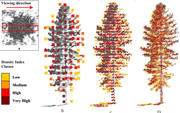
The method gave visually consistent results. Figure 3 compares the point cloud from the original scan and the values of the density index for Svoxels on a vertical slice of a black pine crown. The tree shape is well described by Svoxels with density index values apparently reasonable. However tree outline description quality is getting coarser when Svoxel size increases. Highest density values are logically located along the trunk and close to large branches. At a Svoxel density of 1m, the low density index values are located at the crown periphery. The tree back part is not as well described in the scan due to occlusion effects (shaded points). However no dissymmetry in density index can be noticed between the crown part facing the scanner system and the back part of the tree even though 3D laser point density largely differs between these two tree parts (Fig 3b, c, d). This confirms that the algorithm evaluates adequately the intercepted laser beams.
Figure 3: Density index were computed for the three grid dimension (0.25, 0.5, 1m). Density index are superimposed on their corresponding Svoxel centre on the lidar 3D point cloud. The results are given for a slice cut through a tree in the scan direction (a). Density index were separated into 4 classes using quartiles.
Viewing direction a Density Index Classes Low Medium High Very High Low Medium High Very High b c D
3.2 Comparative analysis of different tree crowns in a same scan
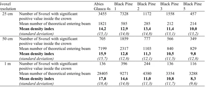
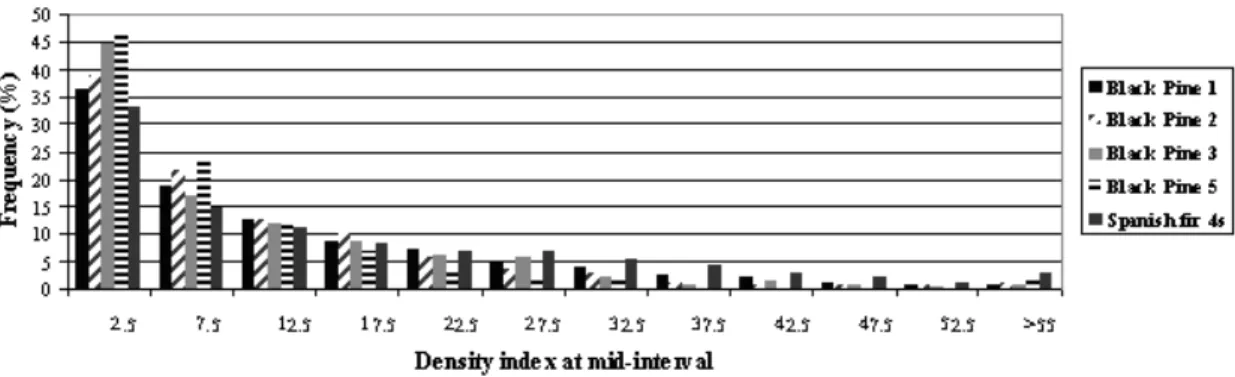
Results for the five selected trees are summarized in table 1. The number of Svoxels with a positive and significant density index decreases with the tree distance from the laser scanning system (related to the mean theoretical entering beam number). Similarly occlusion effects are more predominant with distance from the scanner depending on the obstacles in the path of the light beam. For example black pines 3 and 5 are located at a similar distance from the base station but occlusions are more numerous for black pine 5 located behind trees 1 and 2 (see figure 2). The mean density index is comparable for the five trees. But it tends to decrease with distance to the base station. Since only few trees were analyzed this could be due to natural tree heterogeneity. However, our initial results raise the possibility of a small bias. This bias could originate from partial occlusion of the incident beams. These effects, which increase with distance, are likely to increase the number of last returns with a weak intensity. These returns are not recorded by the system. The anomalies related to the distance can hence result from (1) an underestimation of lidar returns from the Svoxels and (2) a lower chance to record returns from trunks or large branches, which are characterized by high vegetation density but are partially occluded by crowns. Histograms of the density index values allow to compare the distribution for the 5 selected crowns for the three grid resolutions. Figure 4 presents the histogram for a voxel grid resolution of 50 cm. The histograms are comparable for all the pines. For the Spanish fir a slight difference can be noticed on figure 4 and was observed at all the 3 resolutions: density index frequencies are higher than those from the pines for densities ranging from 20 to 50. Consequently standard deviations were similar for all the black pine crowns and were higher for the Spanish fir (table 1). A higher foliage density for this species could explain this result. This open up the possibility to classify species using density index distribution.
Table 1: For each tree crown density index mean and standard deviation were computed for 3 grid resolutions: 25, 50 and 100 cm. The theoretical entering beam number gives an indication of the crown
distance from the lidar system.
Svoxel resolution Abies Glauca 4s Black Pine 1 Black Pine 2 Black Pine 3 Black Pine 5
Number of Svoxel with significant positive value inside the crown
3455 7328 1172 1558 457
Mean number of theoretical entering beam 1821 585 285 212 214 Mean density index 14,2 12,9 13,4 11,4 10,0 25 cm
(standard deviation) (15,1) (14,0) (14,8) (13,1) (13,2) Number of Svoxel with significant
positive value inside the crown
705 1859 777 566 349
Mean number of theoretical entering beam 7199 2317 1103 840 829 Mean density index 15,9 12,8 11,3 10,5 9,8 50 cm
(standard deviation) (15,7) (12,8) (12,1) (11,5) (12,8) Number of Svoxel with significant
positive value inside the crown
136 396 244 136 116
Mean number of theoretical entering beam 28405 9271 4380 3354 3288 Mean density index 17,8 14,6 11,0 10,8 8,3 1 m
(standard deviation) (18,4) (14,0) (11,3) (11,7) (9,6)
3.3 Comparison of density index for two scans
Table 2 recaps the results of the comparison of the 2 studied scans for two grid resolutions (0.5 and 1 m). The total number of Svoxels was calculated for a grid including the circular plot. After merging two scans from different locations we noticed that the no-data values represented only about 12 % of the total number of Svoxels in the plot for all grid resolutions. The voxel centers, for which a significant density index value was computed from both scans, are only about 55 % of the total number of Svoxels of the grid. This low value is explained by the fact that only the bottom part of the plot was scanned in the second scan. The significant differences in the
magnitude for the “Mean density index difference” and the “Mean difference for positive and significant density index values” are explained by a high number of Svoxels located in vegetation gaps. These Svoxels, with a null index value, are consistent between scans. Large differences in density index values are observed inside the vegetation elements. For the 50 cm grid resolution about 15 % of the density index values differ from less than 1 % and 45 % from less than 5% but 20 % of the Svoxels have index values with a difference higher than 20%. Part of these differences can be explained by (1) the difference between the Svoxel shapes observed from two points of view and (2) by the type of vegetation material hit by the laser beams. For example trunks or large branches can be sources of differences since they are not seen at the same place according to the base station location (back part of them, relative to view point, is occluded). Some differences may also be related to the potential bias we previously mentioned linking scan distance with density index value. All these hypotheses will have to be verified and possible bias need to be corrected before proposing a way to merge results from various scans. Lastly, we observed from the results that mean differences decrease with resolution while standard deviation increase. This tends to confirm the influence of large wooded elements present in the Svoxel on density index value differences. Actually, when grid resolution is getting coarser the proportion of large wooded elements inside the Svoxel decreases thus reducing the mean difference.
Figure 4: Histograms of density index values (positive and significant) for 5 tree crowns and for a Svoxel resolution of 50 cm.
Table 2: Results of comparison between density index values computed for two scans. Svoxel
resolution
Total number of Svoxel in
the grid
Mean difference of density indices (SD) [Number of Svoxels]
Mean difference for positive and significant density index values
(SD) [Number of Svoxels]
1 m 58499 -1,4 (6,4) [432175] -4,1 (11,5) [698]
50 cm 467999 -0,7 (5,4) [208531] -3,1 (16,1) [2266]
4. Conclusion
We proposed an innovative method to quantify spatial distribution in 3D of forest structure from terrestrial laser scanner data. The method rests on the hypothesis that the amount of laser beam returns inside a Svoxel (volume element defined in the lidar spherical coordinate system) is proportional to the density of vegetation material included inside this Svoxel. First results confirmed that our hypotheses are valid and that some adjustments can improve further the interrelationship between the lidar returns and the amount of forest components in the Svoxels. Visual and numerical analysis allowed verifying consistency of the derived density index values. However a slight bias could be noticed with a tendency of decrease in density index with distance from the base station position. This bias could originate from partial occlusions of the incident beams leading to a relative under sampling of trunks and large branches inside the 3D lidar point cloud when distance from the base station increases. Future work will focus on improving our algorithm, refining calculations, and correcting potential biases. In-depth analysis of scans
acquired in both first and last pulse modes and multi-scan comparisons at different grid resolutions also need to be tested out. Our analysis was an essential prerequisite for developing a method aiming at merging the different scans acquired on a same plot. This study was realized considering the prospect of establishing a link between airborne lidar data and field data with the aim of improving information extraction from airborne lidar data on forested areas. These results are very promising for the development of quantitative measures of the 3D forest structure that will meet the actual information needs in the fields related to forest ecology and management.
Acknowledgements:
This research was made possible though funding provided by the Centre National d'Etudes Spatiales (CNES). We are also thankful to the GIS Draix for its logistical support during the fieldwork.
References
Aschoff, T., Thies, M. and Spiecker, H., 2004. Describing forest stands using terrestrial
laser-scanning. In, XXth ISPRS Congress. International Archives of the Photogrammetry, Remote Sensing and Spatial Information Sciences, Istanbul, July 12-23, pp. 5.
Bienert, A., Scheller, S., Keane, E., Mohan, F. and Nugent, C., 2007. Tree detection and diameter estimations by analysis of forest terrestrial laser scanner point clouds. In: H.H. P. Rönnholm, J. Hyyppä (Editor). Proceedings of the ISPRS Workshop ‘Laser Scanning 2007 and SilviLaser 2007’. Espoo, September 12-14, 2007, Finland: 50-55.
Danson, F.M., Hetherington, D., Morsdorf, F., Koetz, B. and Allgöwer, B., 2007. Forest canopy gap fraction from terrestrial laser scanning. IEEE Geoscience and Remote Sensing Letters, 4(1), 157-160.
Fleck, S., Obertreiber, N.,Schmidt, I., Brauns, M., Jungkunst, H.F., and Leuschner, C., 2007. Terrestrial lidar measurements for analysing canopy structure in an old-growth forest. In: H.H. P. Rönnholm, J. Hyyppä (Editor). Proceedings of the ISPRS Workshop ‘Laser Scanning 2007 and SilviLaser 2007’. Espoo, September 12-14, Finland: 125-129. Hopkinson, C., Chasmer, L., Young-Pow, C. and Treitz, P., 2004. Assessing forest metrics with a
ground-based scanning lidar. Canadian Journal of Forest Research, 34(3), 573-583. Király, G. and Brolly, G., 2007. Tree height estimation methods for terrestrial laser scanning in a
forest reserve. In: H.H. P. Rönnholm, J. Hyyppä (Editor). Proceedings of the ISPRS Workshop ‘Laser Scanning 2007 and SilviLaser 2007’. Espoo, September 12-14, Finland: 211-215.
Lichti, D.D., Gordon, S.J. and Stewart, M.P., 2002. Ground-based laser scanners: operation, systems and applications. Geomatica, 56(1), 21-33.
Lim, K., Treitz, P., Wulder, M., St-Onge, B., and Flood, M., 2003. Lidar remote sensing of forest structure. Progress in Physical Geography, 27, 88-106.
Van der Zande, D., Hoet, W., Jonckheere, I., Van Aardt, J., and Coppin, P., 2006. Influence of measurement set-up of ground-based LiDAR for derivation of tree structure. Agricultural and orest meteorology, 141, 147-160.
Watt, P.J., and Donoghue, D.N.M., 2005. Measuring forest structure with terrestrial laser scanning. International Journal of Remote Sensing, 26(7), 1437-1446.
Wezyk , P., Koziol, K., Glista, M. and Pierzchalski, M., 2007. Terrestrial laser scanning versus traditional forest inventory. First results from the Polish forests. In: H.H. P. Rönnholm, J. Hyyppä (Editor). Proceedings of the ISPRS Workshop ‘Laser Scanning 2007 and SilviLaser 2007’. Espoo, September 12-14, Finland: 424-429.