Agile flight control techniques for a fixed-wing aircraft

Agile Flight Control Techniques for a Fixed-Wing

Aircraft

by

ARCHIVES

Frantisek Michal Sobolic

B.S., Aerospace Engineering

University of Michigan (2006)

Submitted to the Department of Aeronautics and Astronautics

in partial fulfillment of the requirements for the degree of

Master of Science in Aeronautics and Astronautics

at the

MASSACHUSETTS INSTITUTE OF TECHNOLOGY

June 2009

@

Massachusetts Institute of Technology 2009. All rights reserved.

Author...

...

Depa ment of Aeronautics and Astronautics

/"

_May

Certified by...

Jonathan P. How

Professor

Thesis Supervisor

Accepted by...

Prof. DaiL . barmofal

Associate Department Head

Chair, Committee on Graduate Students

MASSACHUSETTS INSTITUTLE

OF TECHNOLOGY

JUN 2 4 2009

LIBRARIES

Agile Flight Control Techniques for a Fixed-Wing Aircraft

by

Frantisek Michal Sobolic

Submitted to the Department of Aeronautics and Astronautics on May 22, 2009, in partial fulfillment of the

requirements for the degree of

Master of Science in Aeronautics and Astronautics

Abstract

As unmanned aerial vehicles (UAVs) become more involved in challenging mission objectives, the need for agility controlled flight becomes more of a necessity. The ability to navigate through constrained environments as well as quickly maneuver to each mission target is essential. Currently, individual vehicles are developed with a particular mission objective, whether it be persistent surveillance or fly-by reconnais-sance. Fixed-wing vehicles with a high thrust-to-weight ratio are capable of perform-ing maneuvers such as take-off or perch style landperform-ing and switch between hover and conventional flight modes. Agile flight controllers enable a single vehicle to achieve multiple mission objectives. By utilizing the knowledge of the flight dynamics through all flight regimes, nonlinear controllers can be developed that control the aircraft in a single design.

This thesis develops a full six-degree-of-freedom model for a fixed-wing propeller-driven aircraft along with methods of control through nonconventional flight regimes. In particular, these controllers focus on transitioning into and out of hover to level flight modes. This maneuver poses hardships for conventional linear control archi-tectures because these flights involve regions of the post-stall regime, which is highly nonlinear due to separation of flow over the lifting surfaces. Using Lyapunov back-stepping control stability theory as well as quaternion-based control methods, control strategies are developed that stabilize the aircraft through these flight regimes with-out the need to switch control schemes. The effectiveness of each control strategy is demonstrated in both simulation and flight experiments.

Thesis Supervisor: Jonathan P. How Title: Professor

Acknowledgments

First, I would like to thank Raytheon Missile Systems for their support during my graduate school experience in which I am able to advance both my education and my

career.

Secondly, I would like to thank Professor How for his guidance and wisdom during my research pursuits at MIT. His constant curiosity with the challenges that I faced and his helpful notions gave me the direction to successfully complete my research.

The members of the Aerospace Controls Laboratory have been extremely support-ive throughout my work on this thesis. I would like to offer a special thanks to Buddy Michini, who offered continual guidance throughout my work, especially with soft-ware and hardsoft-ware issues. I would also like to thank Cameron Fraser, Josh Redding, Karl Kulling, Sergio Cafarelli, Frank Fan, Samera Ponda, Dan Levine, Brett Bethke, Brandon Luders, Andrew Whitten and Kenneth Lee for the specific ways in which they have assisted me. I would also like to thank Kathryn Fischer for her support and resourcefulness throughout my time here.

During the dynamic modeling phase of my project, I received invaluable technical support from Dave Robertson, Richard Perdichizzi and Todd Billings. I would like to thank them for guidance and technical advice.

Finally, my family and friends have been a constant source of love, support and inspiration for me throughout my education. My parents, Frank and Maryanne have always been there in many ways to support my aspirations as well as my Aunt Diane and Uncle Tom who supported me and have always been interested in my educational pursuits.

Contents

1 Introduction

1.1 M otivation ... 1.2 Background ...

1.2.1 Quaternion . ...

1.2.2 Lyapunov Backstepping Design . . 1.3 Literature Review ... 1.4 Contributions ... 1.5 Approach . ... 2 Modeling 2.1 Introduction ... 2.2 Preliminaries . ... 2.2.1 Nomenclature . . . . 2.2.2 Vehicle Description . . . . 2.2.3 RAVEN Testbed . . . .. 2.3 Tests Performed ... 2.3.1 Introduction ... 2.3.2 Prop-Hang Test ...

2.3.3 Quasi-Steady State Wind Tunnel Test 2.4 Equations of Motion ...

2.4.1 System Identification ...

3 Quaternion Based Control 3.1 Introduction ...

3.1.1 Notation . . . . 3.2 Inner Attitude Loop . . . . 3.3 Outer Velocity Loop . . . . 3.4 Thrust Controller . . . . 41 41 42 42 44 46 I :

3.5 Results ... 3.5.1

3.5.2 3.5.3

Simulation ...

Decoupled Roll Control. Transition to Level-Flight

4 Nonlinear Lyapunov Backstepping Controller

4.1 Introduction . . . . 4.2 Controller Outline . . . . 4.2.1 Simulation . . . . 4.3 Linearized Hover Controller . . . 4.3.1 Flight Test . . . . 4.4 Lyapunov Quaternion Control . . 4.4.1 Introduction . . . . 4.4.2 Simulation . . . . 4.4.3 Hardware Implementation

5 Conclusion

5.1 Future Work ...

5.1.1 Improved Dynamic Model . 5.1.2 Trajectory Linearized Control 5.1.3 Path Feasibility Planner .

A Quaternion Based Method for the Determination using a Motion Capture System

A. 1 Introduction ...

A.2 Extracting the Axis Angle ...

of Body Rates 85 85 86 53 53 54 59 61 65 67 67 70 72

List of Figures

1-1 General Atomics Aeronautical Systems Predator B . ... 14

1-2 AeroVironment Raven B UAV ... 14

1-3 Bell Boeing V-22 Osprey ... 15

1-4 Lockheed Martin X-35B Joint Strike Fighter . ... 15

2-1 Vehicle and hardware used for controller implementation ... . 23

2-2 Modeling test setup and load cell placement . ... 25

2-3 Aircraft mounted with tinsel hung around control surfaces to determine propeller downwash diameter ... ... 27

2-4 Linear least square fit of the radius of the cone produced by propeller downwash .. ... . .. .. . .. .. ... ... ... . . ... 27

2-5 Estimated and actual propeller downwash flow located at the respective control surfaces .. ... ... .. .. .. . ... .. ... . . ... .. 28

2-6 Moment coefficient as a function of respective control surface deflection angle . . . .. .. . 29

2-7 Wind tunnel test setup -mounted upside down due to maneuverability constraints . . . .. . 29

2-8 Sample wind tunnel moment data taken at 300 angle-of-attack . . .. 30

2-9 Effect of propeller downwash combined with the free-stream velocity . 31 2-10 Aircraft body and inertial coordinate frames . ... 31

2-11 Measured versus theoretical force coefficients for various free-stream velocities . . . .. . 34

2-12 System Identification: compared state outputs for the sinusoidal ve-locity test . . . .. .. . 37

2-13 Stills from the Clik transition maneuver . ... 39

2-14 System Identification: compared state outputs for the hover to transi-tion test . . . .. .. . 40

3-2 Vector description of additional body x-velocity necessary to obtain desired inertial velocity .... .... .... ... ... .. 46 3-3 Roll decoupling maneuver state output . . . . .. . . . . 50 3-4 3-D visualization of the quaternion controlled transition maneuver . . 51 3-5 Position output for the quaternion-based control transition maneuver 51 3-6 Various state results for the quaternion-based controlled transition to

level-flight . . . .. . . . . . 52 4-1 _{Lyapunov-based backstepping control architecture . . . . . 53} 4-2 Simulated Lyapunov-based backstepping control in hover with initial

condition offsets ... ... ... .. 60 4-3 Lyapunov-based backstepping take-off to hover simulation ... . . 61 4-4 Experimental linearized Lyapunov-based controller position data about

hover ... ... ... 66

4-5 Lyapunov quaternion control architecture . ... ... . 68 4-6 Sample transition trajectory data with radial basis least square fit . . 70 4-7 Simulated Lyapunov quaternion controlled hover to hover state data . 73 4-8 Simulated Lyapunov quaternion controlled hover to hover control effort 74 4-9 Hardware implemented Lyapunov quaternion controlled hover to hover

state data . . . ... . . . .. . 75 4-10 Hardware Lyapunov quaternion controlled hover to hover control effort 76 4-11 Measured y-position output for the hover to hover maneuver varying

the feed-forward predictive gains .. ... ... 76 4-12 Elevator deflection output for the hover to hover maneuver varying the

model feed-forward gains ... 76

4-13 Hardware implemented Lyapunov quaternion controlled take-off to hover m aneuver . . . .. . . . ... . .. . 77 4-14 Lyapunov quaternion controlled take-off to hover state data ... . . 78

4-15 Lyapunov quaternion controlled take-off to hover control effort . . . . 79

5-1 Trajectory linearized control architecture .. . ... 83

A-i Quaternion data due to a pure rotation about the reference z-axis... 87

A-2 Pure body z-rotation illustrating axis flip . . . ... . .... . . . . .. 88 A-3 Continuous quaternion data due to a pure rotation about the reference

List of Tables

Clik aircraft parameters . . . . Clik aerodynamic parameters . . . . Simulation quaternion attitude loop gains . . . Algorithm to convert from DCM to quaternion . Radial basis function values: a = 1.2 . . . .

Smooth quaternion signal data algorithm . . . .

2.1 2.2 3.1 4.1 4.2 A.1 S . . . . .. . . . . . . . . . . . . . . . . . . . . . ...

Chapter 1

Introduction

Unmanned aerial vehicles (UAVs) are becoming increasingly involved in challenging mission objectives including search and rescue, reconnaissance and other intelligence-gathering roles. The advantage of these vehicles is not only the absence of human presence in a volatile scenario, but also their production value relative to manned vehicles. In general, two types of UAVs are produced, remote piloted and self-piloted. Remote piloted UAVs allow an operator to control the vehicle to perform a mission objective while a self-piloted UAV performs a mission autonomously based on a set of rules preprogrammed prior to flight. Autonomous UAVs are much more complex system, however, emerging technologies would allow them to address much more complex missions.

Even under the categroy of technologically advanced aircraft, classes of UAVs are built to perform tasks based on specific mission scenarios. For instance, the General Atomics Aeronautical Systems Predator, shown in Figure 1-1, is a very common and very well known UAV designed for long-endurance, medium altitude remotely con-trolled surveillance and reconnaissance operations. With a wingspan of 66ft, weight of 10,0001bs and operational duration of more than 40 hours, this aircraft is able to provide both a front line soldier and operational commander real-time footage with its on-board vision system [1]. The AeroVironment Raven (Figure 1-2), also used for surveillance and reconnaissance but at low altitude, is a highly mobile, light weight aircraft that can be operated manually or programmed for autonomous operation [2].

Figure 1-1: General Atomics Aero- Figure 1-2: AeroVironment Raven nautical Systems Predator B B UAV

Each of these UAV classifications have an important role in their aerial missions. For a particular mission, multiple UAVs may be used to provide feedback on related issues from different perspectives. With these various specified aircraft systems, clas-sifications have been made to separate vehicles by the roles which they fulfill yet vehicles that are able to perform multiple missions could declare UAV dominance. An individual UAV is only limited by the user, the amount of autonomy it is granted and the overall capabilities of the aircraft. By advancing the capabilities, thus ex-panding the range of mission qualifications, a single UAV may be used for multiple mission scenarios.

1.1

Motivation

An aircraft with short take-off and landing (STOL) and vertical take-off and landing (VTOL) capabilities has been an active area of research for many reasons. One of the main interests is their ability to maneuver and land in a constrained environment

and still have the fuel efficiency and quickness to proceed to another location. One such vehicle is the Bell Boeing V-22 Osprey shown in Figure 1-3. It is a tiltrotor aircraft with the combined STOL and VTOL capabilities. The vehicle can take-off and land similar to a helicopter and hover at a single position above ground. Once airborne, its engine nacelles can be rotated to convert the aircraft to a turboprop airplane, capable of high-speed, high-altitude flight [3]. There are many reasons

Figure 1-3: Bell Boeing V-22 Os- Figure 1-4: Lockheed Martin

X-prey 35B Joint Strike Fighter

why this aircraft seems so attractive for multiple missions. Its capabilities include: transporting troops and cargo, air-to-air refueling and landing aboard an aircraft carrier compacting its storage area by retracting its rotors. Another type of vehicle is the X-35B Joint Strike Fighter produced by Lockheed Martin shown in Figure 1-4. This vehicle also has combined ability features that allow it to proceed in a short take-off and vertical landing (STOVL) manner. The nozzle, which is supplemented by two roll control ducts on the inboard section of the wing, together with the vertical lift fan provide the military required STOVL capability [1]. These combined capabilities allows the aircraft to carry a larger payload during take-off and land in constrained environments. Versatile aircraft such as these are in high demand, and it seems therefore fitting to develop UAVs with similar capabilities. UAVs have the potential to maneuver much more aggressively due to the lack of a human pilot, yet controlling them through such maneuvers remains a challenge, even today.

The UAVs that have been designed thus far are built for a mission specific scenario. For a reconnaissance mission, fixed wing vehicles are constrained to fly at speeds above stall limiting them to perform a loitering pattern for persistent surveillance. On the other hand, vehicles such as quadrotors and helicopters have a hovering ability but are hindered by their efficiency in translating from one mission location to the next. However, a vehicle designed to capture the strengths of both a fixed and rotary wing aircraft could be used in either situations and provide this sought-after versatility.

The objective of this thesis is to design a agile flight controller for a fixed wing aircraft, enabling it to follow a desired trajectory through multiple regimes of flight,

including post-stall. Such a controller will enable the aircraft to hover as well as safely transition to steady-level flight. It will also inhabit the capabilities of conventional take-off and landing as well as a perch style landing. With these combined abilities, the agile flight controller gives an aircraft the desirable characteristics of the versatile, manned vehicles mentioned previously.

1.2

Background

1.2.1

Quaternion

A quaternion is a 4-dimensional vector used to describe the transformation of a vehicle

in 3-dimensions. The use of quaternions are sometimes favored over other descriptors due to their non-singularity properties at any aircraft attitude. Traditional aeronautic transformations (Euler angles), are hindered by a phenomenon known as gimbal lock. Gimbal lock causes a loss of degree of freedom (DOF) which could lead to controller instability. Since this thesis explores aggressive flight regimes, a quaternion attitude descriptor was chosen to provide a singularity-free rotation from hover to horizontal flight.

1.2.2

Lyapunov Backstepping Design

Lyapunov backstepping control provides a stable controller by developing a promi-nent functional candidate that satisfies the Lyapunov criteria, known as the control

Lyapunov function. The backstepping technique can be summarized as follows:

1. Start with the state furthest from influential control actuators.

2. Introduce a virtual state and a control. 3. Define a control Lyapunov function.

4. Choose the virtual controller such that the control Lyapunov function satisfies the Lyapunov criteria.

5. If the virtual controller involves a control actuator, this is the control law, if not repeat Step 2 with the new virtual state.

These control Lyapunov functions "step" through the dynamics of a system leading to a control methodology that can be used to produce a desired response.

1.3

Literature Review

This research is focused on the aggressive maneuvering of UAVs in a constrained environment. Aggressive maneuvers at low speed require a special type of vehicle capable of maintaining stability and a high level of performance during unconventional missions. This section gives a historical perspective of the previous work done in the areas of aggressive and agile flight and is coupled with a discussion of the control techniques used.

A number of researchers have recently investigated the idea of developing fixed-wing aircraft with hovering capabilities. The first successful manually controlled tran-sitions were performed in 1954 with the Convair XFY-1 "Pogo" [4]. Additionally, a custom designed, radio-controlled (R/C) airplane was developed at Drexel Univer-sity [5], and possessed the capability to fly in both level-fight and hover. The airplane was manually controlled in level-fight operations and transitioned to a computer-controlled hover configuration upon user input. Successful autonomous transitions from steady level-flight to hover (and vice-versa) have also been performed by re-searchers at Georgia Tech on a R/C airplane [6]. Rere-searchers from the Massachusetts Institute of Technology successfully demonstrated an autonomous fixed-wing aircraft with the capability to take-off, hover, transition to and from level-flight, and perch on a vertical landing platform. These maneuvers are all demonstrated in the highly space-constrained environment of the Real-time indoor Autonomous Vehicle test En-vironment (RAVEN) at MIT [7]. The developed flight control system in [7] has two linear controllers designed independently for hover and level-flight configuration. Intelligent switching between these two controllers enables the aircraft to perform transitions from level-flight to hover, and visa-versa.

The control techniques mentioned above are limited to performing in a region pre-scribed by the linearization method used. Full knowledge of the aircraft's dynamics, including nonlinearities, could solve potential issues of needing multiple controllers in different flight modes and a single control design could be realized. The use of nonlinear controllers provide means of control at all possible flight regimes so, non-linear decoupling theory and dynamic inversion approaches have been applied to flight control systems [8], [9]. Unfortunately, it was shown that an inverse dynamic approach, even when the dynamics are very well known, may result in the desired lin-ear input/output response but may also include undesirable unstable zero dynamics. Nonlinear Lyapunov-based controllers have the ability to overcome some of these is-sues [10-13]. In particular, the backstepping approach is used when a vehicles states are influenced through other states. This technique is demonstrated in [14] for a 6-DOF mid-altitude unmanned airship, where a simulated airship tracks a desired trajectory. They prove that the tracking error will converge exponentially to zero since the proposed controller is globally asymptotically stable. Also, [13] demon-strates the same type of trajectory-tracking capability in simulation for a hovercraft moving on a planar surface and an underwater vehicle moving in 3-D space. It is important to note that this control law assumes no parametric uncertainty, there-fore an onboard estimator is implemented to predict the values of the states used for feedback in the Lyapunov control algorithm.

The work presented in this thesis follows the work of [13] and [15] to control an aircraft from hover to translational flight. In [15], Knoebel uses an adaptive quaternion-based attitude controller to maintain aircraft performance through poorly known regions of the vehicle dynamics during a transition from hover to level-flight. Gain scheduling was used based on the sensed airspeed over the control surfaces. On the other hand, [13] forms a Lyapunov backstepping controller such that all the closed-loop signals are bounded and the tracking error converges to a neighborhood of the origin that can be made arbitrarily small. It has the capability of following a prescribed trajectory solely based on the vehicles dynamics. Therefore, an accurate and complete model of the system dynamics must be known through all regions of

movement.

1.4

Contributions

Each of the following chapters provide a unique contribution to the overall goal of a transition controller, which are summarized below.

* Chapter 2: A full nonlinear dynamic model is derived for a specific vehicle which serves as a testbed for all controllers through simulation and hardware implementation. The process of achieving this high-fidelity model is presented through extensive wind-tunnel and static experimentation. A full system iden-tification is performed to verify the input/output response through the use of an off-board motion capture system which provides the necessary vehicle state information.

* Chapter 3: A quaternion-based attitude controller is presented following the

work of Ref. [15], but is modified for reference velocity tracking. The velocity error is used to provide the quaternion controller with the desired attitude in order to decrease the velocity error. Controller results are presented in simula-tion as well as hardware implementasimula-tion. A full transisimula-tion from hover to level flight and back to hover is shown.

* Chapter 4: A general Lyapunov backstepping technique is introduced with trajectory tracking capabilities. This technique is then applied in simulation to the derived dynamics and the results are shown. To implement this design on hardware, a modified version of Ref. [13] is used that combines the rotational rate tracking capabilities of the quaternion attitude controller, with the state to state influential approach of the backstepping design. Both simulation and hardware results are shown for various trajectories.

1.5

Approach

This thesis is structured as follows. Chapter 2 introduces the fixed-wing aircraft which serves as the vehicle testbed for all of the controllers developed. Here the equations of motion are derived and a full system identification is performed. In Chapter 3, a quaternion-based attitude controller with the ability to follow user defined velocity commands is derived. Chapter 4 introduces a Lyapunov backstepping controller with the ability to follow a user defined position trajectory modified with the quaternion controller and implemented in hardware. Finally, Chapter 5 provides concluding remarks as well as suggested future work.

Chapter 2

Modeling

2.1

Introduction

In order to control a system effectively, a good understanding of the dynamics and its effects on the environment must be modeled. The more that is known about the system, the more affective the controller can be. Controllers developed about linearized models are often used but limit the vehicles ability to the neighborhood encompassing this linear region. One of the most challenging parts in designing a control system for most vehicles is the complexities and interrelated dynamics present, thus a lot of time and effort is contributed to the modeling process.

For fixed-wing aircraft, the dynamics associated with pre-stall configurations are well known and have been studied since early flight. However, performing agile aggressive flight requires an aircraft go beyond the pre-stall configuration and into the poorly understood post-stall flight regime. In the following chapter, a detailed description of the tests that were performed in order to obtain these equations of mo-tion (EOM) is given. Multiple tests are compared to theoretical findings, in particular predictions made using flat plate theory which describes the entire flight regime par-ticularly well at low Reynolds numbers (< 104). Finally, the EOM are compared to actual flight test data recorded in the Real-time indoor Autonomous Vehicle test EN-vironment (RAVEN) concluding that the system identification validates the models

2.2

Preliminaries

In the following sections the experimental aircraft as well as the notation and nomen-clature are introduced. This aircraft is used throughout the rest of the controller implementation in this thesis. Due to the complexities of modeling, standard aero-dynamic notations presented in [16] and [17] are used.

2.2.1

Nomenclature

p = Vehicle position vector, m v = Velocity vector, m/s

w = Angular rate vector, radians/sec

q = 4-Dimensional unit quaternion

R, = Rotation matrix from vehicle body to inertial frame

uW = Control surface deflection input vector, radians

m = Mass of the aircraft, kg

a = Angle-of-attack of the wing, radians

p = Density of air, kg/m3

6t = Thrust, N

(')d = Desired value

()e = Error value

()a = Measured value

( = Details pertaining to the propeller )w = Area affected by propeller downwash

()nw = Area not affected by propeller downwash

(')ref = Reference

()I = Inertial frame

2.2.2

Vehicle Description

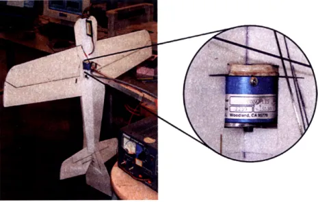
To facilitate the implementation of various controllers, a slightly modified version of the high performance Clik [18] indoor aerobatic plane designed by RC Factory is being used, shown in Figure 2-1(a). This aircraft is extremely maneuverable due to its large control surfaces and high thrust-to-weight ratio. The vehicle is equipped with an Axi Brushless Out-Runner 2203/52 motor with a 20cm Grapner Slowfly Propeller which provides a thrust-to-weight ratio in excess of 1.4. Control deflection actuation is provided by three GWS pico standard servo motors and receives commands on a GWS four-channel micro receiver. The aircraft is also equipped with a 400mAh 2-cell lithium polymer battery which delivers power to an 8-amp JETI electronic speed controller shown in Figure 2-1(b).

(a) Indoor aerobatic Clik air- (b) Vehicle hardware components craft

Figure 2-1: Vehicle and hardware used for controller implementation

The vehicle is extremely light for its size, weighing approximately 170 grams due to the use of 2.8mm thick Dapron foam material for its body and carbon fiber strips to reinforce structurally weak areas. The aircraft is symmetric about body x-z axes (see Figure 2-10) and made up of flat plates. The total length of the vehicle is 90cm with a wingspan of 84cm and the inertial as well as the surface area estimation is provided through the use of SolidWorks CAD modeling software. More vehicle parameters and details are given in Table 2.1.

Table 2.1: Clik aircraft parameters

Parameter Description Value Units

A? Aspect Ratio 4.2

d _{Propeller diameter 20.0 cm}

Aap Area of aileron induced by propeller downwash 0.00150 m2

Ae Area of the elevator 0.03226 m2

Ar Area of the rudder 0.03123 m2

Aanw _{Area of the aileron in the free-stream} 0.024 m2

IXX x-Moment of Inertia 0.00143 kg- m2

I y-Moment of Inertia 0.00610 kg- m2

Izz z-Moment of Inertia 0.00737 kg. m2

Lap Moment arm of the aileron 0.080 m

affected by prop-wash

Lep Moment arm of the elevator 0.533 m

(cg to center of pressure)

Lrp Moment arm of the rudder 0.631 m

(cg to center of pressure)

Lanw Moment arm of the aileron 0.23 m

free-stream induced

2.2.3

RAVEN Testbed

Vehicle position and attitude sensing is done off-board through the Real-time indoor Autonomous Vehicle test ENvironment (RAVEN), eliminating the need for onboard sensors which typically are expensive and add unwanted weight. RAVEN provides a well equipped, robust platform for the rapid prototyping of controllers applicable to many different vehicles. This testing environment uses a position and orientation tracking system with an update rate of 120 Hz, minimal delay (20-30msec) and sub-millimeter accuracy with the use of Vicon motion capture camera system [19]. A single camera can be seen at the top of Figure 2-1(a) as the black object with the red ring. The only requirement is that the vehicle be equipped with reflective dots which the cameras use for object recognition.

Since only position and attitude data are directly measured by the system, the states time rate of change must be taken to acquire rate data. This is done by the process of a Kalman filter to attenuate noise produced by differentiating. The filter requires that smooth continuous data is used as the input. Quaternion data however,

is not a smooth continuous signal by the process of extraction, so a special algorithm is implemented to ensure smoothness which is outlined in Appendix A. From this tracking system, state data such as position, velocity, attitude and rotational rate is computed and used for full-state feedback. The state data is then routed to a computer which processes the desired control commands. These control commands are then sent to the R/C transmitter which relays the respective commands to the vehicle, closing the control loop.

2.3

Tests Performed

2.3.1

Introduction

To accurately identify the dynamic model, a JR3 6-axis load cell is placed at the center of gravity which allowed steady-state force and moment data to be taken for all 3 axes (load cell configuration shown in Figure 2-2). With the aid of a low pass filter

Figure 2-2: Modeling test setup and load cell placement

to attenuate high frequency noise, the multi-axis load cell is able to measure forces within 10-3 Newtons and moments within 10-2 Newton meters. Two main types of tests were performed, prop-hang and wind tunnel tests. A prop-hang is when the force used to balance out the vehicles weight is solely provided by the propeller thrust.

These tests were performed with the intent of determining the specifics of the vehicles dynamics at high angles-of-attack during a hover to level-flight transition.

2.3.2

Prop-Hang Test

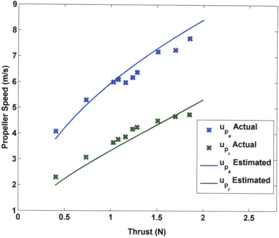
The prop-hang was the first test done and was primarily used to determine the specifics of individual axis moment data and propeller downwash velocity. The pro-peller downwash velocity is defined as the induced velocity created by the spinning blade and is found by using aspects of propeller momentum theory and conservation of mass as in [7] and [20] and based on inviscid, incompressible flow assumptions. A similar approach is used here but modified experimentally under the assumption that the flow created is in a uniform conical form as a function of the thrust command and distance from the propeller blades instead of a stream tube that extends infinitely and uniformly far downstream. This is an approximation for attempting to capture the loss of efficiency due to the slipstream rotation of the fluid within and outwards from the stream tube, which is one of the major objectives propeller momentum theory. The approximation assumes that the conical formation, in the limit, will approach a pure cylindrical shape as the thrust is increased. In order to measure the radius of the assumed cone shape as a function of distance and thrust, pieces of tinsel were pieced along both the aileron and rudder/elevator control surfaces as shown in Fig-ure 2-3. The thrust is varied to determine the granularity spacing of the tinsel which is necessary to produce an accurate measurement. Figure 2-4 shows a linear least squares fit to the measured radius as a function of thrust. With the cross-sectional area estimated, the flow created is approximated by [20]

u,(t, 1)= U _ U (2.1)

4 2pAdisk (t, 1) 2

where u, is the magnitude of the free-stream velocity given as

x Aileron Xx _{x Rudder} 0.22 X X x ::: XXX So0.2 _X 0.18 0 .164 0.12- X X X X X X X X X X X X X X X X X 0.1 0 0.5 1 1.5 2 2.5 Thrust (N)

Figure 2-3: Aircraft mounted with tin- Figure 2-4: Linear least square fit of the sel hung around control surfaces to de- radius of the cone produced by propeller termine propeller downwash diameter downwash

Assuming that during a prop-hang their is no free-stream velocity present, Equa-tion 2.1 reduces to

Up(t, 1)= 2pAd (t, (2.3)

2pAdisk Ot 1)

where Adisk(6t, 1) is determined experimentally and represents the cross-section of the conical region as a function of thrust (6t) and distance (1) from the propeller. The

propeller downwash velocity is presented as Upa or Up,, depending on whether the

aileron (a) or rudder/elevator (r) is the particular aerodynamic region of interest. The rudder and elevator calculations are done together due to very similar measure-ments and distance from the propeller. Actual measuremeasure-ments were taken using an

anemometer and comparisons are shown in Figure 2-5.

The prop-hang test provides means to estimate the moment coefficients for the control surfaces by using the combination of thin airfoil theory and Prandtl's lift-line theory [17] by

1

M = Ppu ,Cj/Ae/rLe/r. (2.4)

the-8 76 -0' 5 u Actual -u Estimated 2P 0 0.5 1 1.5 2 2.5 Thrust (N)

Figure 2-5: Estimated and actual propeller downwash flow located at the respective control surfaces

ory predicts that for an infinite flat plate, C, is approximated by a value of 27r. A correction accounting for a finite aspect ratio for each surface must be taken into account [21] by

CL- 1 + (2.5)

With the load cell placed at the center of gravity of the vehicle and thrust approx-imately equal to the weight, measurements were taken to determine the moment created with each control surface deflection. Figure 2-6 shows a comparison between the theoretical and measured moment data about an individual aircraft body axis. Aileron control authority is limited during a prop-hang due to the lack of down-wash over these control surfaces. Measurements taken were primarily in the noise of this particular instrument and could not be physically determined. An estimate

XXX x 0.201 0.10--0.00 -0.10 4.20--0.25 0.156 0.10 0.0os -0.00 40.2 /xxx

Figure 2-6: Moment coefficient as a function of respective control surface deflection angle

Figure 2-7: Wind tunnel test setup - mounted upside down due to maneuverability constraints

of the propeller drag and moment contribution of the ailerons are discussed more in Section 2.4.

2.3.3

Quasi-Steady State Wind Tunnel Test

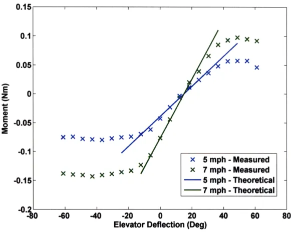
The vehicle was tested at multiple free-stream conditions in the wind tunnel (see Figure 2-7). The first set of tests were done at 5 degree increments of angle-of-attack without the propeller on to obtain nominal aerodynamic coefficients. The primary ob-jective was to gain insight on the moments produced by the body/elevator deflection combination. Since elevator coefficient data has been determined in Section 2.3.2, the

x x x x Measured

- Thin Airfoil Thory

-40 -20 0 20 40 60

Elevator Deflection (Degrees)

(a) Elevator moment coefficient

02% .

xxx x/ x Measured

x - Thin Airfoil Theory

40 40 -20 0 20 40 60

Rudder Deflection (Degrees)

0.151 1 1 I 1 Ir x x x x XXXX _X x xx x 5 mph -Measured x x x xxx x X x 7mph Measured - 5 mph - Theoretical -7 mph -Theoretical -60 -40 -20 0 20 Elevator Deflection (Deg)

Figure 2-8: Sample wind tunnel moment data taken at 300 angle-of-attack

aircraft moment due to angle-of-attack (Cm,) is found by

CmO 0 m - Cm6e 6e _(2.6)

Examples of the data found can be seen in Figure 2-8.

Next, tests were performed while incrementing the elevator and throttle com-mands. It was determined that the vehicle aerodynamic dynamics over the wing be split into two parts, the area in which the propeller downwash affects the aircraft, de-noted by (.)w, and the free-stream-only non-affected areas, (-)nw. The area affected by the propeller downwash also experiences the free-stream velocity shown in Figure 2-9. The resulting airspeed and angle-of-attack are given by

0.1 0.05s -0.05 -0.1--0.15 40 60

Figure 2-9: Effect of propeller downwash combined with the free-stream velocity

UWa/, u u2a/r P= + 2uup, cos(a) (2.

aw/r = arctan -+

VX + up./,

7)

(2.8)

The rest of the wind tunnel aerodynamic data is presented in the next section.

2.4

Equations of Motion

xB

B

<

zBI

Figure 2-10: Aircraft body and inertial coordinate frames

The set of nonlinear differential equations follows the baseline model described in [16] using Newton's second law for rigid-body dynamics but modified for this particular aircraft's kinematics and dynamics. Equations are in the aircraft body

frame (shown in Figure 2-10) given by

= RIBB, (2.9)

R4 = RS(W B), (2.10)

JB = -S(wB)JwB + fw + Gwuw, (2.11)

MyB = -S(wB)MvB + fv + gv6_{t. (2.12)}

where the mass, inertia and thrust force directional matrices are respectively,

m 0 0 IX 0 0 1

M= 0 m 0 , J= 0 , gV 0

0 0 m 0 0 Izz 0

Due to the symmetrical build of the aircraft, the cross-coupled inertia tensor terms

Ixy, Ixz and Ivz are considerably smaller than the coupled terms and are disregarded.

The angular velocity cross-product matrix, moment decoupling matrix and control surface deflections are

0 -Wz y g9 0 0 6a

S(w) = wz 0 -w , G 0 922 0 uW 6e

-- Wy W 0 0 0 933 6r

where

911

922 PUwrC Le AeLep (2.13)

1 2 W CL , L

g33 "PUwr CLT Ar Lr

The constant parameters (Aanw, Aap, A, A,) and (Lanw, Lap, Lep, Lrp) are the

respec-tive aileron, elevator and rudder areas and moment arms given in Table 2.1. In Equation 2.13, the difference in the form of g11 is due to the fact that only part of the wing area is affected by the propeller downwash while the rudder and elevator control surfaces are always engulfed. Although the propeller downwash conical area

changes as a function of thrust and distance, it deviates very little over the wings and is modeled as a constant (see Figure 2-4). Development of the remaining force and moment terms will be based on this assumption. This assumption is a major contrib-utor to the total force and moments created because of the low Reynolds number in which the aircraft is flying through, 104.

The force vector f, is the sum of the gravitational and aerodynamic forces in the body frame, given in Equation 2.14.

0

- cos(a) 0

sin(a)

Drag

1

fv

-mg -sin(a) 0 cos(a) Lift CD_ Vz

The first term involves the transformation of weight from the inertial to body frame. The second term comprises the aerodynamic contribution of lift and drag forces. Since these are in the wind frame a rotation matrix pre-multiplies the aerodynamic terms to obtain the desired forces in the body frame. The last term in Equation 2.14 represents the viscous drag that is induced by translating through the air. Drag and lift forces are divided into two sections and are described as

1 2 C D + U2 C nw )

Drag = p

(

Lift = 2wCLwSw LSnw) (2.16)

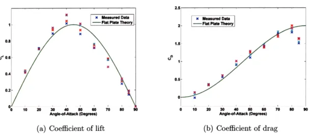
Figure 2-11 shows the coefficients of lift (CL) and drag (CD) for the free-stream section. Since this aircrafts main lifting surface is without camber, the coefficient of lift is symmetric about the body x-y axes. Note that the measured data is in agreement with flat plate theory [22], where

CL = 2 sin(a) cos(a) CDo = 2 sin2_{(a). (2.17)}

The areas affected by the prop-wash experience an angle-of-attack < 20 degrees (de-termined by measuring flows then using Equation 2.8) due to the contribution of

10 20 30 40 so go Angb-of-Atack(Degroe)

(a) Coefficient of lift

Figure 2-11: Measured versus velocities

30 40 k (D A 0 70 Angle-of4Atack (Degres) (b) Coefficient of drag

theoretical force coefficients for various free-stream

the additive propeller flow, and thus Prandtl's classical lifting-line theory [17] can be used:

CLw --- C Law awa

C2D CDW = ow + _reAT?

These also need to be corrected for a finite wing by Equation 2.5. Descriptions of the various parameters are given in Table 2.2. The term f, in Eq. 2.11 represents the

Table 2.2: Clik aerodynamic parameters

Parameter Description

e Oswald efficiency factor

CL6, Aileron coefficient of lift

CL6e Elevator coefficient of lift

CL , Rudder coefficient of lift

CDw, Effective drag coefficient

CLawa Effective lift coefficient

Cm,w Moment coefficient from effected propeller downwash

Cmanw Moment coefficient from free-stream velocity

c Moment arm from effected propeller downwash

lnw Moment arm from free-stream velocity Sw Wing area effected by propeller downwash

Snw Wing area not effected by propeller downwash

rest of the net torque acting about the aircraft center of gravity (cg),

-Mac - Mdrag + pLaLa,pApaw

fW pLeLe,pAeup,Wy - p

(u

pLrLr,pAruprWz

Mace and Mdrag are moment contributions from the acceleration and drag of the

propeller, respectively, calculated as [7]

Mace =IpAp (2.20)

Mdrag = 6dC (2.21)

27rCT"

Equation 2.20 is a function of both the inertia of the propeller about the spinning axis and the rotational acceleration denoted as I, and cZp respectively. Due to the relative size of the propeller compared to the vehicles x inertial body tensor, this term is negligible and is not used in the model formulation. Equation 2.21 however, is not negligible and its contribution can be seen during hover when the ailerons deflect in order to counteract its moment, which can be seen Section 3.5.2. The thrust and power coefficients CT and Cp are estimated for the given propeller using a NACA-standardized table as in [7].

2.4.1

System Identification

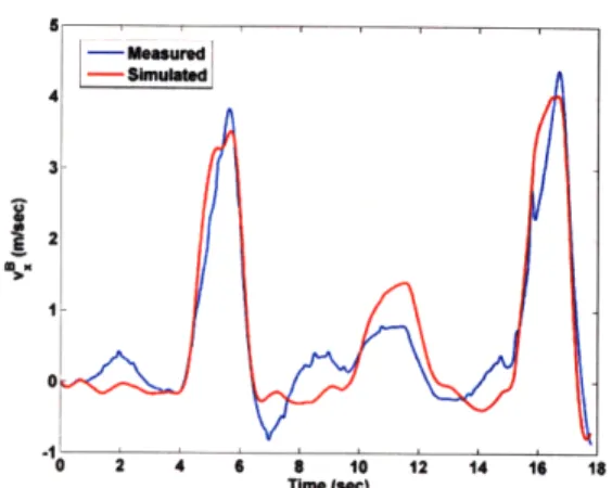
The following results compare the measured and simulated states for two types of ma-neuvers. These maneuvers include sinusoidal inertial y-velocity commands in hover causing the vehicle to oscillate about the body y-axis and the full transition to level-flight and back to hover which uses the controller outlined in Chapter 3. The simula-tion is given the initial condisimula-tions of each state and the input to each of the control surfaces for processing. In order to provide manual control of the vehicle, an ex-ternal joystick is programmed that commands desired velocity in both the x and y-inertial frame. This allows the user to define a suitable starting position within the

constrained environment. A trigger switch, when executed, commands the desired autonomous maneuver. For each executed maneuver, the body velocities and rota-tional rate are of interest and are compared in the following plots. It is important to note that the modeling is done primarily to support the transition maneuver on the body x and z forces and the y-axis moment.

Sinusoidal Velocity Inputs

For this test, a sinusoidal input to the y-inertial velocity is commanded and used to determine the accuracy in hover and high angles-of-attack with slight transition to level-flight mode properties. The sinusoidal input is commanded as

I = 2 sin(7t).

This is an important test that is used to determine the accuracy of the model that was accomplished through the prop-hang test. It verifies how well the propeller downwash velocity is modeled as well as moments created by control surface actuation. Since the aircraft is primarily in a hover position, the body x-axis is mainly testing the modeling of the thrust force created by the propeller shown in Figure 2-12(a). Due to inaccuracies in the power supply and un-modeled motor lag dynamics, slight deviations are present. Most of the sinusoidal command can be seen in Figure 2-12(e). For this inertial velocity command, the body z-velocity will mainly experience drag at a very high angle-of-attack. Most of the moment is generated about the y-body axis which is evident in Figure 2-12(d). Deviations occur after peak inputs which are distinctly due to the quasi-steady state modeling.

Transition to Hover and Back

The main test is to compare the output during a transition from hover to level-flight and back to hover. To obtain this desired maneuver, an exponential decaying y-velocity,

0.6 VOA 0.2 0 20 5 10 20 Time (ec)

(a) Body x velocity which for this test is mostly thrust 0.8 0 3-Simulated o 0.2

A

J

rate compensating for

pro-(c) Body y velocity

10

Time (sec)

(d) Pitch rotational rate

z velocity which mainly experiences (f) Yaw rotational rate

Figure 2-12: System Identification: compared state outputs for the sinusoidal velocity

test

(e) Body drag

is commanded due to the spatial limitation of a horizontal distance of 9.5 meters. This command allowed the vehicle to transition from hover to steady-level flight as can be seen in Figure 2-13.

A comparison of the measured to simulated state data is provided in Figure 2-14. This data shows two takes of this maneuver which is apparent by the two large spikes in Figure 2-14(a). Larger deviations are noticeable and are due to the very quick control surface actuation necessary to perform the transitions. The largest deviation in force is shown in Figure 2-14(e) at the point where the aircraft transitions from level to hover flight regimes. At this point the aircraft is essentially performing a skid stop, moving considerably quick at this high angle-of-attack. Flow separation makes the drag calculation a bit more obscure and the model over predicts these forces. However, trends in the data are similar and show that even with some un-modeled dynamics, the model can predict a response sufficiently well.

3-9

bt

*:

1-₂

0

0 2 4 6 8 10 12 14 16 18

Time (ec)

(a) Body x velocity which experiences both drag and lifting forces

- Measured 0.2 -0. -0.6 -0.8-0 2 4 6 8 10 12 14 16 18 Time (sc) (c) Body y velocity 4 S - Simulatedi 2 2 8 10 Time (sec)

(e) Body z velocity which experiences both drag and lifting forces

(b) Roll rotational rate

-0 2 4 6 8 10 12 14 16 18

Time (sec)

(d) Pitch rotational rate contributing all the mo-ment needed to perform the transition

4v

-Time (ec)

(f) Yaw rotational rate

Figure 2-14: System Identification: compared state outputs for the hover to transition test

Chapter 3

Quaternion Based Control

3.1

Introduction

One of the most recognizable issues when designing a controller to perform aggressive flight maneuvers is the concern over which attitude descriptor to use. The stan-dard aerodynamic Euler angles suffer from singularity problems due to gimbal lock, a point in which a degree of freedom is lost. Therefore, other descriptors such as the quaternion and direction cosine matrix (DCM) are used, each with its own distinct advantage. In Chapter 2, the aircraft model was pieced together using a DCM, an orthogonal matrix whose inverse (and consequently the transpose due to the proper-ties of orthogonal matrices) represents the reverse transformation. One of the caveats of using this descriptor is the amount of computation that must be done in order to complete a single transformation, 9 multiplications and 6 summations per transforma-tion. Quaternion descriptors are less computationally intensive and, in this chapter, the use of a quaternion based controller is presented. Figure 3-1 shows the controller's inner and outer loop architecture. Section 3.2 explains how the inner loop stabilizes the attitude of the aircraft based on a nominal desired quaternion and rotational rate by utilizing many of the properties of quaternion mathematics. The inner controller also regulates the amount of thrust necessary to perform a maneuver based on veloc-ity errors while attempting to maintain its vertical position. The velocveloc-ity controller provides the inner loop with an updated desired quaternion based on the error

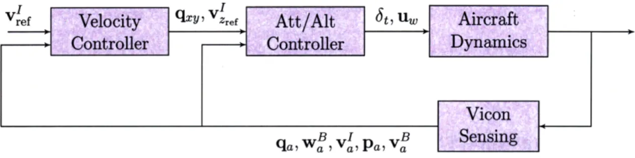
be-Figure 3-1: Quaternion-based control system architecture

tween commanded and measured velocity, and also an update on vertical position loss. Again, the RAVEN testbed is used to provide all the state data necessary to close the loop.

3.1.1

Notation

Quaternions are defined using a four-element vector, q = (qo, q, q, z) = (qo, q),

representing a rotation in R3 space. The basic algebraic form of a quaternion is:

q = qo + qxi + qyj + qzk. (3.1)

These four elements have the unit magnitude property in the usual 3-dimensional vec-tor space. The symbol 0 implies a quaternion multiplication while q* is the quaternion conjugate defined as

q* = qo - qxi - qyj - qzk. (3.2)

The subscripts in this chapter follow the same nomenclature presented at the begin-ning of Chapter 2.

3.2

Inner Attitude Loop

This inner attitude loop is a PD controller based on a desired attitude quaternion error and body rates [15]. The controller is developed to maintain a nominal prop-hang orientation. For the sake of avoiding confusion of multiple frame transformations, a

hover orientation is define as

1.0

qref 0.0 (3.3)

0.0

0.0

In this orientation, the body z and x-axes are aligned with the inertial y and z-axes respectively. RAVEN provides the measured vehicle quaternion orientation data, and the error deviated from the reference quaternion is calculated using quaternion multiplication as

qe = ref q * (3.4)

where (.)* represents the quaternion conjugate. The individual rotational error about the reference quaternion is found by calculating the axis angle interpretation, defined by:

[axis, angle] = a , 'Yrotation

To find the rotational error for an individual axis, the total rotation error must first be defined by

rotation = 2 cos(qeo)

and the axis vector error as

a, = sin(yrotation/2)

e,

The axis angle vector is a unit vector by definition and multiplying each component by the total error rotation yields the individual axis errors given by

e _az

8e rotation ax

V e ay

Each one of these axis angular errors are defined from the desired attitude. It is important to note that in this orientation, the commonly viewed roll error, labeled

¢e, is about the axis. This is consistent with having the body x and inertial

z-axes aligned, and similar arguments are made for the other axis errors. The control command that maintain a hover orientation is defined as u,

Kp6a 0 0

e

U = 0 Kp6e 0 Oe + 0 Kd6e 0 w (3.5)

0 0 Kp, Oe 0 0 Kd,

which is a PD controller on attitude.

3.3

Outer Velocity Loop

The outer velocity loop is a PI controller on the velocity error in the inertial frame. This control command manipulates the desired quaternion to produce an attitude in the direction of decreasing velocity error. One of the goals in performing this transition maneuver is to maintain a desired altitude, therefore the controller will limit the amount of control authority as a function of altitude loss.

In order to redefine a new attitude, a transformation that manipulates the desired quaternion based on the error of the inertial velocity command is developed. Since the objective of this controller is to translate the aircraft in the inertial x and y di-rection while maintaining altitude, errors between commanded and measured inertial velocities will be used to affect the transformation. Start by defining the inertial

velocity error as

Vxe

[Vxd

vye = Yd - VY (3.6)

Vze Vzd - VzaJ

and inertial z-error as

Ze =Zd - Za. (3.7)

These errors can be used to define the final quaternion transformation 1.0

KpyveZVye + Kiyvel

f

q9y

=

(3.8)

Kpvel VXe + Ki ve f vXedt + Kpzsign(vxa)ze _{+ Kzsign(vXa)vz}

0.0

So from an intuitive perspective, to obtain a desired velocity in the inertial y-direction, a rotation about the inertial x (second element of qx) must be performed. The same reasoning is applied to the third element of qxy. The vehicle will need to change its attitude, which is proportional to the error, but if a loss of altitude is sensed, the velocity controller will attenuate the attitude command based on the inertial z-velocity and position error which are the final two terms in Equation (3.8). Note that this is not a unit quaternion and needs to be normalized before performing quaternion multiplication. Quaternion multiplication is a transformation [23], so the new desired quaternion based on an inertial velocity command is

qa = qdef 0 qy. (3.9)

This new desired quaternion is what the inner loop will now act on, deflecting control surfaces in a manner that decreases the inertial velocity error and maintains altitude.

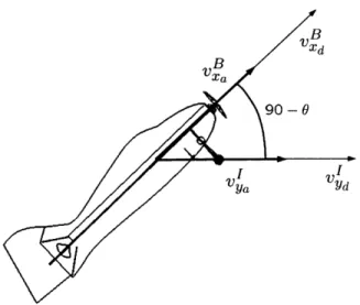
B Vxd B Xa I Ya I Yd

Figure 3-2: Vector description of additional body x-velocity necessary to obtain de-sired inertial velocity

3.4

Thrust Controller

The thrust controller is a PID controller with a feed-forward weight component, whose main functionality is to maintain a desired altitude. When performing the transition, modifications are used in an attempt to account for anticipated altitude loss and aerodynamic gain. One such modification is an adjustment of the feed-forward weight term as a function of 0, an angle measured from the vertical. The other is attempting to increase the body x velocity in order to decrease the inertial velocity errors. Figure 3-2 shows the velocity vector depiction of this modification, which is given by

VI

AvB Ye if 0 > 300 (3.10)

x sin 0

Notice that as 0 increases to 900, the error in the body velocity equals the error in the inertial frame. The complete control law is given as

mg + K z + Ki6 f zIdt - KdV v if 0 > 300

6t = +t - z (3.11)

In hover the controller is a regular PID controller where v, provides the damping in the body frame. As the translation occurs, the modifications regulate the thrust, attempting to maintain the desired altitude and decrease the inertial velocity errors.

3.5

Results

3.5.1

Simulation

A simulation was developed to test the capabilities of the controller and to find the gains necessary to stabilize the system in a prop-hang orientation. To make the model more realistic, an ensemble of state data was taken to determine the mean and variance of the measurement noise. Saturators were added to the control actuators as well as time delays to limit their performance to a realistic range. Table 3.1 shows the gains that are used in the model as well as on the actual flight hardware.

Table 3.1: Simulation quaternion attitude loop gains Gains Aileron Elevator Rudder Thrust

Kp 1.4 2.0 1.7 0.8

Ki 0.0 0.0 0.0 0.2

Kd 0.2 0.25 0.1 0.33

3.5.2

Decoupled Roll Control

Since the velocity commands are given in an inertial frame, the controller has an additive feature that will track the velocity commands decoupled from the aircraft roll orientation. For instance, if the aircraft is at a roll angle that does not correspond to a single control surface deflection (e.g. elevator) to obtain the desired velocity, the controller will couple the commands from the elevator and rudder.

To produce this roll decoupling feature, a transformation from the reference to the current roll angle quaternion must be calculated. A problem arises since the measurement of the current roll angle is not accurate, due to gimbal lock, and therefore

an intermediate derivation must be computed. This derivation involves the same computation as the inner loop controller but only the roll information is used.

To proceed, transform the measured quaternion into this new intermediate orien-tation (qint) by defining

qint = qa 0 qref. (3.12)

The conversion from quaternion to roll Euler angle is found by

= arctan 2(qontqXint+ qYintqzit) (3.13)

1 - 2(qxint + qyint)

which is the roll angle defined from hover.

Since the desired quaternion (Eq. 3.3) is a transformation in itself (level-flight to hover), the roll transformation has to take place on the z-element of the quacernion, therefore defining the roll decoupling transformation as

cos ₂ 0.0

qron = (3.14)

0.0 sin 0

which is a unit quaternion by definition. Now Equation (3.9) can be re-written as

_ref (3.15)

qd = qdf 0 roll qxy. (3.15)

This redefined desired quaternion is now independent of the roll angle of the aircraft. With this decoupling feature, a roll rate controller can be used to perform the rolling

hover. This is a PI controller on the roll rate error defined as

3

a = KpronllWxerr + Kiron Wxerrdt (3.16)

where