An Accurate Analytical Framework for Computing
Fault-tolerance Thresholds Using the [[7,1,3]]
Quantum Code
by
Andrew J. Morten
Submitted to the Department of Physics
in partial fulfillment of the requirements for the degree of
Bachelor of Science in Physics
at the
MASSACHUSETTS INSTITUTE OF TECHNOLOGY
September 2005
(© Massachusetts Institute of Technology 2005
All rights reserved.Author
... ...
-(7Certified
by...
epartment of Physics August 26, 2005 . _-. .Is....ac ChuangIsaac Chuang
Associate Professor, Department of Physics
Thesis Supervisor
Accepted by...
... C...
...-
.
...
David E. Pritchard
Senior Thesis Coordinator, Department of Physics
..n, s. IVvsE A4. .$v!. F- ... MASSACHUSETTS INSTtTE OF TECHNOLOGY JAN 3 0 2006 LIBRARIESAn Accurate Analytical Framework for Computing
Fault-tolerance Thresholds Using the [[7,1,3]] Quantum Code
by
Andrew J. Morten
Submitted to the Department of Physics on August 26, 2005, in partial fulfillment of the
requirements for the degree of
Bachelor of Science in Physics
Abstract
In studies of the threshold for fault-tolerant quantum error-correction, it is generally assumed that the noise channel at all levels of error-correction is the depolarizing channel. The effects of this assumption on the threshold result are unknown. We address this problem by calculating the effective noise channel at all levels of error-correction specifically for the Steane [[7,1,3]] code, and we recalculate the threshold using the new noise channels. We present a detailed analytical framework for these calculations and run numerical simulations for comparison. We find that only X and Z failures occur with significant probability in the effective noise channel at higher levels of error-correction. We calculate that when changes in the noise channel are accounted for, the value of the threshold for the Steane [[7,1,3]] code increases by about 30 percent, from .00030 to .00039, when memory failures occur with one tenth the probability of all other failures. Furthermore, our analytical model provides a framework for calculating thresholds for systems where the initial noise channel is very different from the depolarizing channel, such as is the case for ion trap quantum
computation.
Thesis Supervisor: Isaac Chuang
Acknowledgments
The length of my acknowledgements list is in indirect proportion to my gratitude to-ward those acknowledged. I would not have completed this work without the support of Prof. Isaac Chuang and Andrew Cross. I would like to thank Prof. Isaac Chuang for introducing me to the problem and for providing me an opportunity to work with his group at the Media Lab. I learned a great deal from interactions with his research group, especially with Andrew Cross. I cannot thank Andrew Cross enough - for providing my with a chunk of code that eventually became my QEC simulator, for many useful and eye-opening conversations about quantum error-correction whenever and wherever I needed them, for letting me use what would otherwise have been his computing cycles, and for his support during the final writing of this thesis.
Contents
1 Introduction 1.1 Outline . 2 Background 2.1 Quantum Computation . 2.1.1 Network Model. 2.1.2 Stabilizer Formalism ...2.2 Quantum Error Correction ...
2.2.1 Quantum Noise Model ... 2.2.2 Classical Error Correction . 2.2.3 CSS Codes and the [[7,1,3]] Code 2.2.4 Circuit Construction ... 2.2.5 Fault Tolerant Thresholds ....
3 The Model
3.1 Replacement Rule ... 3.2 Error Correction Circuit ... 3.3 Modeling Choices ...
4 Analytical Approximation
4.1 Analysis Overview ...
4.2 Notation ...
4.2.1 The Error Correction Network ...
17 18 19 20 20 21 23 23 25 27 29 34 37 37 39 41 45 45 46 46
...
...
...
I ....
...
...
...
...
...
...
...
...
4.2.2 Failure Rates 4.2.3 Probabilities . 4.3 Alpha ...
4.4 Incoming Errors on Data 4.5 Noise Channels ...
4.5.1 Single Qubit Gate. 4.5.2 Two Qubit Gate 4.5.3 Measurement 4.5.4 Preparation . 4.6 Threshold ... 5 Results 5.1 Numerical Simulations 5.2 Alpha ...
5.3 Incoming Errors on Data 5.4 Noise Channels ... 5.5 Threshold.
6 Conclusions and Further Directions A Probabilities
B Counting Tables for Failure Rate Estimates C Error Correction Circuits
D ARQ Code Generator for [[7,1,3]] Quantum Code E Sample ARQ Code
47 48 50 54 60 60 64 65 66 66 69 69 70 73 74 74 83 85 87 91 95 117
...
...
...
...
...
...
...
...
...
...
...
...
...
...
...
List of Figures
2-1 This is the circuit for the preparation network, G. It prepares the logical zero state, 0)L. It is used in the error-correction circuit (see
Section 3.2) to prepare ancilla qubits in the state 0I)L£ ... 30 2-2 This circuit measures the operator Z on the qubit Iqd) and projects Iqd)
into an eigenstate of Z with the measured eigenvalue. ... 31 2-3 The verification network V checks for X errors on the state 0I)L and
gives four zero measurement results if no X errors are detected. ... . 32 2-4 The syndrome extraction network S consists of three time steps. The
above network is the syndrome extraction for Z error correction. The syndrome extraction network for X error correction is the same, except with each cnot replaced by cz. ... 33
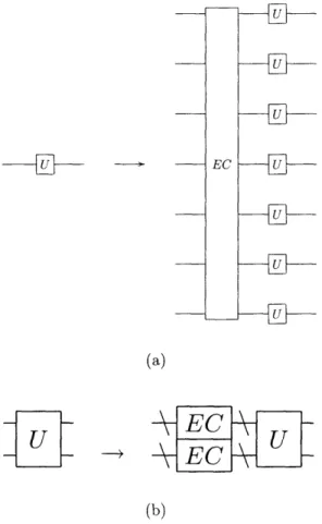
3-1 (a) The replacement rule for a single qubit gate. (b) The replacement
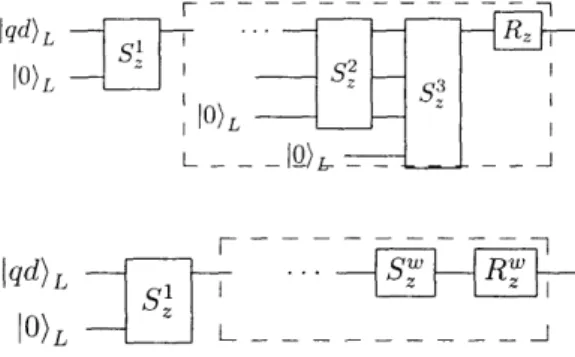
rule for a two qubit gate. ... 38 3-2 The error correction routine finds and corrects errors on the seven data
qubits in the logical state qd)L with the aid of multiple copies of ancilla qubits in the logical zero state 0)L. The second half of the circuit is on of two possibilities, depending on whether the first syndrome extraction SJ was zero or non-zero. If the syndrome is non-zero, then two more syndromes are collected (middle circuit), but if the syndrome is zero, no more syndromes are collected and the data qubits wait (righmost circuit) during the syndrome extraction circuit acting on other qubits. 39
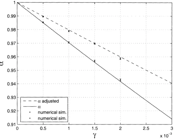
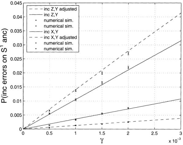
5-1 This is a graph for , the probability that the verification network passes, versus the failure rate y Y1 = /2 m = p = 1 0yw. It is plotted twice: once assuming the depolarizing channel (solid line), and once assuming the effective channel that we calculate in Section 5.4 to be the higher level noise channel ("adjusted" dashed line). ... 71 5-2 This is a graph of the probabilities of incoming errors on the ancilla
coming into S1 versus the failure rate -y1 = -y2 = /m = Yp = 10"/w The probabilities are plotted twice: once assuming the depolarizing channel (solid lines), and once assuming the effective channel that we calculate in Section 5.4 to be the higher level noise channel ("adjusted" dashed lines). The legend indicates the the order of the plotted prob-abilities as they appear in the graph from top to bottom. ... 72 5-3 This is a graph of the probabilities of incoming X, Y, and Z errors
into Z error-correction: P, pY, and Pz. They are plotted against the failure rate y - 1 = /2 = m, % = 10yw The probabilities are plotted twice: once assuming the depolarizing channel (solid lines), and once assuming the effective channel that we calculate in Section 5.4 to be the higher level noise channel (dashed lines). The legend indicates the the order of the plotted probabilities as they appear in the graph from top to bottom. ... 78 5-4 The is a graph the effective noise channel (the separate probabilities of
X, Y, and Z errors) at level + 1 versus the failure rate y -yl = y2 = y, = p = 10oy at level . The probabilities are plotted twice: once assuming the depolarizing channel, and once assuming the effective channel that we calculate in Section 5.4 to be the higher level noise channel. We also plot the probability of an X or Y error (denoted X,Y error) and compare to numerical simulation. The legend indicates the the order of the plotted probabilities as they appear in the graph from
5-5 This is a graph of the threshold for the Steane [[7,1,3]] code. The horizontal axis is Yelse -= 1 = % = = /ym and the vertical axis is U,. The solid line is the threshold result assuming depolarizing noise at all levels of error-correction. The dashed line is the threshold result when the noise channel changes according to our analytical model. Along the line yelse = 10-yw, the threshold increases from 3.0 x 10⁻⁴ to 3.9 x 10- 4
when we take into consideration the changing noise channel. ... 80
5-6 This is a graph of the failure rates at level + 1 in terms of the failure rate - 1 = 2 = am = yp = 10
Yvw
at level e. The probabilities are plotted twice: once assuming the depolarizing channel, and once assuming the effective channel that we calculate in Section 5.4 to be the higher level noise channel. The legend indicates the the order of the plotted probabilities as they appear in the graph from top to bottom. 81C-1 The error correction routine finds and corrects errors on the seven data qubits in the logical state qd)L with the aid of multiple copies of ancilla qubits in the logical zero state 0)L. The second half of the circuit is on of two possibilities, depending on whether the first syndrome extraction Sz was zero or non-zero. If the syndrome is non-zero, then two more syndromes are collected (middle circuit), but if the syndrome is zero, no more syndromes are collected and the data qubits wait (righmost circuit) during the syndrome extraction circuit acting on other qubits. 92
C-2 This is the circuit for the preparation network, G. It prepares the
logical zero state, 0)L. It is used in the error-correction circuit (see
Section 3.2) to prepare ancilla qubits in the state
I0)L.
... 92C-3 The verification network V checks for X errors on the state 0)L and gives four zero measurement results if no X errors are detected. ... 93
C-4 The syndrome extraction network S consists of three time steps. The above network is the syndrome extraction for Z error correction. The syndrome extraction network for X error correction is the same, except with each cnot replaced by cz ... 94
List of Tables
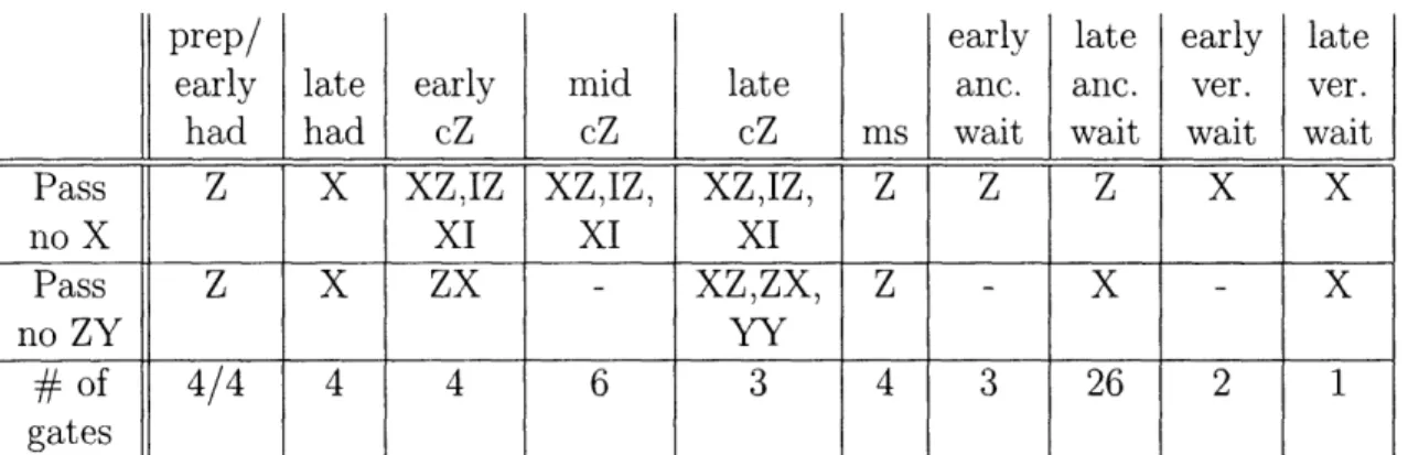
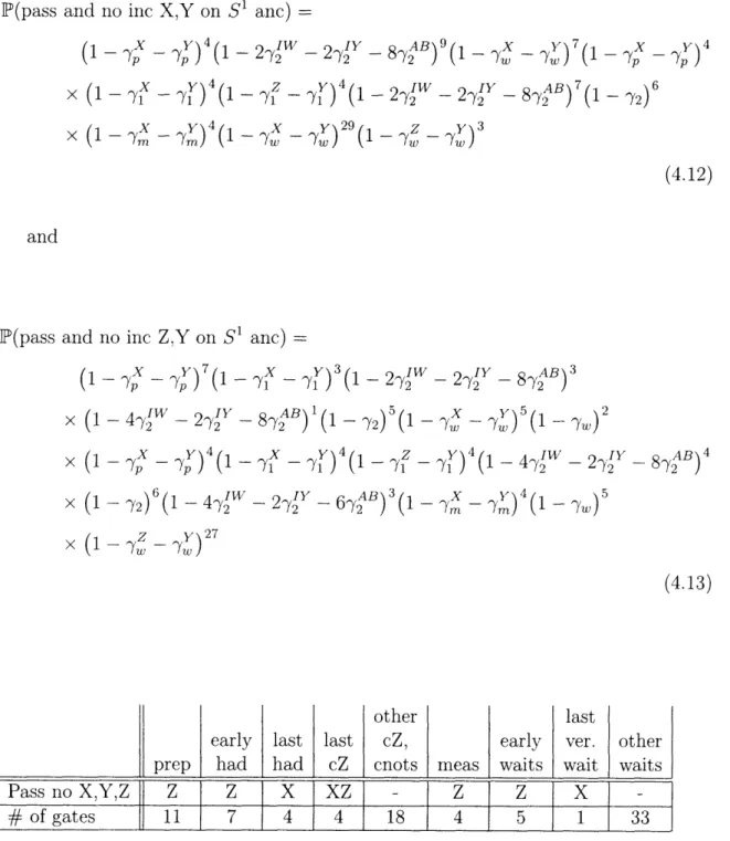
4.1 This table lists the failures in the G network that lead to good outcomes for the probabilities P(pass and no inc X,Y on S1 anc) and IP(pass and no inc Z,Y on S1 anc). The bot. prep. gates are the preparation gates followed by Hadamards, and the top prep. gates are the ones that are not followed by Hadamards. The early cnot gates are the three in the second time step, the mid. cnot gate is the cnot gate in the third time step that still acts on a 10), while the late cnot gates include all others. 52 4.2 This table lists the failures in the V' network that lead to good
out-comes for the probability IP(pass and no inc X,Y on S1 anc) and IP(pass
and no inc Z,Y on S1 anc). ms is short for measurement gate. .... 52
4.3 This table lists the failures in the G and V1 networks that lead to good outcomes for the probabilities P(pass and no inc X,Y,Z on S1 anc). The last cZ gates are the cZ gates that are the last to act on each verification qubit ... ... ... 53 4.4 This table lists all pairs of errors that cause a logical X or Y error. The
columns indicate the location of the first error and the rows indicate the location of the second error. The column and row labeled "inc" correspond to incoming errors on S1 ancilla. ... . 63
4.5 This table lists all errors that cause a logical X or Y failure, given either an incoming X error (first row) or an incoming Y error (second row). See Appendix B for an explanation of the designation "s". .... 64
5.1 This table shows the behavior of the noise channels just below
thresh-old. Rows 1-4 give the noise channels for successive levels of error-correction in our model. Rows 5-8 give the noise channels for successive
levels of error-correction assuming that the noise channel is depolariz-ing at each level. ... 76 5.2 This table is the same as Table 5.1, except only the full failure rate for
each type of gate is presented. ... .. 76 A.1 All probabilities needed for the calculation of Pz , YPZZPX, z pY
and PZ given in Section 4.4 and the calculations of the failure rates in Section 4.5 can bee looked up in this table. In the top section, the label W can be replaced by either X or Z. The gate U2 is taken to be
a cz gate. ... 86 B.1 This table lists all pairs of errors that cause a logical X or Y error. The
columns indicate the location of the first error and the rows indicate the location of the second error. The column and row labeled "inc" correspond to incoming errors on the S~ ancilla. ... 88
B.2 This table lists all errors that cause a logical X or Y failure, given
either an incoming X error (first row) or an incoming Y error (second row). The column labeled "inc" corresponds to an incoming error on the S1 ancilla. ... 88 B.3 This table lists all pairs of errors that cause a logical Z or Y error. The
columns indicate the location of the first error and the rows indicate the location of the second error. The column and row labeled "inc" correspond to incoming errors on the S' ancilla. ... 89 B.4 This table lists all errors that cause a logical Z or Y failure, given either
an incoming Z error (first row) or an incoming Y error (second row). 89 B.5 This table lists all pairs of errors that cause a logical Y error. The
columns indicate the location of the first error and the rows indicate the location of the second error. ... 90
B.6 This table lists all errors that cause a logical Y failure given an incoming
Y error. . . . .. ... 90
E.1 The classical instructions defined in ARQ. ... 118
E.2 The quantum instructions defined in ARQ. ... 119
Chapter 1
Introduction
Quantum fault-tolerance is the key to a successful physical realization of a large-scale quantum computation. Using concatenated quantum error-correcting codes [17,
18, 10], it has been shown that as long as the noise in a system is below a certain threshold, arbitrarily long fault-tolerant quantum computations can be performed[2, 9, 11, 13. 8, 3]. The Steane [[7,1,3]] is the most promising among the small quantum error-correction codes. Many studies of the threshold for the Steane [[7,1,3]] code
have been carried out[22, 14, 2, 19, 16, 21].
Previous estimates of the threshold for the Steane [[7,1,3]] code have assumed that the noise channel is the depolarizing noise channel at all levels of concatenation. In the depolarizing channel, the three types of errors X, Y, and Z occur with equal
probability. In a concatenated code error-correction procedure, every level of
con-catenation has its own effective noise channel, which can be very different from the depolarizing channel. No detailed study of the effects of changes in the noise channel on the threshold has been done.
In this thesis we answer the following two questions: What is the effective noise channel at different levels of concatenation of the Steane [[7,1,3]] code? More im-portantly, how does the estimate of the threshold change when the different noise channels are taken into account?
We answer these two questions using an analytical model. Additionally, we con-duct simulations to verify the accuracy of our model. Because our analytical model
must distinguish between X, Y, and Z errors, it is necessarily more detailed than the models used for previous estimates of the threshold for the Steane [[7,1,3]] code. We contribute to the ongoing study of the Steane [[7,1,3]] code by providing this new, richer analytical model.
1.1 Outline
In the next Chapter of this thesis, we present some background in quantum computa-tion and quantum error correccomputa-tion that will be used in later seccomputa-tions. We present only what is needed for an understanding of the later sections, and we introduce concepts in a way that assumes only some familiarity with quantum mechanics and classical
computation.
In Chapter 3 we describe the model we use to calculate the threshold for the Steane [[7,1,3]] code. Modeling choices include the quantum circuit used for error-correction, the replacement rule that prescribes how to construct circuits for concatenated codes,
and the noise model.
The main achievement of this thesis is the analytical model which we present in Chapter 4, along with the tables in Appendices A and B. This very detailed model is used to determine the noise channel at all levels of concatenation and the resulting threshold.
We then make predictions using our analytical model and compare a subset of the predictions to numerical simulation results in Chapter 5. We wrote code that generates quantum computer assembly code instructions for the Steane [[7,1,3]] code that were input to a program called ARQ, a quantum computer simulator. The ARQ code generator and some sample output ARQ code are given in Appendices D and E. In the last Chapter we review our results and discuss limitations of and possible improvements to our analytical model.
Chapter 2
Background
In Section 2.1 we introduce the network model of quantum computation and the stabilizer formalism. The network model is the quantum mechanical generalization of the theory of classical circuits. In the network model, the classical bits 0 and 1 get replaced by the quantum states 10) and 1), and classical logic gates get replaced by unitary transformations. We use the network model to represent our quantum error-correction routine. The stabilizer formalism of quantum mechanics has to do with representing the state of a system with a complete set of commuting observ-ables. Stabilizer circuits and the propagation of errors through them have an efficient mathematical description. We will use the stabilizer formalism in describing how to construct our error-correction circuits, why they work, and how we can simulate them
efficiently on a classical computer.
In Section 2.2 we introduce quantum error correction. Because of the properties of quantum measurement, quantum errors can by "digitized," so they appear as bit or phase flips on a subset of qubits. Cleverly used classical error-correcting codes can then be applied to correct these errors. First we introduce quantum noise and the noise model used throughout the analysis. Next we explain the theory behind the Steane [[7,1,3]] error-correcting code by discussing classical error correction and a group of quantum error-correction codes, called CSS codes. After that we explain how to use the stabilizer formalism to construct and understand the quantum circuits for the [[7,1,3]] code. Finally, we explain the threshold result for quantum computation
and summarize previous work on the Steane [[7,1,3]] code.
2.1 Quantum Computation
We give a general overview of the network model of quantum computation and the stabilizer formalism. See [12] for much of the material we present here.
2.1.1
Network Model
In this thesis we restrict ourselves to the network model of quantum computation. Other models for quantum computation exist, such as cluster states [15] and adia-batic evolution [7], but the network model is suitable for our present study of the concatenation of the Steane [[7,1,3]] code. These other models have been shown to be equivalent to the network model.
The theory of quantum computation in the network model [6] is the quantum mechanical generalization of the theory of classical circuits. In the classical circuit model, a circuit of logical gates acts on input bits to produce output bits. If the set of logical gates is universal, then any possible classical computation can be achieved in the classical circuit model (more precisely, any function f Zm -, Z can be evaluated). In the quantum network model, a "circuit" of unitary transformations
(gates) acts on input quantum states to produce output quantum states. If the set of
unitary gates is universal, then any possible quantum computation can be achieved in the quantum network model (more precisely, any specified state can be created with arbitrary precision).
The inputs and outputs in the quantum network model are quantum states. The Hilbert space of these states is a tensor product of two-level systems, and the eigen-states of each two-level system are written as 10) and I1). The eigen-states in these two-level systems are called quantum bits, or qubits, in reference to their classical analogue. A physical example of a qubit would be a spin 1/2 particle with 10) = I) and I) -= IT).
The gates in a quantum circuit are all unitary transformations, as required by the postulates of quantum mechanics. In our quantum error correction circuit, we
assume that a few elementary quantum gates are available to the quantum computer: the identity I; the Pauli gates X, Y, and Z; the Hadamard gate H; cnot (control-X), cz (control-Z), and the Toffoli gate. We list the definitions of the identity gate, Pauli gates, and the Hadamard gate here in matrix representation in the {10), II)} basis:
I =
, H=
(2.1)
I 1 H V2_ I (2.1)
X 1i = , (2.2)
10 i 0 0 -1
The cnot and cz gates act on two qubits: a control qubit and a target qubit. They apply the X and Z gates, respectively, to the target qubit when the control qubit is 11), and do nothing when the control qubit is 10). This defines their behavior on the basis states {100), 10) , 01) , 11)}, so their behavior has been fully specified on all input two qubit states.
The Toffoli gate is a three qubit gate that acts as a cnot with two control qubits that must both be I1) for the X to be applied to the target.
A set of universal quantum gates is for quantum computation in the network model is {X,Y,Z,H,cnot,cz,Toffoli}. This is not a minimal set; these are the six fundamental gates that we assume can be carried out by the quantum computer in our model.
2.1.2 Stabilizer Formalism
We use the stabilizer formalism because it offers a compact representation of a cer-tain subspace of quantum states. It allows us to simulate quantum error correction networks efficiently on a classical computer.
A stabilizer circuit is a circuit that consists only of gates that are in the normalizer
of the Pauli group, and single qubit measurements. Included in this list of gates are the X, Y, Z, cnot, and cz gates. The only gate in our universal family of gates not included in this list is the Toffoli gate. The Gottesmann-Knill Theorem [8] states
that any stabilizer circuit can be simulated efficiently on a classical computer, as long as the initial state is a stabilizer state.. The error-correction circuit we use for the Steane [[7,1,3]] code is a stabilizer circuit.
If the quantum state ) satisfies U IV) =
4)
for some unitary gate U, we say that U stabilizes I). For example, the state 10) is stabilized by the Pauli operator Z, and the state H 10) = (10) + 1))/I 2 is stabilized by the Pauli operator X. In fact, the states in these two examples are the unique states (up to a global phase) that arestabilized by their respective gates.
The Pauli group G1 on one qubit is defined to consist of the identity (I), the three Pauli operators (X,Y,Z), and all operators created by multiplying the above operators by ±1 or i. The Pauli group G, on n qubits is defined to consist of all n-fold tensor
products of elements of G1.
A vector space V of quantum states is stabilized by a subgroup S of the Pauli
group G, on n qubits if every state in V is stabilized by every operator in S. Any
subset of S that generates S is called a set of stabilizer generators for V. If V contains a single quantum state with m qubits, then a set of m independent stabilizer generators uniquely defines the state (up to phase).
In our numerical simulations, we keep track of the stabilizer generators of the quantum system, rather than the state itself. We always keep track of the minimum number of stabilizer generators such that the state is uniquely specified (up to a phase). The stabilizer of the quantum system evolves as follows. If the current state is
41)
with stabilizer g, then after a unitary gate, the state becomes U ) = Ug I)) =UgUtU i), so the new stabilizer is UgUt. Because all of the gates we use in our
simulations (X, Y, Z, H, cnot, cz) are in the normalizer of the Pauli group Gn, we
always have UgUt E Gn. As long as the input state is stabilized by a subset of the
Pauli group, the evolving state is always stabilized by a subset of the Pauli group. Measurements also affect the stabilizer, but as long as the measurements are in the computational basis (that is, measurements of the operators X or Z), then the
stabilizer remains a subset of the Pauli group after measurement. We only use single qubit measurements in the computational basis in our circuits. So, we conclude that
we can efficiently simulate our error correction networks on a classical computer.
2.2 Quantum Error Correction
Quantum fault-tolerance is an essential ingredient for the physical realization of a quantum computer. Quantum fault-tolerance has three requirements: (1) we must be able to prepare encoded states, (2) we must correct errors on those states, and (3) we must control the spread of errors through our circuits.
In this section we present some background in quantum error correction. The purpose of this section is to provide the background in error correction needed by the rest of this thesis, so we limit the discussion to topics that will later be used.
In Section 2.2.1 we describe the quantum noise model, and how it can be inter-preted using a set of discrete errors. Then in Sections 2.2.2, and 2.2.3. we explain how these errors can be corrected using circuits that are themselves noisy. In Section 2.2.4 we explain how to construct the circuits for the Steane [[7,1,3]] error-correction code. We end with Section 2.2.5 explaining the threshold result and summarizing previous
work on the Steane [[7,1,3]] code.
2.2.1
Quantum Noise Model
Noise in a quantum network is not as simple as in the classical network, where the only possible error is a bit flip. In a noisy quantum network, there is a continuous spectrum of errors that can occur on a quantum state, because the quantum states are specified by two complex numbers (subject to normalization). Despite the continuous spectrum of errors, quantum error correction can be achieved by correcting only a small set of discrete errors [17, 18].
To represent quantum noise, we use the density operator formulation of quantum mechanics. In the density operator formulation, the state fiV) is represented by the outer product [¢)(¢[. If the state is unknown, but known to be 1i), 2), ... or I n)
with probabilities Pi, P2, .. P2n, respectively, then the associated density operator is n
P=
AP i)(Ki
kI
(2.3)
i=l
Such an operator is called a mixed state.
The application of the gate U to a mixed state p transforms the density operator into UpUt
The quantum noise model we use is called the depolarizing channel. In a depo-larizing channel, a single qubit is replaced by the completely mixed state 1/2 with probability p, and left unchanged with probability 1 - p. If the density operator of the single qubit state before the depolarizing channel is p, then the density operator
after the depolarizing channel is
I
D(p) = (1-p)p +
2 p1= (1 - p')p +
-(XpX
+ YpY + ZpZ),
(2.4)
3where we used the fact that for arbitrary p, I = (p + XpX + YpY + ZpZ)/2, and we
defined p' 3p/4.
Equation 2.4 can be interpreted (density operators can have multiple valid inter-pretations) as is the identity gate being applied with probability p' and each Pauli gate being applied with probability p'/3. In this interpretation we call the application of the Pauli gate X an X error, the application of the Pauli gate Y a Y error, and the application of the Pauli gate Z a Z error.
From now on, whenever we talk about quantum noise, we simply refer to the probability of X, Y, and Z errors.
Before we continue on to discuss error-correction, we explain how noise errors propagate through a circuit. This is very important to understanding how error correction works (and also why we need it).
When there is an X error on a single qubit state state
4V)),
then after the application of a Hadamard gate the new state is H(X [')) = Z(H4I)).
This is interpreted as a Zerror on the expected (without noise) state H Io). So, Hadamard gates propagate X errors to Z errors. They also propagate Z errors to X errors and Y errors to Y errors. We can similarly determine that cz gates propagate X errors on the control qubit to Z errors on the target qubit and propagate X errors on the target qubit to Z errors on the control qubit. Cnot gates propagate X errors on the control qubit to X errors on the target qubit but propagate Z errors on the target qubit to Z errors on the control qubit. These facts are used in the construction of the syndrome extraction networks designed in Section 2.2.4.
2.2.2 Classical Error Correction
Quantum noise must be corrected in order for quantum computations to be fault-tolerant. Quantum error correcting codes have been designed for this purpose. The Steane [[7,1,3]] quantum error-correcting code belongs to the collection of Calderbank-Shor-Steane (CSS) codes [4], which are based on classical linear codes. In this section we discuss classical linear codes, using the codes that lead to the [[7,1,3]] quantum code as ongoing examples. Much of the theory in this section and the next is borrowed
from [12].
The noise in classical error correction consists of bit flip errors: 0 becomes 1 with some probability, and 1 becomes 0 with some probability. A simple code for protecting against single bit flip errors is to represent the bit 0 by three bits 000 and the bit 1 by three bits 111. Then, if a single bit flip occurs, majority voting corrects the error.
In general, classical linear codes use n bits to store k bits of information. A linear code is specified by an n by k generator matrix G with entries in 72 (zeros and ones with addition modulo 2, i.e. binary numbers). The n bit codewords are created from the k bit words by the operation Gx, where x is the k bit word represented as a
column vector. For example, the generator matrix for the [[7,4,3]] Hamming code C1, G(C1) =
0 0 0
0 1 0 0 0 0 1 0 0 0 0 1 0 1 1 1 1 0 1 11101
(2.5)creates 7 bit codewords out of 4 bit words.
The [[7,4,3]] code is an [[n,k,d]] linear code, where d is the Hamming distance of the code. The distance of a code is the minimum distance between codewords, where the distance between two codewords is defined to be the number of bits at which the codewords differ. For example, the codewords generated by G are 0000000, 1010101,
0110011, 1100110, 0001111, 1011010, 0111100, 1101001, 1111111, 0101010, 1001100, 0011001, 1110000, 0100101, 1000011, and 0010110, where every pair of codewords
differs at at least three locations. Because the Hamming distance is three, if only
one bit of a codeword of [[7,4,3]] is flipped, we can determine which was the original
codeword. Codes can correct t (d - 1)/2 errors and detect d - 1 errors.
To determine which was the original codeword and how to correct for it, we use the parity check matrix H associated with G. The parity check matrix is an n - k by n matrix with linearly independent rows such that Hx = 0 for every codeword x, and it can be found directly from G. If a single error occurs on the jth bit of any codeword x, then parity check matrix reveals the error that occurred on the new
codeword x' = x + ej, using Hx' = H(x + ej) = 0 + Hej = Hey, where ej is column
vector of zeros with a one on the jth bit. The vectors Hej are called syndromes. The syndromes reveal the location of the bit flip errors and are unique because H has
The parity check matrix for the [[7,4,3]] code is
00011111
H(C) = 1 1 0 0 1 (2.6)
1 0 1 0 1 0 1
An interesting property of this code is that if an error occurs on the jth qubit, then
Hej is the binary representation of j.
Lastly, we describe an important classical linear code that can be constructed from any given classical linear code C: the dual of C, denoted C', is defined to consist of all codewords orthogonal to C. Equivalently, C' is defined by having the generator matrix HT. Dual codes are used in the creation of CSS codes, of which the Steane
[[7,1,3]] is a specific example.
2.2.3 CSS Codes and the [[7,1,3]] Code
A useful class of quantum error-correcting codes is the Calderbank-Shor-Steane [4] codes. CSS codes are based on classical linear codes and their duals. Given two
classical linear codes C1 and C2 of the type [n,kl] and [n,k2] such that C2 C C1 and
such that C1 and C2 correct t errors, we can construct an [[n,kl- k2]] quantum code
that corrects t errors. As part of our ongoing example of the Steane [[7,1,3]] code, we choose C1 as defined in the previous section, and C2 = C1. These codes are [7,4,3]
and [7,3,4] codes, respectively, so they combine to form a [[7,1,3]] quantum error-correction code, the Steane code. We describe what this quantum error-error-correction code is and how it works.
For every codeword x C1 we define a quantum state
Ix + C2)
E
I
+ y)
,
(2.7)
up to a normalization constant. Explicitly, the state (2.7) is either 1 10)L = (10000000) + 8 11010101) + 10110011) + 11100110) (2.8) + 0001111) + 11011010)+ 10111100) + 11101001)), or I1)L - (11111111) + 10101010) + 11001100)+ 10011001) + 1110000) + 0100101) + 1000011) + 0010110)), (2.9)
depending on the value of x E C1.
The eight states in the expression for 10)L are the codewords of the classical linear
code C2 c C1. The eight states in the expression for 11)L are the codewords in C1
that are not in C2.
If X errors are represented by the vector ex with bits set to one where X errors occur, and Z errors are represented by the vector ez with bits set to one where Z errors occur, then the quantum state in Equation 2.7 becomes
(2.10)
(_-)(
x+ y)e
zIx + y + ex)
yGC2Because Y = iXZ, Y errors are automatically corrected when X and Z errors are corrected.
The X error syndrome can be determined by using reversible quantum
computa-tion and ancilla to create the state
(2.11)
E
(-1)(x+Y)ezIX
+ y + ex) H(Cl)ex), Yt-U2ancilla
followed by measurement of the ancilla. The quantum circuit that achieves this is designed in Section 3.2. The syndrome is used to correct the bit flip errors by applying X gates on the appropriate qubits.
the data qubits, producing the state
E]
(-1)
'Z
z+ ez),
(2.12)
after some mathematical manipulations and using the definition of dual space C2. The syndrome (using H(C2) instead of H(C1)) is transferred to the ancilla and measured as in the X error correction. Note that by applying the Hadamard gates,
we turned Z errors into X errors. Since C1 = C52 in the case of the Steane [[7,1,3]] code,
we can use the same circuit for Z error correction as we did with X error correction, except Hadamards are applied to the data before and after Z the syndrome extraction.
2.2.4 Circuit Construction
In this section we use the theory of CSS codes to construct three circuits used in the Steane [[7,1,3]] error-correction code: G, the preparation network, which prepares the state 0I)L; V, the verification network, which verifies that there are no X errors on the qubits that make up
I0)L;
and S, the syndrome extraction network, which uses ancilla qubits to extract the classical error syndrome from the data qubits. The gateswe use are the same as in [21].
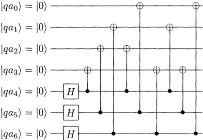
First, we construct the preparation network G, given in Figure 2-1. The prepa-ration network constructs the state 10)L, which is a superposition of all codewords defined by the generator matrix for C2,
G(C
2)
= 0 1 11 0 1
1 1 0
1 1 1
1 0 0
0 1 0
0 1
0 1 2 3, (2.13) 4 5 6where we have labeled the columns 0 through 6 to correspond to qubits qao) through qa6) in Figure 2-1. I _\ In\ i Ilqao = Iu Iqal) = 10) lqa2) = 10) lqa3) = 10) [qa4) = 10) qa5) = 10) qa6) = 10) --- f~~~ H H
_H
{a
JOI
I aU-IB I,-4
Figure 2-1: This is the circuit for the preparation network, G. It prepares the logical zero state, 10)L. It is used in the error-correction circuit (see Section 3.2) to prepare ancilla qubits in the state 10)L.
First we apply Hadamard gates to qubits 4, 5, and 6. This puts these three states into a superposition of all possible three bit words. Because rows 4, 5, and 6 in
G(C2) form a 3x3 identity matrix, the last three qubits in each seven qubit codeword
correspond to the three bits from which the codeword was derived using G(C2). This
makes determining what state to put the other qubits in quite easy. Reading off from the three columns of G(C2): if qubit 4 is I1) then qubits 1, 2, and 3 need to be
flipped; if qubit 5 is 1) then qubits 0, 2, and 3 need to be flipped; and if qubit 6 is II) then qubits 0, l1, and 3 need to be flipped. We apply nine cnot gates according
to the above three rules. Because G(C2) is a linear code and {001, 010, 100} forms a
basis for the input bits to G(C2), this circuit correctly constructs a superposition of
all codewords generated by G(C2).
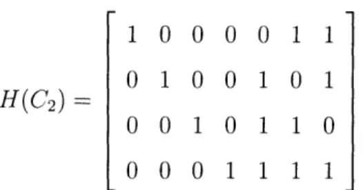
Next, using H(C 2) we construct the verification network shown in Figure 2-3. The
verification network verifies that that there are no X errors on the logical qubit
I0)L.
This is accomplished by measuring all stabilizer generators ofIO)L
that anti-commute with X errors. There are four such (independent) stabilizers, and a measurement result of 0 (meaning that the measured operator stabilizes the state) for all of them means that there is no X error. As can determined by reading off the rows of theI 11 I a)
:
It
.111 r a--J 0 4 P i b 1 : . > J1parity matrix H(C2),
H(C
2)
=1000011
0100101
0010110
0001111
(2.14)the stabilizer generators that anti-commute with X errors are
ZIIIIZZ, IZIIZIZ, IIZIZZI, and IIIZZZZ (2.15)
(the other three stabilizer generators are XIIIIXX, IXIIXIX, and IIXIXXI, which commute with X errors).
In general, to measure a single qubit (unitary, hermitian) operator M, you apply a Hadamard on the ancilla prepared in the state 10), followed by a control-M gate with control on the ancilla, followed by a Hadamard and measurement on the ancilla. This also projects the the measured qubits into the eigenspace of the measured eigenvalue. For example, the measurement of the operator Z is depicted in Figure 2-2.
Jqd)
Iqa)= 10) HF
Figure 2-2: This circuit measures the operator Z on the qubit qd) and projects qd) into an eigenstate of Z with the measured eigenvalue.
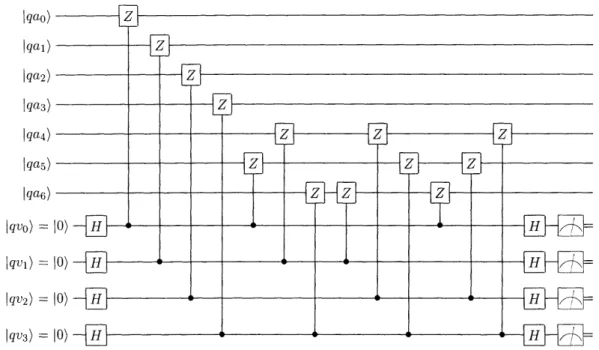
The circuit V in Figure 2-3 measures the four stabilizer generators that anti-commute with X errors. Each of the four verification qubits is used to measure on of the generators.
The matrix H(C1) is not the only parity check matrix for C1. Indeed, any matrix
formed by adding together rows of H(C1) would be equally valid. However, as
ex-plained in [20], putting H(C1) in the form (I,A) ensures that the derived verification
Iqao) Iqal) qa2) Iqa3) Iqa4) lqa5) I qa) Iqvo) = Iqvi) = Iqv2) = Jqv3) =
Figure 2-3: The verification network V checks for X errors on the state
IO)L
and givesfour zero measurement results if no X errors are detected.
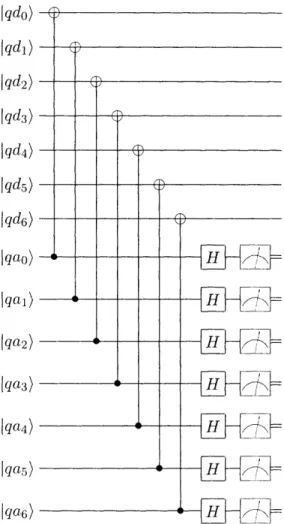
The third and last circuit we construct is the syndrome extraction network. There are two syndrome extraction networks: one that detects X errors, and one that detects Z errors. We explain how to construct the Z error syndrome extraction network, shown in Figure 2-4. The construction of the X error syndrome extraction is very similar.
First, a logical cnot gate is performed with the ancilla in the state 10)L as control and the logical data qubit as target. A logical cnot gate is just seven cnot gates acting transversally on the data and ancilla. Because the ancilla is in the state IO)L, the logical cnot gate does affect the logical data qubit. However, X errors on the ancilla propagate to X error on the qubits , and Z errors on the data qubits propagate to Z errors on the ancilla qubits.
Next, seven Hadamard gates are applied to the ancilla qubits, transforming Z
errors into X errors. This is followed by Pauli Z measurements of all the ancilla. If
there is no error, the result of the measurement will be in the code C1. The reason
for this is because the Hadamard gates are actually a logical Hadamard gate that transforms the state 10)L into the state (O) L + I1) L)/, which is a superposition of all of the codewords in C1. A classical syndrome extraction is done on the measurement
Iqdo) Jqdl) Iqd2) I qd3) Iqd4) Iqd5) Innu6/ lon} I-I r1'"u/ I -I-"/ too, u I fl.o') -e
-_
I'1 '- / I(JWn ' -J - -J 1-I (in" UI'0UM IaaM I UWT_ I I L1 I rL W - 1L i J UrTI L-iK] W L2 U" /i 1 I L 1' 1 'IE L
I i I ( Nj U -U I - LU 4/ {,~Figure 2-4: The syndrome extraction network S consists of three time steps. The above network is the syndrome extraction for Z error correction. The syndrome extraction network for X error correction is the same, except with each cnot replaced
by cz.
results to determine if any of the ancilla were flipped. If there is exactly one Z error on the data qubits coming into the the syndrome extraction network, and no other failures occur, it will be detected by the classical syndrome extraction on the measurement results.
The syndrome extraction for X error-correction is the same, except that the seven transversal cnot gates get replaced by seven transversal cz gates which propagate X errors on the data to Z errors on the ancilla.
Note that in Section 2.2.3 we explained how to perform Z error-correction by first applying Hadamards to the data, then correcting X errors, and then reversing the
7
I __E -/ I L_~I t- I__
l _Iu
L
I -to III - I I nn"~ ci-Hadamards on the data. On the surface this would appear to be different from our our present construction of the Z syndrome extraction network, but it is not: the sequence of gates (Hadamard on data)(cnot) (Hadamard on data) is equivalent to the
gate cz.
This concludes our construction of the gates G, V, and S. We explain how these gates are used together in a full error-correcting circuit when we describe our model
in Chapter 3.
2.2.5 Fault Tolerant Thresholds
A particularly effective method for quantum error correction is to take a quantum error correction code and concatenate it. That is, the code is applied to the code itself, ad infinitum, or (more physically) until a desired success probability is achieved. The process of concatenation is explained in further detail in Section 3.1.
One of the most important achievements of the theory of quantum fault-tolerance is the proof of various threshold theorems, originally proved by Aharonov and Ben-Or [2], Kitaev [9], and Knill, Laflamme, and Zurek [11], and improved by Preskill [13], Gottesman [8], and Aliferis, Gottesman, and Preskill [3]. The basic idea of each threshold theorem is that as long as the noise level of a quantum computation is below a certain constant threshold that is independent of the computation size, then
arbitrarily long quantum computations can be performed using concatenated codes. The value of the threshold for the [[7,1,3]] code has been estimated by several authors, with estimates varying between 10-6 and 3 x 10⁻². Zalka [22] estimated the threshold to be about 10- 3 and argued that it might still be larger. Preskill [14]
estimated a threshold of about 3 x 10- 4. Aharonov and Ben-Or [2] estimated the
threshold to be 10-6 using a quantum circuit that did not require classical computa-tion.
The above estimates were calculated before Steane found improved ancilla prepa-ration circuits [19, 20] that eliminate the need for repeated measurements during ancilla preparation. With the new circuits, Steane estimated the threshold to be on the order of 0- 3.
Reichardt [16] used a modified version of Steane's ancilla preparation network (using error detection as well as error correction) to increase the threshold estimate to about 10-2, at the cost of creation of more ancilla.
Svore, Terhal, and DiVincenzo [21] used the same circuits as Steane, but performed a more detailed analysis of the threshold by separating the types of noise according to types of gates and analytically approximating the new level of each type of noise upon code concatenation. They estimated the threshold to be about 3 x 10⁻⁴ when
all error rates are the same and the memory error rate is a factor of 10 smaller. Some of our work, especially Section 4.3, was based on their analysis.
In the above estimates, it was assumed (implicitly or explicitly) that the noise could be modeled as depolarizing noise at all levels of the concatenated code. Little work has been published regarding the change in the distribution of errors and the possible effects on the threshold. The threshold that we present in this thesis (see Section 5.5) is the first to consider the effects of changing noise channels on the
Chapter 3
The Model
A detailed analysis of the effective noise channel of fault-tolerant quantum compu-tation is difficult to carry out in general due to the many parameters of that noise channel and the numerous classes of codes and circuit constructions. For this rea-son, we have chosen to focus on the smallest CSS code correcting one quantum error (the [[7,1,3] code), the generalized depolarizing channel, and the most efficient known fault-tolerance constructions for CSS codes. Both the code and its constructions were
introduced in Chapter 2. As we will see in Chapter 4, this choice leads to a tractable
analysis that is prototypical of all CSS fault-tolerance analyses.
In this chapter, we lay out the model we have chosen for recursively simulating fault-tolerant gates, correcting errors on logical qubits, and modeling faults in circuits. Section 3.1 describes so-called replacement rules, recursive rules for inserting fault-tolerant gates in place of basic gates. Section 3.2 details the fault-fault-tolerant error-correction subroutine that appears in each fault-tolerant gate. Finally, Section 3.3 enumerates the modeling decisions that abstract the quantum computer hardware and its environment-induced noise.
3.1 Replacement Rule
To obtain an encoded circuit, we replace every gate U by a circuit that encodes U via
-U}
EC - - U U U _{Ua
HU
U (a)-*
EC
(b)Figure 3-1: (a) The replacement rule for a single qubit gate. (b) The replacement rule for a two qubit gate.
qubit gates. In the replacement rule for a qubit gate Ui, each qubit gets replaced by seven qubits followed by an error-correction subroutine, and the gate U gets replaced by a new gate Ui that acts transversally on all the qubits. EC represents the error-correction circuit, which we describe in the next Section 3.2. The replacement rule is applied L times to construct a level L concatenated code.
The replacement rule is applied to every location. A location for our purposes is either a one qubit gate, a two qubit gate, a preparation (creation of the zero state), a measurement of the Pauli Z operator, or a wait gate. We list the replacement rule
for each type of location:
1. one qubit gate: see Figure 3-1(a)
3. preparation: a preparation of the state 1O) gets replaced by a circuit that pre-pares the logical zero state 0)L. We do not concern ourselves with the con-struction of this circuit, because we will later just assume that a preparation fails with about the same probability as a single qubit gate.
4. measurement: a measurement of the Z operator on a single qubit gets replaced by a measurement of the ZZZZZZZ operator on a logical qubit and classical processing involving the parity check matrix. The seven qubit measurement is accomplished by using seven transversal Z measurements.
5. wait gate: A wait gate is a single qubit gate, so Figure 3-1(a) gives its replace-ment rule.
3.2 Error Correction Circuit
The general layout of the X or Z error-correction circuit is shown in Figure 3-2. The gates Sj ill the figure mean either S,1 for X error-correction or Sz1 for Z error-correction.
bl-U~V UII IL U~VL U~ - - -- - ---
----I qd)L
lo)0)
L
-o-lo), -- - - - -T
Figure 3-2: The error correction routine finds and corrects errors on the seven data qubits in the logical state Iqqd)L with the aid of multiple copies of ancilla ubits in the logical zero state 1)L. The second half of the circuit is on of two possibilities,
depending on whethenfhr thne fst syndrome extavractio~n 1 was zero or non-zero.
If the
syndrome is non-zero, then two more syndromes are collected (middle circuit), but if the syndrome is zero, no more syndromes are collected and the data ubits wait (righmost circuit) during the syndrome extraction circuit acting on other lubits.We explain the error-correction routine step-by-step. In the following explanation,
routine is X or Z, respectively.
1. The ancilla qubits are prepared via the preparation network G, and verified by the verification network V. The number of ancilla prepared is usually referred to as ,,ep. We assume that n,,ep is large enough so that enough ancilla consistently pass the verification network for the successful completion of the rest of the error correction.
2. The (X or Z)-error syndrome is extracted by S1. Classical processing is done on the measurement results to determine the syndrome.
3. If the syndrome is non-zero, then two more syndromes are extracted via second and third applications of the S network: S2 and S3 . The ancilla qubits that come into S2 wait during the network S1, and the ancilla qubits that come into
S3 wait during S1 and S2.
4. If a majority of the syndrome extractions agree, then an X or Z gate is applied to the agreed upon qubit while the other six data qubits wait. This is the recovery gate R. If there is no majority agreement, no further steps are taken
(as in [21] but not as in [19]).
5. If the syndrome is zero, then the data waits for an amount of time equal to the total length of S2 and S3. The gate for these six time steps of waiting is called
SW.
6. Also if the syndrome is zero, all data qubits wait during the possible recovery of data qubits in other blocks. The gate for waiting during recovery is called
Rw.
The circuits for G, V, and S were designed in Section 2.2.4 and are listed in
Appendix C.
The full error-correction circuit, EC, consists of two copies of the circuit in
Some error-correction circuits will have Z error-correction followed by X
error-correction. Other error-correction circuits will have X error-correction followed by Z error-correction. The rule that determines the appropriate order is that the first error correction corrects the error that is more likely to be on the qubits. Thus, the order of error-corrections remains the same after every gate except the Hadamard gate, after which the error-corrections are swapped, because Hadamard gates swap X and Z errors.
A few error-correction circuits will actually need to have three error-correction steps: S, followed by S, followed by S; or Sz, followed by S, followed by S .
The rule that determines when this happens is that before every cz gate, the last error-correction must be S on both qubits, and before every cnot gate, the last error-correction on the control qubit must be S, and the last error-correction on the target qubit must be Sz. The reason for prescribing the last error-correction before a
two qubit gate is to minimize the probability of an error propagating from one logical qubit to the other. Qubits being error-corrected elsewhere need to wait during the
third error-correction.
The order of error-corrections for each gate can be chosen to minimize the number of places where three consecutive correction steps are required. When the error-correction routine is itself error-corrected, three consecutive error-error-correction steps are required only when a cnot follows a cz or a cz follows a cnot and only on the data qubits. This happens infrequently enough that we approximate the failure rate of the error-correction gate by assuming that it consists of only two error-correction steps.
3.3 Modeling Choices
Somewhat following [21], a noise error can occur at any of five types of locations in the circuit: a single qubit gate with failure rate %y1; a two qubit gate, 9y2; a single qubit wait (or memory) gate, l,,,; a preparation gate, xp; and a single qubit measurement
of the Pauli Z operator, m.y
procedure in the case of preparation or measurement) is performed perfectly with probability (1 - yi), and a failure occurs with probability yi
As in [19] we distinguish between failures and errors. A failure is an imperfection caused by a single gate, while an error is an imperfection on a single qubit as a result of a failure. A single failure may cause multiple errors when the failure is on a two qubit gate.
The noise model we adopt assumes that failures are uncorrelated and stochastic. The single qubit failures are X, Y, and Z, which occur with equal probability in the depolarizing channel. They are labeled by the failures they cause and are defined to occur before the erroneous gate. For example, an X failure on a Hadamard gate causes an X error to occur before the gate, which becomes a Z error after propagating
through the Hadamard gate.
The two qubit failures are IX,IY,IZ,XI,XX,XY,XZ,YI,YX,YY,YZ,ZI,ZX,ZY,ZZ, which occur with equal probability in the depolarizing channel. They are labeled by the pair of errors they cause, and are defined to occur before the erroneous two qubit gate. The two qubit gates that appear in the error-correction circuit always have as inputs one data qubit and one ancilla qubit, with the ancilla as control. We define the order of the single qubit errors in each pair to be control-target (or ancilla-data).
We need to define failures as coming before their corresponding gates. The reason we make this seemingly arbitrary decision will be made apparent in the Analysis
Chapter 4.
In addition to our choice of noise model, we make the following modeling choices:
* We assume that the time it takes to do a measurement followed by any necessary classical processing on the result takes one time step.
* We do not concern ourselves with the method of preparation of the single state
10). We call the preparation of the state 10) a preparation gate, which fails with
probability Pyp (the error occurring after the preparation). We discover that magnitude of yp has very little affect on the threshold, so we just set -yp = 7y at all levels error-correction as an approximation.
* Each type of location can have a different noise channel, though the noise chan-nel for every type of location is depolarizing at level zero of the error-correction. * At each level of error-correction, we assume that the noise channel for a given
type of location is the same for every instance of that type of location. This is not true in general (for example, when the initial noise channel is heavily weighted toward X or Z failures, then the effective noise channel of a given instance of a location depends on whether that location immediately follows a Hadamard gate, which swaps X and Z errors). However, the assumption is fairly accurate when the initial noise channel is depolarizing, as will be shown
Chapter 4
Analytical Approximation
In this Chapter we provide an analytical model for studying higher level noise channels and the threshold for the Steane [[7,1,3]] code. A novel feature of our model is that its input noise channel is not necessarily depolarizing, and it predicts the noise channel at the next level of error-correction. Also, our model meticulously accounts for incoming errors, calculating separately the probabilities of X, Y, and Z errors coming into the X error-correction subroutine and into the Z error-correction subroutine. Furthermore,
our model exactly counts all pairs of errors that could lead to a logical error when
estimating the threshold.
We begin the chapter with a section explaining the overall structure of our analysis. Then, after we set up some notation in Section 4.2, we proceed to calculate the prob-ability that the verification network passes with and without errors (Section 4.3), the probabilities of incoming errors on the data (Section 4.4), the effective nose channel at all of levels of error-correction (Section 4.5), and finally the threshold (Section 4.6). The results of our analytical model with some comparisons to simulations are given
in the following Chapter 5.
4.1 Analysis Overview
We calculate the threshold for the Steane [[7,1,3]] code step-by-step, using the results
channels along the way and eventually deriving a method for calculating the threshold in the last section. We believe it is instructive to give an overview of the analytical model in reverse order, explaining first how to calculate the threshold, and then explaining how to calculate the quantities used to calculate the threshold.
To calculate the threshold in Section 4.6 we only need to know the noise channel
for each type of gate for every level of error-correction
We calculate the noise channel for each type of gate at every level of concatenation in Section 4.5. The noise channel is determined by calculating the probabilities of logical X, Y, and Z failures (in the case of a single qubit gate). The probability of a logical failure in an error-correction circuit EC depends on whether or not there is an incoming error on the data into EC. With knowledge of the probabilities of incoming errors on the data, the probabilities of logical failures can be determined by counting the number of ways one or two more failures in addition to the incoming errors can cause a logical failure.
We calculate the probabilities of incoming errors on the data into EC in Sec-tion 4.4. We do so by solving six linear equaSec-tions in six unknowns. Each probability of an incoming error on the data is calculated in terms of the probabilities of the other incoming errors on the data along with the probabilities of incoming errors on the ancilla. We calculate the probabilities of incoming errors on the ancilla into EC
in Section 4.3, the first section in our determination of the threshold.
4.2 Notation
This section sets up the mathematical notation used in the following analysis.
4.2.1 The Error Correction Network
We take the order of error correction to be Z error correction followed by X error correction for notational purposes. There is no loss of generality here as long as Z
The Z error correction gates are
S1 S, S3 S, Rz, and Rw (4.1)
where S Sz, 2, and S3 are the three syndrome extraction circuits; Sz' is the collection
of wait gates if there are no second and third syndrome extractions; Rz is the recovery if there is a detected error; and Rw is the collection of wait gates that take the place of recovery if there is no detected error.
In addition, the gates V V2, and Va, 3 are the verification networks that precede SJ, S2, and S3 . We define V2and V3 to be the concatenation of the V1 network with
the additional wait gates on the ancilla that occur during the first syndrome, and the first two syndromes, respectively.
Any gate can be divided into its individual time steps by adding an extra super-script specifying the time step. For example, the gate during the first time step of S]1 is S1l, and the gate during last two time steps is S1't>l.
Similarly, the X error correction gates are
S1, S2, S3, S~I, R, and Rw, (4.2)
with Vi', V.2, and V3 defined analogously.
4.2.2 Failure Rates
The failure rates for single qubit gates, two qubit gates, wait gates, preparation gates, and measurements, at level of concatenation are yl(e), 2(), (), ,(f), Yp():
and r,(): respectively. Note that the case = 0 corresponds to the failure rates for the depolarizing channel defined in Section 3.3.
We denote the probability of a specific failure by adding that failure as a super-script. Then each failure rate is the sum of the probabilities over all specific failures: