An a posteriori error control framework for adaptive precision optimization using discontinuous Galerkin finite element method

(1)

An a posteriori Error Control Framework for

Adaptive Precision Optimization using

Discontinuous Galerkin Finite Element Method

by

James Ching-Chieh Lu

Submitted to the Department of Aeronautics and Astronautics

in partial fulfillment of the requirements for the degree of

Doctor of Philosophy in Aeronautics and Astronautics

at the

MASSACHUSETTS INSTITUTE OF TECHNOLOGY

September 2005

@

Massachusetts Institute of Technology 2005. All rights reserved.

Author ..

Depar

ent o Aeronautics and Astronautics

June 2, 2005

Certified by...

J$avid

L. Darmofal

Associate Professor

Thesis Supervisor

...

Jaime Peraire

Professor

Thesis Committee

Karen E. Willcox

A

_{Assistant Professor}

Thesis Committee

I

Accepted by ...

...

Jaime Peraire

M Os-TSINY rofessor

of Aeronautics and Astronautics

OF TECHNOLOGY

Chair, Committee on Graduate Students

DEC

0 12005

(2)

(3)

Acknowledgments

Firstly, the work would not have been possible without the guidance of Professor Dar-mofal and the generous funding provided by NASA Langley (grant number

NAG1-03035). Secondly, the effort put into Project X by faculty and students (past and

present) have made it possible to carry out the computational demonstrations in higher-order DG. In particular, Krzysztof Fidkowski and Todd Oliver are to be ac-knowledged for their contributions towards the development of the flow solvers and also for providing some of the grids for the test cases demonstrated. Finally, thanks must go to thesis committee members Professors Peraire and Willcox as well as thesis readers Dr. Natalia Alexandrov and Dr. Steven Allmaras for the time they put into reading the thesis and providing the valuable feedbacks.

(4)

(5)

. . . . 5 0 . . . . 5 1 . . . . 5 2 . . . . 5 5 . . . . 5 6 . . . . 5 7 . . . . 5 8 . . . . 6 0 . . . . 6 1 . . . . 6 1 . . . . 6 7 75 . . . . 7 5 . . . . 7 7 . . . . 7 9 . . . . 8 0 . . . . 8 0 . . . . 8 3 . . . . 8 5 . . . . 8 6 97 . . . . 9 7 . . . . 9 8 . . . . 1 0 0 . . . . 1 0 3 . . . . 1 0 5 . . . . 1 0 5 . . . . 1 1 0

(7)

6 Adjoint approach to shape sensitivity 117

6.1 Introduction . . . .. 117

6.2 Shape sensitivity calculation . . . . 118

6.3 Mesh movement procedure . . . . 119

6.4 Computational verifications . . . . 120

6.4.1 Inviscid design . . . . 120

6.4.2 Viscous design. . . . . 125

7 Applications 133 7.1 Drag minimization at constant volume . . . . 133

7.2 Drag minimization at constant volume and lift . . . . 142

7.3 Interference inverse design . . . . 151

8 Conclusions 157 A Review of Discretizations for Adjoint of Inviscid Euler Equations 161 A.1 Non-conservative formulations . . . . 161

A.2 Conservative formulations . . . . 163

B Derivation of local error indicator expression 165 B.1 Primal local error indicator . . . . 165

B.2 Dual local error indicator . . . . 166

B.2.1 State-independent coefficient matrix . . . . 166

(8)

(9)

List of Figures

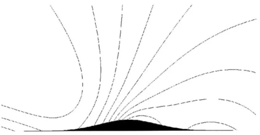
3-1 Adjoint behavior: dual-consistent boundary treatment using only ub(u ). Inviscid Euler flow over Gaussian bump, Moo = 0.5. . . . . 63 3-2 Adjoint behavior: dual-inconsistent boundary treatment using both

u+ and u(u ). Inviscid Euler flow over Gaussian bump, M.. = 0.5. 63 3-3 Adjoint behavior: conservative but dual-inconsistent boundary

treat-ment based on numerical flux function. Inviscid Euler flow over

Gaus-sian bum p, M ,o = 0.5. . . . . 63

3-4 Output convergence: dual-consistent boundary treatment using only ub(uI). Inviscid Euler flow over Gaussian bump, Mo = 0.5. . . . . . 65

3-5 Output convergence: dual-inconsistent boundary treatment using both u+ and ub(u+). Inviscid Euler flow over Gaussian bump, M.. = 0.5.. 66 3-6 Output convergence: conservative but dual-inconsistent boundary

treat-ment based on numerical flux function. Inviscid Euler flow over Gaus-sian bum p, M oo = 0.5. . . . . 66 3-7 Fine NACA 0012 grid, 10752 elements. . . . . 69 3-8 _{Adjoint behavior: dual-consistent treatment with the inclusion of}

in functional. Laminar flow over NACA 0012 airfoil, Moo = 0.5, Re = 5000, a = 2.0 . . . . . 70 3-9 Adjoint behavior: dual-inconsistent treatment without the inclusion of

6b in functional. Laminar flow over NACA 0012 airfoil, Mo = 0.5,

(10)

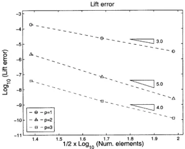
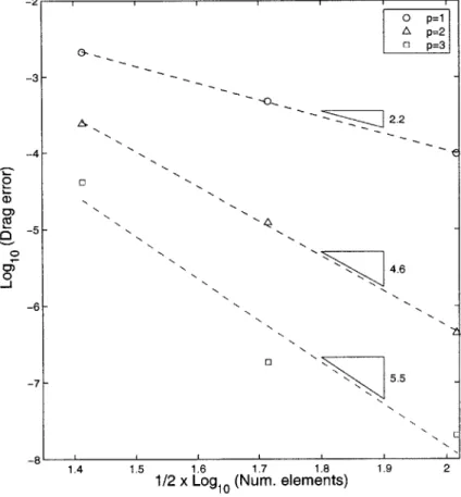
3-10 Drag convergence: dual-consistent treatment with the inclusion of 6b

in functional. Laminar flow over NACA 0012 airfoil, Mo, = 0.5, Re = 5000, a = 2.0 . . . . . 73 3-11 Drag convergence: dual-inconsistent treatment without

o

in

func-tional. Laminar flow over NACA 0012 airfoil, Moo = 0.5, Re = 5000,

a = 2.00 . . . . 74

4-1 Error estimate: dual-consistent boundary treatment using only uh(uj).

Inviscid Euler flow over Gaussian bump, Mo = 0.5. . . . . 87 4-2 Error estimate: dual-inconsistent boundary treatment using both u+

and ub(uI). Inviscid Euler flow over Gaussian bump, Moo = 0.5.. . 87 4-3 Error estimate: conservative but dual-inconsistent boundary treatment

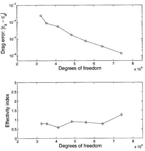
based on numerical flux function. Inviscid Euler flow over Gaussian bum p, M oo = 0.5. . . . . 88 4-4 p-adaptation for drag: output convergence and error estimate. NACA

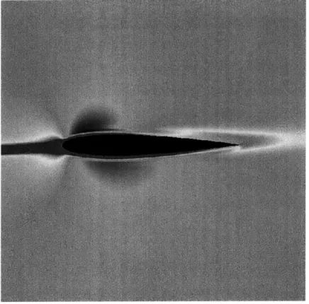
0012 airfoil. Mo = 0.5, Re = 5000, a = 2.0 . . . . . 90 4-5 Contour plots of drag adjoint solution. NACA 0012 airfoil, M"o =

0.5, Re = 5000, a = 2.0 . . . . . 91

4-6 Mach contours. NACA 0012 airfoil, Moo = 0.5, Re = 5000, a = 2.0. 92 4-7 Adapted solution orders: p=1 to p=4. NACA 0012 airfoil, Mo =

0.5, Re = 5000, a = 2.0 . . . . . 93 4-8 p-adaptation for drag using dual-inconsistent treatment: output

con-vergence and error estimate. NACA 0012 airfoil. Moo = 0.5, Re = 5000 , a = 2.0 . . . . 94 4-9 Comparison of adapted solution orders near leading edge, showing p =

4 being utilized for region near the airfoil in the dual-inconsistent case. NACA 0012 airfoil, Mo = 0.5, Re = 5000, a = 2.0 . . . . . 95

5-1 Relative cost of adjoint solution. Inviscid Euler equations. . . . . 107 5-2 Convergence of concurrent flow-adjoint line solver for p = 3

(11)

5-3 Convergence of concurrent flow-adjoint multigrid for p = 3 interpola-tion. Inviscid flow over NACA 0012 airfoil, Mo = 0.5, a= 2.0'. . . . 109 5-4 Convergence of sequential adjoint multigrid for p = 3 interpolation.

Inviscid flow over NACA 0012 airfoil, Mo. = 0.5, a = 2.0 . . . . . 110

5-5 Relative cost of adjoint solution. Compressible Navier-Stokes equations. 112

5-6 Convergence of concurrent flow-adjoint line solver for p = 3

interpo-lation. Laminar flow over NACA 0012 airfoil, Moo = 0.5, Re = 5000,

a = 2.0 . . . . 113 5-7 Convergence of concurrent flow-adjoint multigrid for p = 3

interpola-tion. Laminar flow over NACA 0012 airfoil, Mac = 0.5, Re = 5000,

a = 2.0 . . . . 114

5-8 Convergence of sequential adjoint multigrid for p = 3 interpolation.

Laminar flow over NACA 0012 airfoil, Mo = 0.5, Re = 5000, a = 2.0'. 115

6-1 Samples of Hicks-Henne sine functions for various xm parameters . . . 121 6-2 Full discrete adjoint shape sensitivities (6.2) with respect to

Hicks-Henne sine bump perturbations using p = 5 solution on fine, 9196 element mesh. Gaussian bump, inviscid subsonic flow (Moo = 0.5). . . 122 6-3 Comparison of incomplete and full discrete sensitivities. Gaussian

bump, inviscid subsonic flow (Moo = 0.5) . . . . . 122

6-4 Convergence of incomplete to full discrete sensitivities. Gaussian bump,

inviscid subsonic flow (Moo = 0.5). . . . . 123 6-5 Convergence of Euclidean norm of error in incomplete discrete

sensi-tivities. Gaussian bump, inviscid subsonic flow (Mc = 0.5). . . . . . 124 6-6 Full discrete adjoint shape sensitivities (6.2) on 10752 element fine

mesh using p = 3 solution. NACA 0012, laminar subsonic flow (Mc = 0.5, R e = 5000). . . . . 126 6-7 Comparison of incomplete and full discrete sensitivities for p = 1

(12)

6-8 Comparison of incomplete and full discrete sensitivities for p = 2

solu-tion. NACA 0012, laminar subsonic flow (M.. = 0.5, Re = 5000). . . 128

6-9 Comparison of incomplete and full discrete sensitivities for p = 3

solu-tion. NACA 0012, laminar subsonic flow (Moo = 0.5, Re = 5000). . . 129 6-10 Convergence of incomplete to full discrete sensitivities. NACA 0012,

laminar subsonic flow (Moo = 0.5, Re = 5000). . . . . 130 6-11 Convergence of Euclidean norm of error in incomplete discrete

sensi-tivities for lift output. NACA 0012, laminar subsonic flow (Mo = 0.5,

R e = 5000). . . . . 131

6-12 Convergence of Euclidean norm of error in incomplete discrete sensitiv-ities for drag output. NACA 0012, laminar subsonic flow (Moo = 0.5,

R e = 5000). . . . . 132

7-1 Hicks-Henne sine functions used for airfoil design. . . . . 134

7-2 Results of drag minimization at constant volume. NACA 0012 airfoil,

M oo, = 0.5, Re = 5000, a = 2.0 . . . . . 135

7-3 Results of drag minimization at constant volume. NACA 0012 airfoil,

Moo = 0.5, Re = 5000, a = 2.0 . . . . . 136 7-4 Results of drag minimization at constant volume. NACA 0012 airfoil,

Moe = 0.5, Re = 5000, a = 2.0 . . . . . 137 7-5 Convergence of adaptive precision optimization for drag minimization

at constant volume. NACA 0012 airfoil, M.. = 0.5, Re = 5000, a = 2.0'.138

7-6 Comparison of optimized airfoils computed using fixed p = 1 inter-polation and Adaptive Precision Algorithm for drag minimization at

constant volume. NACA 0012 airfoil, Moo = 0.5, Re = 5000, a = 2.0'. 141

7-7 Results of drag minimization at constant volume and lift. NACA 0012

airfoil, Moo = 0.5, Re = 5000, a = 2.0 . . . . . 145

7-8 Results of drag minimization at constant volume and lift. NACA 0012 airfoil, Moo = 0.5, Re = 5000, a = 2.0 . . . . . 146

(13)

7-9 Results of drag minimization at constant volume and lift. NACA 0012

airfoil, Mo = 0.5, Re = 5000, a = 2.0 . . . . . 147

7-10 Convergence of adaptive precision optimization for drag minimization

at constant volume and lift. NACA 0012 airfoil, Mo = 0.5, Re =

5000 , a = 2.0 . . . . 148

7-11 Comparison of optimized airfoils computed using fixed p = 1

interpo-lation and Adaptive Precision Algorithm for drag minimization at con-stant volume and lift. NACA 0012 airfoil, Moo = 0.5, Re = 5000, a =

2.0 . . . . .. ... . ... ... . .. . . . . . 150 7-12 Mesh for interference inverse design. NACA 0012 airfoils in close

prox-im ity, M o, = 0.5, a = 0.0 . . . . . 152 7-13 Results of interference inverse design. NACA 0012 airfoils in close

proximity, MOo = 0.5, Re = 5000, a = 2.0 . . . . . 154 7-14 Results of interference inverse design. NACA 0012 airfoils in close

proximity, Moo = 0.5, Re = 5000, a = 2.0 . . . . . 155 7-15 Convergence of adaptive precision optimization for interference inverse

design. NACA 0012 airfoils in close proximity, MOo = 0.5, Re =

(14)

(15)

List of Tables

6.1 Euclidean norm of error in incomplete discrete sensitivities. Gaussian

bump, inviscid subsonic flow (M. = 0.5) . . . . 124

6.2 Euclidean norm of error in incomplete discrete sensitivities for lift out-put. NACA 0012, laminar subsonic flow (M. = 0.5, Re = 5000). . . . 131 6.3 Euclidean norm of error in incomplete discrete sensitivities for drag

output. NACA 0012, laminar subsonic flow (M, = 0.5, Re = 5000). . 132

7.1 Computed and exact results for drag minimization at constant volume. NACA 0012, laminar subsonic flow (M, = 0.5, Re = 5000). . . . . . 142

7.2 Computed and exact results for drag minimization at constant volume

(16)

(17)

Chapter 1 Introduction

Aerodynamic design optimization has seen significant development over the past decade. Adjoint-based shape design for elliptic systems was first proposed by Piron-neau [69] and applied to transonic flow by Jameson [49]. A review of the aerodynamic shape optimization literature and a large list of references is given in [46]. Over the years much technology has been developed, allowing engineers to contemplate apply-ing optimization methods to a wide variety of problems. In the context of structured grids, adjoint-based applications include multipoint, multi-objective airfoil design us-ing compressible Navier-Stokes equations [64] and 3D multipoint design of aircraft configurations using inviscid Euler equations [75, 76]. There have also been signif-icant effort in applying adjoint methods to the unstructured grid setting. In this context, Newman et al. [47, 45], Elliot and Peraire [21, 22] were among the first to develop discrete adjoint approaches for the inviscid Euler equations. The work of El-liot and Peraire was also extended to include laminar viscous effects [23]. For 2- and 3D turbulent flows respectively, Anderson and Bonhaus [4], Nielsen and Anderson [66] have developed discrete adjoint implementations for the one-equation turbulence model of Spalart-Allmaras. In [5], Anderson and Venkatakrishnan developed a con-tinuous adjoint approach using unstructured grids. The reverse mode of automatic differentiation has also been applied to both inviscid and Navier-Stokes equations with a two-equation k - e turbulence model [60].

(18)

implemen-tations, there are still obstacles that stand in the way of automatic design methods being widely accepted and applied in the engineering community. In particular, an outstanding issue is the question of reliability of the discrete computational mod-els and its impact on the resulting designs. Lack of trust in the computed results may lead to decreased acceptance and utility of automatic design tools in the engi-neering community, or in an attempt to minimize uncertainty in the computational results, the designer may use unnecessarily refined large-scale models for which the

computational costs quickly become prohibitive.

Currently, the predominant approach towards the optimization of continuous sys-tems is to apply a general nonlinear programming algorithm to discrete models that are at a precision that is fixed prior to optimization. Thus, the chosen algorithm at-tempts to attain the best possible performance for the discrete model but is not aware of the underlying continuous system of interest. An alternative approach described in this thesis is to adaptively control the precision of the discrete model during the optimization. In particular, we propose a method which can ensure that: (1) at each step of the optimization, the objective function for the underlying continuous system is improved; (2) stationary points of the continuous system can be approached to

arbitrary accuracy given enough iterations of the optimization algorithm.

1.1 Objective

The objective of this work is, firstly to develop a framework to increase designer confidence in simulation-based design and, secondly to demonstrate the feasibility of the framework in the context of aerodynamic design.

1.2 Review of related prior work

A major source of model uncertainty arises from the use of coarse discretizations and incomplete solution iteration. To ensure the reliability of the design changes obtained by optimization algorithms based on these approximations, it is necessary

(19)

to accurately estimate the error contributions and effect a mechanism for control. The use of model precision adjustments (or variable fidelity) in optimization has been previously proposed. However, in contrast to our objective these prior efforts were largely driven by the desire to decrease the significant computational effort required to perform optimization, typically for a given high-fidelity model. Below, a review of these work is given in particular examining whether these approaches ensure reliable convergence towards a true optimum for the underlying continuous system, in the sense defined previously.

1.2.1 First-order approximation and model management

The approximation and model management (AMMO) approach proposed by Alexan-drov et al. (see [2] for an overview) is a methodology for utilizing a computationally cheap but low-fidelity model in combination with an expensive, high-fidelity model so that global convergence to a local optimum of the high-fidelity model is guaranteed. In this approach, gradient-based optimization is performed using a low-fidelity model with occasional use of the high-fidelity model to provide a performance measure of the low-fidelity model's predictive quality and recalibrate it via a multiplicative cor-rection. The correction term is constructed so that the low-fidelity model satisfies first-order consistency with the high-fidelity model. Denoting Fo, Fhi to be the objec-tive function obtained from low- and high-fidelity models, the corrected low-fidelity model Fio around the design dk satisfies

Fio(dk) = Fhi(dk), VFlo(dk) = VFhi(dk)-

-A way to enforce the above is to obtain F1 from Fo via a multiplicative correction [2],

(20)

where

#(d)

is a linear function constructed using information from low/high-fidelity models at dk so as to ensure Fi0 satisfies (1.1). This consistency condition is crucial both theoretically for the convergence proof as well as practically in ensuring a good match of trends between the two models. For 2D and 3D wing optimization in inviscid Euler flows and utilizing low/high-fidelity models of same physics but half the mesh spacing, AMMO results in a factor of 2 to 3 compute time saving [2]. When low/high-fidelity models have variable physics as well, the computational saving of AMMO is more significant. The use of AMMO for variable physics models was first demonstrated by Alexandrov et al. [3] and more recently applied by Le Moigne and Qin [62] as well.

AMMO provides a general framework to automatically manage the use of variable fidelity models (of arbitrary accuracies) provided by the user. An inherent assump-tion in AMMO is that the (computable) high-fidelity model is a sufficiently accurate representation of the underlying continuous system. Hence, in the present context where we would like to ensure convergence to the (uncomputable) continuous system, the assumptions made in the AMMO approach are violated. In particular, the gradi-ent information for the continuous system is not available; however, the error in the objective values can usually be estimated. Hence, a different approach based on this assumption is needed.

1.2.2 Progressive optimization

In a series of papers [18, 19, 20], Dadone and Grossman proposed an approach for increasing the efficiency of aerodynamic optimization that relies on converging the analysis and design process simultaneously using progressively finer grids. To decrease the computational costs associated with obtaining the objective function gradient, for inviscid design problems the adjoint state is not solved on the current working grid but on the coarsest grid. For viscous optimization cases, a further approximation is made for the adjoint by ignoring the viscous contribution to the residual. On each given mesh, the flow and adjoint equations are not solved exactly but only converged 1 to 2 orders of magnitude. Once the objective function has decreased

(21)

by an order of magnitude on the current mesh, the mesh spacing is halved and the

same steps are carried out on the new mesh. Among the factors contributing to the efficiency of strategy, it was estimated that the most significant contribution comes from progressively converging the flow solution [19].

The methodology demonstrates significant compute time savings for many aerody-namic design problems. For our purpose of developing a framework that is applicable to general optimization problems for PDE systems, it is not clear that the prescribed strategy is easily extendable without considerable user experience in fine tuning the parameters. In particular, both the desired level of optimization convergence prior to refining the mesh and the drop in the solution residuals in each design cycle may be

highly problem-dependent. We would like to develop an approach that incorporates

a procedure to automatically detect the need to refine mesh or continue iterative solution, in a manner that is generally applicable.

1.2.3 Simultaneous analysis and design

In the simultaneous analysis and design (SAND) or one-shot approach, design updates are not computed from fully converged solutions. Rather, the design and solution ap-proximation are evolved at the same time. Thus, in contast to the reduced variable approach where the primal state is fully determined from the design via the residual equations, for SAND the solution is not required to be feasible until the design ap-proaches optimality. In [54], Kuruvila et al. propose an implementation where the geometry is updated in a hierarchical manner such that high frequency changes are done separately from low frequency changes. Hence, the optimization procedure is broken into a sequence of problems each of its own length scale so as to minimize com-putational costs and improve the conditioning for the optimization problems. The approach is applied to airfoil optimization using the potential flow equations, where the multigrid one-shot strategy is demonstrated to bring the cost of optimization down to two or three times the effort required for one analysis. In [48] the one-shot approach without the use of multiple grids is further applied to inviscid channel and Ringleb flow designs with shape updates obtained via the steepest descent method.

(22)

In [79], interior-point trust-region sequential quadratic programming (SQP) is ap-plied to drag constrained 2D airfoil design in Euler flow. More recently, Sung and Kwon extends approach of [48] to more complex and challenging 2/3D design cases [82, 81]. In the context of optimal control of incompressible Navier-Stokes flows, Ghattas and Bark applied the one-shot strategy using a quasi-Newton approximation for the equations governing the control updates [27]. To improve convergence rate, Biros and Ghattas [14] proposed the use of Krylov method to solve the Newton sys-tem for the Karusch-Kuhn-Tucker (KKT) condition, preconditioned by quasi-Newton SQP with inexact forward and adjoint solves.

Although significant progress has been made, there are a number of issues that remain to be addressed for the SAND approaches. Firstly, it has been observed that these approaches tend to suffer more convergence difficulties in comparison to the traditional reduced-gradient approach [79, 27], motivating Biros et al. to develop globalizing strategies [14]. Also, owing to the lack of theoretical criterion to deter-mine the adequate amount of solution convergence carried out in each design step, numerical experience is needed to find the appropriate trade-off between convergence robustness and efficiency [82]. In addition to convergence instability, another po-tential drawback to SAND approaches is the uncertainty associated with incomplete solution convergence introduced into the design procedure. For instance, in [82] Sung and Kwon described an airfoil optimization test case where the optimized results ob-tained from reduced-gradient and one-shot algorithms are dissimilar. This could be a manifestation of invalid optimization steps in the sense of leading to an increased objective function that allowed the design to escape the basin of attraction and con-verge instead to a neighboring local optimum. While in this case the design concon-verged to another acceptable solution, in other cases this effect could lead to detrimentally degraded designs. A procedure of balancing the degree of feasibility and optimality in the design path to result in added robustness of the algorithm is clearly desirable. Another issue that remains to be addressed is the incorporation of discretization levels into SAND approaches. Most of the SAND strategies are implemented on a single, fine grid. Although in Kuruvila et al. [54] and Shenoy et al. [79] a sequence of

(23)

refined meshes are used in conjunction with the SAND strategy, the refinement criteria used are purely heuristic. Lacking in the current SAND approaches are automatic mesh refinement procedures based on the approximation properties provided by the current mesh and taking into account both the current level of solution convergence and design optimality.

1.2.4 Adaptive precision

Recently, algorithm models for controlling the degree of discretization fidelity and iterative convergence have been proposed by Pironneau and Polak [70]. These consti-tute extensions of previous work by Polak et al. where only the effect of discretization fidelity was of concern [71, 53, 78]. Based on a priori known convergence properties of the discretization formulation and solution procedure, a number of algorithm models are proposed such that precision parameters are controlled within the optimization process. The framework of quasi-consistent approximations ensures that using any op-timizer which produces sufficient decrease in the objective function away from points of zero gradient, every accumulation point of the sequence of iterates constructed

by the algorithm is a stationary point for the underlying continuous system. The

approach has been successfully applied to distributed control problems governed by elliptic equations.

For more complex problems, the approach of Pironneau and Polak may not be applicable since the discretization and iterative convergence properties are not known.

A related issue is that although the algorithm would eventually converge to a

sta-tionary point of the continuous model, it does not guarantee that all design updates computed on intermediate models are valid improvements. Thus, upon termination at a finite optimization index the designer is left unsure whether the obtained design constitutes an improvement over the initial or the observed changes in the computed objective values arise from the use of numerical approximations. Hence, for the given goal of increasing reliability, a further extension is necessary.

(24)

1.3 Approach

The approach taken here is to develop a framework to increase designer confidence that is applicable to general contexts, including aerodynamic optimization. In partic-ular, the approach under consideration is that of successive model refinement which is necessary in order to obtain converging approximations to the underlying continuous system. Furthermore, this approach is arguably more applicable to situations where certain solution features (in the primal and dual variables) may develop during the optimization procedure and hence (local) refinements in the model may be necessary. The framework proposed in this thesis replaces the a priori error estimates uti-lized in Pironneau and Polak's work with a posteriori output error estimates. This approach reduces the uncertainty inherent in a priori error estimates while simul-taneously targeting the outputs for which the optimization is focused on. This a

posteriori framework is discussed in Section 1.3.1. The method is then applied to

aerodynamic optimization using higher-order discontinuous Galerkin discretization of the compressible Euler and Navier-Stokes equations. In Section 1.3.2, the poten-tial benefits of higher-order DGFEM in this context are discussed.

1.3.1 A posteriori error estimation and control in

optimiza-tion

As reviewed in Section 1.2, in all the variable-fidelity techniques other than the adap-tive precision method proposed by Pironneau and Polak [70] a fixed set of high and low fidelity models are chosen a priori, often simply constructed for instance by uniform, global mesh refinements. The computed sequence of designs are only guaranteed to converge to an optimal solution of a fixed finite dimensional model rather than to that of the underlying continuous system. Given the lack of feedback on the model accuracy, there exists no automatic precedure for increasing the refinement of the highest-fidelity model when it is in fact not sufficiently refined for the purpose of optimization or alternatively stopping the procedure when the design changes given by the optimizer may no longer improvements for the underlying continous system.

(25)

There is clearly a need for a precision adjustment framework to ensure the informa-tion provided by the optimizainforma-tion procedure (including the history of designs and computed values of the objective) can be relied upon by the designer.

Recent years has seen the development of a posterior error estimators and bounds in the context of computational simulation. Error estimates for functionals allow one to gain confidence in the computed accuracy for outputs of engineering interest and localization of these estimators give one an ability to perform local refinements where necessary [1, 13, 83, 84, 74, 33, 7]. For exact weak solutions of linear coer-cive PDEs, the existence of functional error bounds in fact allows one to certify the result of the simulation [77]. Application of duality-based analysis technique to the iterative solution of algebraic systems also results in output error estimates due to incomplete solution convergence [68, 37, 57]. In the context of optimal control, there has also been recent effort in using duality-based local error indicators to obtain a se-quence of approximating meshes. For drag reduction in incompressible Navier-Stokes flow via Neumann and Dirichlet boundary control, by applying the general approach proposed for functional outputs [13] Becker used the Lagrangian for the discretized control problem computed with the converged primal and dual states to obtain the subsequent mesh via local mesh refinement [11, 12]. Other potential alternatives exist to obtain meshes that approximate the continuous problem. In the context of Neu-mann boundary control for elliptic systems, Liu et al. [56] perform error analysis for the sum of the norms of the state, adjoint and control errors and adapts the mesh to effect control on these quantities [55].

Although the use of error estimates is becoming prevalent in simulations and local error indicators have been applied to construct sequence of approximating meshes in the optimal control context, the quantitative estimate on the magnitude of the uncertainty in the objective function computed with the approximation models has yet to be incorporated within optimization procedures as a basis for controlling the level of model fidelity for reliability. In this thesis, a posterior error estimates are incorporated within the general adaptive precision framework of Pironneau and Polak

(26)

functions containing unknown constants, the accuracy provided by the discretization in relation to optimization steps as well as the accuracy of solution iteration in relation to discretization level can be appropriately controlled so as to significantly increase the reliability of simulation-based design.

Several connections can be made between the proposed and existing approaches. For instance, the proposed approach of sequencing the grids within optimization can be viewed as an adaptive extension of progressive optimization described in Sec-tion 1.2.2 based on rigorous error estimates. Whereas the latter converges the flow solution by a fixed number of iterations, the proposed approach ensures the iterative error reaches an adaptively chosen tolerance. Also, instead of using a predetermined fine grid, the proposed approach successively refines grids via the current error esti-mator when and where necessary.

1.3.2 High-order DGFEM implementation

To demonstrate the practicality of the proposed methodology, the necessary analy-sis and computational tools are developed in the context of discontinuous Galerkin finite element method (DGFEM). DG schemes have recently become popular for convection-dominated flow problems with the potential of resulting in orders of mag-nitude decrease in simulation time compared to traditional low-order finite volume methods. At least for shock-free flows, it has been demonstrated that given a desired error tolerance on outputs of engineering interest, high-order interpolations can ob-tain estimates with orders of magnitude fewer degrees of freedom in comparison to the use of linear interpolation [25, 67]. In the context of optimal control and shape opti-mization, the use of high-order solution could similarly result in significant efficiency benefits.

Although DGFEM has seen significant development as an analysis tool, it has only recently been applied to the context of optimal control [16] and has yet to be demon-strated in an aerodynamic optimization setting. Owing to the variational properties inherent in its formulation, DGFEM is arguably more amenable to duality analysis than finite volume methods and hence more suitable to the setting of optimal

(27)

con-trol and error estimation. To enable the use of these adjoint-based techniques it is important to examine the dual-consistency property of DG schemes. In particular, the form of boundary treatment has significant effects on adjoint regularity and care needs to be taken to ensure that the primal boundary conditions and functionals are formulated in a dual-consistent manner. This variational property of the numeri-cal scheme turns out also to be crucial for duality-based techniques to fully benefit from the use of high-order solution. Implications of dual-consistency demonstrated in this thesis include the convergence rate in certain error measures, as well as po-tentially benefitting both the effectivity of error estimates and the accuracy of shape sensitivities.

Another essential ingredient for the proposed adaptive precision methodology is the ability to efficiently estimate output error due to incomplete solution. The pro-posed approach is based on the development of a concurrent flow-adjoint solver. Al-though the feasibility of iterative error estimation via concurrent primal-dual itera-tions has been shown in a number of settings [68, 37, 57], it remains to demonstrate that this solution approach can be performed in an efficient manner. It turns out that by making use of the DG properties of nearest neighbor stencil as well as the algebraic construction of adjoint preconditioner and residual, the concurrent solver can obtain the adjoint solution at little additional cost over the flow algorithm. To summarize, a unified adjoint approach is developed in the present DGFEM context for all of discretization and iteration error estimation as well as the computation of

shape sensitivities.

1.4 Contributions

The main contributions of this thesis are in two general areas: firstly, a strategy is proposed for the incorporation of a posteriori estimates into optimization for PDE systems; secondly, the feasibility of the proposed strategy is demonstrated via an application to aerodynamic design. In the latter area, DGFEM is demonstrated as an effective way to realize the proposed methodology. Summing up, the advances

(28)

made in this work include:

" Development of an a posteriori error estimation and control framework for adap-tive precision optimization.

* Demonstration of the feasibility of the proposed framework to aerodynamic optimization.

" Development of duality techniques for high-order DG, including:

- Dual-consistent boundary treatment;

- Efficient concurrent flow-adjoint solution algorithm;

- Accurate adjoint-based estimation of geometric design sensitivities.

1.5 Overview of thesis

In Chapter 2 the setting of consistent approximations is introduced and an adaptive precision framework based on a posteriori error estimates is developed. In Chap-ters 3 to 6 the overarching goals are to build the necessary computational tools for adjoint-based methods within the DG context and verify certain assumptions on the finite dimensional approximations made in the adaptive precision framework. In par-ticular, the numerical examples given at the end of each chapter demonstrate the particular capability required for the adaptive precision computation carried out in

Chapter 7. A number of contributions of independent interest are also made in each chapter. In Chapter 3, a dual-consistent boundary treatment for DG is proposed and implications are illustrated. In Chapter 4, error analysis and control for functional outputs is carried out within a general, optimal control framework applicable to DG schemes. This represents the first treatment of output-based error analysis and adap-tation using the second form of Bassi-Rebay (BR2) discretization. Expressions for local error indicators are derived. Due in part to the dual-consistent property of the chosen DG scheme, the error indicators do capture the local error contribution and the output error is effectively controlled via p-adaptation. In Chapter 5, a concurrent

(29)

flow-adjoint solution algorithm is developed to enable adjoint-based estimation of it-eration error. In particular, it is shown that the nearest-neighbor stencil property of BR2 discretization allows for an efficient adjoint solution algorithm. Furthermore, in the case that the full linearization cannot be stored in memory, the concurrent ap-proach is shown to provide an attractive alternative to the sequential adjoint solution approach in regard to the computational cost. In Chapter 6, the use of an incom-plete shape-sensitivity based on discrete adjoint solution is proposed. Instead of fully differentiating the location of all mesh nodes with respect to the design variables, only surface elements are perturbed while the interior mesh motion is ignored. It is demonstrated that accurate gradient approximations can be obtained from high-order interpolations without including interior mesh motions. To verify the gradient con-vergence assumption made in the adaptive precision framework, the concon-vergence rate of the incomplete to full discrete adjoint sensitivities is studied for various solution orders. In Chapter 7 computational results of applying the adaptive precision frame-work to aerodynamic design cases are presented. Finally, conclusions and potential areas of future work are discussed in Chapter 8.

(30)

(31)

Chapter 2 Adaptive precision methodology

2.1 Introduction

This chapter is concerned with the development of an adaptive precision methodology based on the error estimates that will be developed in the subsequent chapters. Given the underlying concern for reliability and correctness, the main issues addressed here are conditions on the precision adjustments so that design changes computed on the approximation models are valid improvements as well as ensuring the convergence of a sequence of discrete solutions to local optima of the underlying continuous problem. The latter issue of convergence has been examined by Polak et al. in the context of computational optimal control of differential equations via discretized approximations [53, 78, 71] and has more recently been extended to include the use of iterative methods to solve the discrete approximations [70]. This general setting is introduced in Section 2.2. However, the issue of reliability in the algorithm is not addressed by the use of a priori bound functions with its unknown, multiplicative constants that have to be properly tuned in an implementation of the algorithm. The approach to improve the reliability proposed here is to incorporate a posteriori error estimates and is discussed in Section 2.3. By an appropriate choice of parameters in the algorithm, optimization steps on the approximation models are required to satisfy a descent condition for the underlying continuous problem.

(32)

2.2 Consistent approximations

Consider the optimization problem P of minimizing an objective function J(.) over a normed space (D, ||

-

|ID):

(P) : mindED 5(d). (21)

For finite dimensional implementations, consider Dh a sequence of dense finite di-mensional subspaces of D and Ph a sequence of optimization problems for Jh(-):

(Ph)

: mindh EDh Jh(dh)-

(2.2)

The above setting includes the situation where an optimization problem on a PDE model with an infinite dimensional control space is approximated by a sequence of op-timization problems consisting of increasingly finer discretizations over control spaces of expanding dimension. The problems Ph are assumed to provide approximations to P, mathematically described as the convergence of the epigraphs of Ph to that of

P as defined by Polak [71]:

Definition 1 The problems epi-converge (Ph P) if:

-1. For every d

E

D,

3dh

E Dh such that dh -* d and limsup Jh(dh) < (d);

2. For every sequence dh E Dh, dh -+ d E D, liminf jh(dh) ; 5(d).

Although epi-convergence ensures that global optimal solutions of Ph converge to that

of P, it does not ensure that local optima of Ph converge to stationary points of P. As

shown in [71], this may happen if the radius of attraction of the local minimizer for Ph is not bounded away from zero. This is due to the fact that epi-convergence prescribes only zeroth-order characterization of the approximation problems. To preclude this situation, optimality functions Oh(-), 0(.) are introduced to characterize the first-order

(gradient) convergence of the approximations.

Definition 2 Oh(-), 6(-) are optimality functions for Ph, P if they are upper

(33)

respectively.

For the case of continuously differentiable objectives, an example of optimality func-tion is some chosen norm of the gradient. The consistent approximafunc-tion qualificafunc-tion given below on the problem-optimality function pair {P, 6(.)} provides a sufficient condition for the local minima of the finite dimensional approximations to converge to stationary points for the original problem.

Definition 3 The pair {Ph,Oh(-)} form consistent approximations to {P,6(.)} if Ph + P and for every sequence dh E Dh such that dh - d E D, limsupOh(dh) <

8(d).

In particular, the above is satisfied if it can be shown that:

lim dh -+ d - lim Oh(dh) -+ 0(d). (2.3)

h-+0 h-+0

The above condition has been shown in a number of simple settings. For an in-verse design problem on an elliptic PDE via Neumann boundary control, it has been shown that both the objective and optimality function are continuous with respect to boundary control in L2 [61]. By discretizing the continuous system using standard

conforming finite element method (FEM), the sequence of finite-dimensional problems obtained as the mesh diameter goes to zero are consistent approximations in the sense of Definition 3. In the setting of shape optimization, for an inverse design problem of nozzle flow modelled by Laplace's equation with homogeneous Neumann boundary condition enforced on the design surface, it has been shown that both the objective and the optimality function are continuous with respect to shape perturbations in H02. Using standard conforming FEM to approximate the continuous problem, in the limit h -+ 0 both the discrete objective and the optimality functions converge to the corresponding continuous functions as well.

In order to obtain an approximating sequence to some stationary point of problem P via nonlinear programming iterations on the finite-dimensional problems Ph, it is necessary to dynamically adjust the precision parameter h at certain points of the

(34)

computation. In [71], algorithm models are proposed where refinements are based on tests involving either the comparison of optimality function or function changes pro-duced by the underlying nonlinear programming algorithm, with bound functions on the precision of the model Ph. In [70], the algorithm models are further extended to handle the situation where a significant number N of solver iterations are necessary to obtain approximation to the functional output. To decrease the computational time required for optimal control, N is dynamically set with respect to h in a manner so as to ensure convergence. In the situation involving both discretization and iteration parameters, the following assumptions are made on the behavior of the discretization and iteration error [70]. Consider optimization problems where the objective function is a functional of the state u(dh). Let uh(dh) denote a finite dimensional approxima-tion of the state. Also, let uh,N(dh) denote an approximation to Uh(dh) obtained by

N steps of iterative solution.

Assumption 1 For every bounded set B E D, there exists hmax E R+, k < oo, A :R+ -* R+ such that Vh E (0, hmax], dh E Dh

n

B:

IJh(uh(dh), dh) - J(u(dh), dh)j kA(h), (2.4)

and for N E N there exists p : R+ x N --+ R+:

|Jh(Uh,N(dh), dh) - Jh (uh(dh), dh) kp(h, N), (2.5)

where the discretization and iterative bound functions A(.), (-,-) are naturally as-sumed to satisfy the limiting properties,

lim A(h) = 0, h-+O lim p(h, N) = 0, N-oo 3N*(h) lim p(h, N*(h)) = 0. (2.6) h-0

For a given h, equation (2.4) assumes the existence of a bound function kA(h) that holds uniformly on the set Dh

n

B with k being a constant that absorbs the

(35)

depen-dence of the bound on the size of the bounded set B. To prove convergence results, the underlying nonlinear programming algorithm is required to satisfy a monotone, uni-form descent condition [70]. The gradient-based nonlinear programming algorithm

is denoted by the map of controls d' -+ C(di, A'hN) Uh,N, where the gradient is

computed using an adjoint approximation, ?Ph,N, as discussed in Chapter 6.

Assumption 2 For every d* where dJ(d*) _dd

#

0, 3p*, &*, h* > 0, N**(.) < oo such that

Vh < h*, N > N**(h),

Jh(Uh,N(C(dh)), C(dh)) - Jh(uh,N(dh), dh) : ~5*,

Vdh

E

Dh

n

B(d*,

**p*).**

(2.7)

The above condition stipulates that around every non-stationary point d* E D, there exists some ball B of radius p* such that applying the nonlinear programming al-gorithm on all dh E Dh

n

B using gradient information obtained from primal and dual approximations with sufficiently fine h, N would produce an improvement in the computed objective function that is bounded away from zero. With the conditions set out in Assumption 1, the Algorithm Model 2 of [70] based on a nonlinear pro-gramming algorithm satisfying Assumption 2 has the property that if the constructed sequence has any accumulation point then the discretization parameter has to tend zero (h -- 0). Furthermore, every accumulation point of the constructed sequence are

stationary points for

{P, (-)}.

Hence, if

J(-)

is strictly convex with bounded level sets, the algorithm converges to the unique optimum.

2.3 Algorithm based on error estimates

In this work, the bound functions are determined by a posteriori estimates rather than chosen a priori by the user. The former is preferred since the latter is often difficult to realize in many practical situations. An instance of this is the case where the mesh is updated by local p-refinements rather than global h-refinements where both the order of convergence and the required number of solver iterations are difficult to estimate a

(36)

for a particular given dh rather than over some bounded neighborhood. However, if the discretization error for the underlying problem has a smooth dependence on the design with respect to the norm || - ||D, within some small enough set A(h) can be approximated by an a posteriori estimate at the given single design point or obtained by interpolation at a certain set of neighboring design points. Similarly, if for each given discretization the iteration error is assumed to have a smooth dependence on the design then p(h, N) of (2.5) can be obtained via an iteration error estimate for the given design dh.

In the current work, the discretization bound function is simply set to the value of the discretization error estimate computed from partially converged primal and dual state approximations so that A = A(uh,N, 2Ph,N). The specific form of the estimate will be discussed in Chapter 4. Similarly, the iterative bound function is simply set to the value of the iteration error estimate computed from primal and dual state approx-imations, P = O(Uh,N, 4-h,N). The procedure for obtaining Sp(uh,N, bh,N) is discussed in Chapter 5. Also necessary in the algorithm is a function N*(-) satisfying (2.6). Given that asymptotically, limN-+oo A(Uh,N, Ph, N) A(Uh, "Ph) and since A(uh, Ph) vanishes in the limit as h -- 0, a choice for N* (-) satisfying the condition (2.6) is to take it to be the smallest N such that the iterative error is less than a certain (

multiple of A(Uh,N, Oh,N)

N*(h) -- arg min

{I(uh,N,

1h,N) ( X A (uh,N, h,N)}

N

The above choice of N*(h) has the property that a correspondence is maintained between the tolerance level of iterative to discretization error. Using these ingredients, the proposed adaptive precision algorithm taking parameters within the range -Y, ( >

0, r, E E (0, 1), w E (0, 1],

jmax

Z+ is shown below. Adaptive Precision Algorithm (-y, (, T, w, E, jmax)

Initial control: dh E Dh.

Initial converged solution:

(37)

Begin Outer Loop( i:= 0; i < im x)

e Set A := A(uh,N, Oh,N)'

While Inner Loop(

j

:= 0;

j

< jmax)

1. While Line-search

- Compute control update

dh C(dh, Uh,N,

7?Ph,N)-- Concurrently iterate state updates fih,N(dh), g Ndh) until:

(p(flh,N, h,N) T-j X A(1dh,N,'Ph

N)-End Line-search

2. Set p := p(Uh,N

Ph,N)-3. If Jh(Uh,N, dh) - Jh(Uh,N, dh) < -- Exit Inner Loop.

Else

- j := j + 1.

- Concurrently iterate uh,N(dh), Oh,N(dh) until:

(uh,N yh,N <_ (T X A (uh,N i Oh,N -End Inner Loop

e Set

(2.8)

(2.9)

(2.10)

(38)

0

If

Jh(Uh,N, dh) - Jh(Uh,N, dh) >

-- ya(h,

N)W

(2.11)

-

Call

AdaptGrid(E,

dh, Uh,N, 'h,N)'

Else

- Update valid control and states:

{dh;

Uh,N; 4h,N {h; uh,N; 4'h,N

(2.12)

End Outer Loop

The algorithm controls the error in the objective function in a two-tiered manner. In the inner loop, at the trial update dh the iterative error is initially made to be less than a ( multiple of the discretization error term A' at the current design point dh- If

the change in the approximate objective function is not sufficiently negative, as may happen if the approximate gradient does not result in a descent direction, additional solution iterations are performed to tighten the value of iterative error by the factor T. If the iterative error test is satisfied, the computed change in the objective function is tested against -y multiple of the sum of discretization and iteration error contribu-tions,

A(h,

N)w. If the change is not sufficiently negative, the procedure denoted by

AdaptGrid(E, dh, Uh,N, 'h,N) refines the grid according to the local error indicator (as

discussed in Chapter 4) to reduce the error bound in the objective function by the fraction E.

Given parameters in the valid range as described, if the algorithm produces an infinite sequence of iterates d" that has at least one accumulation point, the model precision as governed by h, N can be proved to increase indefinitely. An additional criterion is needed to obtain convergence statements for subsequences of {d'}. A sufficient condition for every accumulation point d* of the constructed sequence {di} to be stationary points for problem P is that for all large enough i, the change in the

(39)

"exact" objective function evaluated with {d'} is negative (Theorem 5, [70]):

J(u(di),d

-

J(u(d

), d)

<

0. (2.13)

In the Algorithm Model 2 presented in [70], w is chosen to be strictly less than 1. In this case, for all choice of precision parameters -y, (, the condition (2.13) would eventually be satisfied for sufficiently large i. In the case that the constant k of (2.4,

2.5) can be estimated effectively, the choice w = 1 can also be made to satisfy the improvement condition (2.13) provided -y is chosen appropriately. In view of the test (2.11) as well as error bounds (2.4) and (2.5), the change in the objective function given by iterates produced by the adaptive precision algorithm is bounded by,

J(u(d+1),d+1) - J(u(d'),d') --

yz

,(h,N) + 2ka(h,N)

=

L

(hN)(--y+2k), (2.14)

which is negative provided -y 2k. Therefore, in the case that the a posteriori error

estimate is tight (k ~ 1) for some appropriate range of designs, setting -y 2 would ensure the inequality (2.13) which has the interpretation that the design updates are always valid in the sense of leading to improvements for the underlying problem P. Given the goal of providing the user confidence in the design updates, the parameter values w = 1, -y = 2 is adopted in this thesis. For the algorithm to be stable and

efficient, the value of the iterative precision parameter ( should also be appropriately chosen. Since the discretization error is estimated using partially converged primal and dual states, a natural requirement is that the iterative error contribution should at least be small in comparison. However, for reasons of efficiency, it should not be chosen unnecessarily small. For computational results shown in Chapter 7,

C

= 0.2 is chosen.

(40)

(41)

Chapter 3 Dual-consistent discretization

In this chapter, the dual-consistency of DGFEM discretizations are discussed. In Section 3.1, the concept of consistency is defined. Past work related to consistency for FEM are discussed in Section 3.2. In Sections 3.3 and 3.4, the dual-consistency of DGFEM discretizations of first- and second-order equations is analyzed. Finally, Section 3.5 demonstrates some of the implications of dual-consistency via application to the Euler and Navier-Stokes equations.

3.1 Dual-consistency

Let V and W be appropriate function spaces. Let u E V be a weak solution to a partial differential equation (PDE) together with a certain set of boundary conditions

(BCs), satisfying

F(u) = 0, (3.1)

where F is an operator mapping V -+ W', with W' being the dual space of W. Let

J(-)

V -+ IR be the functional of interest. Introduce the Lagrangian L : V x W -+ R,

An a posteriori error control framework for adaptive precision optimization using discontinuous Galerkin finite element method