HAL Id: hal-00371757
https://hal.archives-ouvertes.fr/hal-00371757v4
Submitted on 23 Apr 2013
HAL is a multi-disciplinary open access
archive for the deposit and dissemination of
sci-entific research documents, whether they are
pub-lished or not. The documents may come from
teaching and research institutions in France or
L’archive ouverte pluridisciplinaire HAL, est
destinée au dépôt et à la diffusion de documents
scientifiques de niveau recherche, publiés ou non,
émanant des établissements d’enseignement et de
recherche français ou étrangers, des laboratoires
Conditional extremes from heavy-tailed distributions:
An application to the estimation of extreme rainfall
return levels
Laurent Gardes, Stephane Girard
To cite this version:
Laurent Gardes, Stephane Girard. Conditional extremes from heavy-tailed distributions: An
applica-tion to the estimaapplica-tion of extreme rainfall return levels. Extremes, Springer Verlag (Germany), 2010,
13 (2), pp.177-204. �10.1007/s10687-010-0100-z�. �hal-00371757v4�
CONDITIONAL EXTREMES FROM HEAVY-TAILED DISTRIBUTIONS: AN APPLICATION TO THE ESTIMATION
OF EXTREME RAINFALL RETURN LEVELS Laurent Gardes and St´ephane Girard⋆
Team Mistis, INRIA Rhˆone-Alpes & Laboratoire Jean Kuntzmann 655, avenue de l’Europe, Montbonnot, 38334 Saint-Ismier Cedex, France.
⋆ Corresponding author, Stephane.Girard@inrialpes.fr
Abstract− This paper is dedicated to the estimation of extreme quantiles and the tail index from heavy-tailed distributions when a covariate is recorded si-multaneously with the quantity of interest. A nearest neighbor approach is used to construct our estimators. Their asymptotic normality is established under mild regularity conditions and their finite sample properties are illustrated on a simulation study. An application to the estimation of pointwise return levels of extreme rainfalls in the C´evennes-Vivarais region is provided.
Keywords− Conditional extreme quantiles, heavy-tailed distribution, nearest neighbor estimator, extreme rainfalls.
AMS Subject classifications − 62G32, 62G05, 62E20.
1
Introduction
An important literature is dedicated to the estimation of extreme quantiles, i.e. quantiles of order 1 − α with α tending to zero as the sample size in-creases. The most popular estimator was proposed in (Weissman 1978), in the context of heavy-tailed distributions, and adapted to Weibull-tail distributions in (Diebolt et al. 2008; Gardes and Girard 2005). We also refer to (Dekkers and de Haan 1989) for the general case.
When some covariate x is recorded simultaneously with the quantity of in-terest Y , the extreme quantile thus depends on the covariate and is referred in the sequel to as the conditional extreme quantile. In our real data study, we are interested in the estimation of return levels associated to extreme rainfalls as a function of the geographical location. In this case, x is a three-dimensional covariate involving the longitude, latitude and altitude.
Parametric models for conditional extremes are proposed in (Davison and Smith 1990; Smith 1989) whereas semi-parametric methods are considered in (Beirlant and Goegebeur 2003, Hall and Tajvidi 2000). Fully non-parametric estimators have been first introduced in (Davison and Ramesh 2000), where a local polynomial modeling of the extreme observations is used. Similarly, spline
estimators are fitted in (Chavez-Demoulin and Davison 2005) through a penal-ized maximum likelihood method. In both cases, the authors focus on univariate covariates and on the finite sample properties of the estimators. These results are extended in (Beirlant and Goegebeur 2004) where local polynomial estima-tors are proposed for multidimensional covariates and where their asymptotic properties are established.
We propose here to estimate the conditional extreme quantile by a near-est neighbor approach. We refer to (Loftsgaarden and Quesenberry 1965) for the first asymptotic properties of the nearest neighbor density estimator and to (Stone 1977) for the regression case. As an illustration, in the above mentioned climatology study, the estimation of the return level at a given geographical point is based on rainfalls measured at the nearest raingauges. Once the selec-tion of the nearest observaselec-tions is achieved, extreme-value methods are used to estimate the conditional quantile. Whereas no parametric assumption is made on the covariate x, we assume that the conditional distribution of Y given x is heavy-tailed. This semi-parametric assumption amounts to supposing that the conditional survival function decreases at a polynomial rate. The condi-tional tail index γ(x) drives this rate of convergence and has to be estimated before conditional extreme quantiles. In our real data study, the estimation of γ(x) permits to assess the tail-heaviness of the rainfall distribution at each geo-graphical point x, indicating which areas are more likely to suffer from extreme climate events.
Nearest neighbor estimators of the conditional tail-index and conditional extreme quantiles are defined in Section 2. Their asymptotic distributions are derived in Section 3 and some examples are provided in Section 4. The finite sample properties of the estimators on dependent data are illustrated in Sec-tion 5 and an applicaSec-tion to the extreme rainfall study is presented in SecSec-tion 6. Proofs are postponed to Section 7.
2
Nearest neighbor estimators
Let E be a metric space associated to a metric d. For y > 0 and x ∈ E, denote by F (y, x) the conditional distribution function of Y given x. For instance, in the case where E is finite dimensional, each coordinate of x may represent a geographical coordinate. At the opposite, when x is a time series or a curve, E is infinite dimensional. We assume that for all x ∈ E, the conditional distri-bution function of Y is heavy-tailed, see also Gardes and Girard (2008). More specifically, we have for all y > 0,
1 − F (y, x) = y−1/γ(x)L(y, x), (1) or equivalently, for all α ∈ (0, 1],
q(α, x)def= F←(1 − α, x) = α−γ(x)ℓ(α−1, x),
where F←(1 − α, x) = sup{y > 0, F (y, x) ≤ 1 − α} denotes the generalized
inverse of F (., x). Here, γ(.) is an unknown positive function of the covariate x referred to as the conditional tail index. The larger γ(x) is, the heavier is the tail at point x. Besides, for all x ∈ E fixed, L(., x) and ℓ(., x) are slowly varying
functions, i.e. for all v > 0, lim
y→∞
L(vy, x)
L(y, x) = limy→∞
ℓ(vy, x)
ℓ(y, x) = 1. (2)
Let (Y1, x1), . . . , (Yn, xn) be a sample of independent observations from (1). For
a given t ∈ E, our aim is to build an estimator of γ(t) and, for a sequence (αn,t) tending to 0 as n goes to infinity, an estimator of q(αn,t, t). In the sequel,
q(αn,t, .) is referred to as a conditional extreme quantile and we focus on the case
where the design points x1, . . . , xn are non random. Let (mn,t) be a sequence
of integers such that 1 < mn,t < n and let {x∗1, . . . , x∗mn,t} be the mn,t nearest
covariates of t (with respect to the distance d). The associated observations taken from {Y1, . . . , Yn} are denoted by {Z1, . . . , Zmn,t}. The corresponding
order statistics are denoted Z1,mn,t ≤ . . . ≤ Zmn,t,mn,t and the rescaled
log-spacings are defined for all i = 1, . . . , mn,t− 1 as:
Ci,n,t def
= i(log Zmn,t−i+1,mn,t− log Zmn,t−i,mn,t).
Our estimators of γ(t) are linear combinations of these rescaled log-spacings: ˆ γn(t, a, λ) = kn,t X i=1 p (i/kn,t, a, λ) Ci,n,t ,kn,t X i=1 p (i/kn,t, a, λ) , (3)
where (kn,t) is a sequence of integers such that 1 < kn,t < mn,t and the weights
are defined for all s ∈ (0, 1), a ≥ 1, 0 < λ ≤ 1 by p(s, a, λ) = λ
−a
Γ(a)s
1/λ−1(− log s)a−1. (4)
Note that p(., a, λ) is the density function on (0, 1) introduced as the log-gamma distribution by (Consul and Jain 1971). Examples of such densities are provided in Section 4 and illustrated on Figure 1. Four main behaviors can be exhibited: (i) p(., 1, 1) is constant, (ii) p(., 1, λ) is increasing for all 0 < λ < 1, (iii) p(., a, 1) is decreasing for all a > 1 and (iv) p(s, a, λ) has an unique mode at s = exp{λ(1− a)/(1−λ)} for a > 1 and 0 < λ < 1. Let us highlight that other weight functions could be considered in (3) provided that Lemma 3 in Subsection 7.1 still holds. In the same spirit as the quantile estimator proposed by (Weissman 1978), the following estimator of q(αn,t, t) can be derived from (3):
ˆ q(αn,t, t) = Zmn,t−kn,t+1,mn,t µ k n,t mn,tαn,t ¶ˆγn(t,a,λ) ,
where (αn,t) is a sequence in (0, 1). The limiting distributions of these estimators
are established in the next section.
3
Asymptotic results
We first give all the conditions and notations required to obtain the asymptotic normality of our estimators. In the sequel, we fix t ∈ E such that γ(t) > 0. (A.1) The slowly varying function ℓ(., t) is normalized.
Assumption (A.1) is equivalent to supposing that, for α ∈ (0, 1), the Karamata representation of q(α, t) can be simplified as:
q(α, t) = c(t) exp ( Z 1/α 1 γ(t) + ∆(v, t) v dv ) , (5)
with c(t) > 0 and where ∆(v, t) converges to 0 as v goes to infinity. Note also that condition (A.1) implies (1), see for instance (Bingham et al. 1987; Geluk and de Haan 1987). The next two assumptions control the rate of convergence of the function ∆(., t) to zero.
(A.2) The function ∆(., t) is regularly varying with index ρ(t) < 0, i.e. for all v > 0, ∆(vy, t)/∆(y, t) → vρ(t) as y → ∞.
Conditions (A.1) and (A.2) imply that for all v > 0, logµ ℓ(vy, t) ℓ(y, t) ¶ = ∆(y, t) 1 ρ(t)(v ρ(t)− 1)(1 + o(1)),
which is the so-called second-order condition classically used to establish the asymptotic normality of tail-index estimators. The second-order parameter ρ(t) controls the rate of convergence of ∆(v, t) to 0 i.e. the rate of convergence of ℓ(vy, t)/ℓ(y, t) to 1 in equation (2). If ρ(t) is close to 0, this convergence is slow and thus the estimation of the conditional tail index and of the conditional extreme quantile are difficult.
(A.3) The function |∆(., t)| is ultimately decreasing.
In the following, we denote by Vn,t the set {t, x∗1, . . . , x∗mn,t} ⊂ E. The largest
oscillation of the log-quantile function with respect to its second variable is defined for all β ∈ (0, 1/2) as
ωn(β) = sup©|log q(α, x) − log q(α, x′)| , α ∈ (β, 1 − β) , (x, x′) ∈ Vn,t2 ª .
We also assume that (kn,t) is an intermediate sequence which is a classical
assumption in extreme value theory.
(B) mn,t/kn,t→ ∞ and kn,t → ∞ as n → ∞.
We are now in position to state our asymptotic normality result for ˆγn(t, a, λ).
Theorem 1. Suppose (A.1)−(A.3), (B) hold. If, moreover, for some δ > 0, k1/2n,t∆(mn,t/kn,t, t) → ξ(t) ∈ R and k2n,tωn(m−(1+δ)n,t ) → 0 (6)
then
k1/2n,t (ˆγn(t, a, λ) − γ(t) − ∆ (mn,t/kn,t, t) AB(a, λ, ρ(t)))
converges in distribution to a N¡0, γ2(t)AV(a, λ)¢ random variable where
AB(a, λ, ρ(t)) = (1 − λρ(t))−a and AV(a, λ) = Γ(2a − 1)
λΓ2(a) (2 − λ) 1−2a.
The first part of condition (6) is standard in the extreme-value theory. It pre-vents the bias of the estimate from being too large compared to the standard-deviation. The second part of the condition is due to our conditional framework. It is dedicated to the control of the variations with respect to the covariate. For instance, if the slowly varying function ℓ does not depend on the covariate, the second part of condition (6) reduces to a regularity condition on the tail-index:
k2n,tlog(mn,t) sup (x,x′)∈V2
n,t
|γ(x) − γ(x′)| → 0 as n → ∞.
The following result establishes that ˆq(αn,t, t) inherits its asymptotic
distribu-tion from ˆγn(t, a, λ).
Theorem 2. Suppose (A.1)−(A.3), (B) and condition (6) hold. If, moreover, mn,tαn,t< kn,t then kn,t1/2 log³ kn,t mn,tαn,t ´ µ logµ ˆq(αn,t, t) q(αn,t, t) ¶ − log µ kn,t mn,tαn,t ¶ ∆µ mn,t kn,t , t ¶ AB(a, λ, ρ(t)) 
converges in distribution to a N¡0, γ2(t)AV(a, λ)¢ random variable.
The asymptotic bias of estimators ˆγn(., a, λ) and ˆq(αn,t, .) are both proportional
to AB(a, λ, ρ(t)) while their asymptotic variances are proportional to AV(a, λ). These quantities can be controlled by an appropriate choice of a and λ, see Section 4 for a discussion on this topic. Concerning the asymptotic variance, the proportionality factor is γ2(t). Hence, the heavier the tail is, the larger
the asymptotic variance is. Moreover, the asymptotic variance can be lower bounded since
AV(a, λ) − 1 = Z 1
0
(p(s, a, λ) − 1)2ds ≥ 0
which entails that AV(a, λ) ≥ 1 for all a ≥ 1 and λ ∈ (0, 1]. It is thus clear that the minimum variance estimator is obtained with the uniform distribution (a = λ = 1). Let us also highlight that AB(a, λ, ρ(t)) is an increasing function of ρ(t). Thus, the closer ρ(t) is to zero, the larger is the asymptotic bias. However, the second-order parameter ρ(t) is unknown in practice making difficult the comparison of asymptotic bias associated to different log-gamma weights. We refer to (Gomes et al. 2003; Gomes et al. 2004) for estimators of the second-order parameter in the unconditional case. To overcome this problem, one can define the mean-squared bias as:
MSB(a, λ) = Z 0
−∞
AB2(a, λ, ρ)dρ = 1 λ(2a − 1).
Note that the mean-squared bias converges to 0 as a tends to infinity. It it thus not possible to define in our family a minimum mean-squared bias estimator.
4
Choice of log-gamma parameters
4.1
Nearest neighbor Hill estimator
As remarked in the previous section, the minimum variance estimator is ob-tained by letting a = λ = 1 in (4). This choice yields
ˆ γH n(t) = ˆγn(t, 1, 1) = 1 kn,t kn,t X i=1 Ci,n,t.
which is an adaptation of the classical Hill estimator (Hill 1975) to our condi-tional framework. In the following, this estimator is referred to as the nearest neighbor Hill estimator. The asymptotic normality of ˆγH
n(t) is a direct
conse-quence of Theorem 1 with MSB(1, 1) = 1 and AV(1, 1) = 1. The associated conditional quantile estimator ˆqH(α
n,t, t) admits the same limiting distribution
as in Theorem 2.
4.2
Nearest neighbor Zipf estimator
The Zipf estimator, initially introduced in the unconditional case (Kratz and Resnick 1996; Schultze and Steinebach 1996), can be adapted to our framework by remarking that, for i = 1, . . . , kn,t, the pairs¡log(mn,t/i), log Zmn,t−i+1,mn,t
¢ are approximately distributed on a line of slope γ(t). Then, a least-squares estimation yields the following estimator of γ(t):
kn,t X i=1 µi,n,tCi,n,t ,kn,t X i=1
µi,n,t, where µi,n,t= log(kn,t!)/kn,t− log(i!)/i.
It can be shown that µi,n,tis asymptotically equivalent to log(kn,t/i), and thus,
the nearest neighbor Zipf estimator is defined as
ˆ γZ n(t) = ˆγn(t, 2, 1) = kn,t X i=1
log(kn,t/i)Ci,n,t
,kn,t
X
i=1
log(kn,t/i) .
Theorem 1 holds for this estimator with MSB(2, 1) = 1/3 and AV(2, 1) = 2. Similarly, Theorem 2 also holds for the conditional quantile estimator ˆqZ
(αn,t, t)
derived from the nearest neighbor Zipf estimator.
4.3
Controlling the asymptotic mean-squared error
Following Theorem 1, the asymptotic mean-squared error of the estimator ˆγn(t, a, λ)
can be defined as AMSE(a, λ) = ∆2µ mn,t kn,t , t ¶ MSB(a, λ) + γ 2(t)AV(a, λ) kn,t ,
One way to choose the log-gamma parameters could be to minimize the asymp-totic mean-squared error. In practice, the function ∆ is unknown and thus the asymptotic mean-squared error cannot be evaluated. To overcome this
problem, it is possible to introduce an upper bound on AMSE(a, λ). Letting π(a, λ) = MSB(a, λ)AV(a, λ), we obtain for all λ ∈ (0, 1] and a ∈ [1, amax],
AMSE(a, λ) = π(a, λ) kn,t ½ ξ2(t) + o(1) AV(a, λ) + γ2(t) MSB(a, λ) ¾ ≤ π(a, λ) kn,t ©ξ 2(t) + o(1) + γ2(t)(2a max− 1)ª .
We thus propose to consider the log-gamma parameters (aπ, λπ) minimizing
π(a, λ), leading to the estimator ˆγπ
n(t, a, λ) = ˆγn(t, aπ, λπ). Annulling the partial
derivative of π(a, λ) with respect to λ yields λπ= 4/(1 + 2aπ) whereas it is not
possible to find an explicit value for aπ. A numerical optimization yields aπ ≈
2.19. Theorem 1 holds with MSB(aπ, λπ) ≈ 0.40 and AV(aπ, λπ) ≈ 1.51, and
Theorem 2 holds for the corresponding conditional quantile estimator ˆqπ(α n,t, t).
4.4
Discussion
The three previously introduced log-gamma densities are represented on Fig-ure 1. The nearest neighbor Hill estimator gives the same weight to all the kn,t largest observations. The nearest neighbor Zipf estimator corresponds to
a decreasing log-gamma density. Finally, the log-gamma density used in ˆγπ n(.)
has a mode in (0, 1). A heavy left tail for the log-gamma distribution (4) gives large weights to large observations in (3) and yields large asymptotic variances:
AV(2, 1) > AV(aπ, λπ) > AV(1, 1).
Asymptotic bias have an opposite behavior:
MSB(2, 1) < MSB(aπ, λπ) < MSB(1, 1).
It is thus not possible to find log-gamma parameters giving rise to the best estimator both in terms of asymptotic bias and variance. However, for a given mean-squared bias, the best asymptotic variance can be computed. Letting MSB(a, λ) = b, we obtain λ(a, b) = 1/(b(2a − 1)) and consequently
AV(a, λ(a, b)) = bΓ(2a) Γ2(a) ½ 2 − 1 b(2a − 1) ¾1−2a ,
where a ≥ max{1, (1 + b)/(2b)} in order to ensure 0 < λ(a, b) ≤ 1. The optimal asymptotic variance for a fixed mean-squared bias b is obtained by minimizing this quantity with respect to a:
OAV(b) = min
a≥max{1,(1+b)/(2b)}AV(a, λ(a, b)).
Here again, an explicit solution is not available. The graph of the function OAV obtained by numerical optimization is depicted on Figure 2. Some level curves of π(a, λ) are also represented. It appears that ˆγπ
n and ˆγnH can be considered
as optimal estimators since, for a fixed value of the mean-squared bias, they have the optimal asymptotic variance. In contrast, the nearest neighbor Zipf estimator is not optimal. It is possible to build an estimator with the same mean-squared bias (= 1/3) and smaller asymptotic variance (≈ 1.85).
5
Simulation study
The asymptotic properties of our estimators are established in Section 3 under an independence assumption. This hypothesis may not be verified on rainfall data where temporal and/or spatial dependence is expected, see Section 6. The impact of temporal and spatial dependence on the bias and variance of the tail-index estimator ˆγπ
n is illustrated in Subsection 5.1 and 5.2 respectively.
5.1
Temporal dependence
Here, for the sake of simplicity, we do not introduce a covariate information, the conditional estimator being studied in the next paragraph. A temporal series {y1, . . . , yn} with n = 500 is generated following the method proposed by
(Fawcett and Walshaw 2007): First, a temporal series {f1, . . . , fn} with standard
Fr´echet margins is simulated. The joint distribution of (fi, fi+1), i = 1, . . . , n−1
is given by a bivariate extreme-values distribution G(u, v) = exp{−V (u, v)} with a logistic dependence function V (u, v) = (u−1/α+ v−1/α)α, u > 0, v > 0
and α ∈ (0, 1]. Note that α tunes the dependence between two consecutive observations: α = 1 leads to the independent case while α → 0 corresponds to complete dependence. The following procedure is used:
1. Simulate the first observation f1from the standard Fr´echet distribution.
2. For i = 1, . . . , n − 1: Compute the conditional distribution of fi+1 given
fi and simulate fi+1 from this distribution.
Finally, the temporal series {f1, . . . , fn} is transformed so that the margins are
Burr distributed. Recall that the Burr distribution function is given for y ≥ 0 by 1 − (1 + y−ρ/γ)1/ρ where ρ is the second order parameter as defined in condition
(A.2). Here, we set ρ = −1 and γ = 0.2. Using this strategy, N = 100 temporal series with Burr margins are simulated. The estimator ˆγπ
n is computed on each
replication, leading to N values {ˆγπ
n,1, . . . , ˆγn,Nπ }, with ˆ γn,jπ = k X i=1 pµ i k, aπ, λπ ¶ i logà y (j) n−i+1,n y(j)n−i,n ! , k X i=1 pµ i k, aπ, λπ ¶ , where y1,n(j) ≤ . . . ≤ y (j)
n,n is the j−th temporal series ranked in ascending order.
The empirical squared bias (ESB) and the empirical variance (EV) defined by
ESB = 1 N N X j=1 (ˆγn,jπ − γ)2and EV = 1 N N X j=1 ˆγπn,j− 1 N N X j=1 ˆ γπn,j 2
are represented on Figures 3 and 4 as functions of the sample fraction k and for different values of the dependence coefficient α ∈ {1, 0.8, 0.5, 0.2}. It appears on Figure 3 that, even for a strong dependence (α = 0.2), a good choice of k leads to an estimator with small bias. Thus, focusing on the bias, the main problem in estimating the tail index with temporally dependent observations is more on the choice of the sample fraction than on the dependence degree. Turning to the variance of ˆγπ
n, Figure 4 shows that it increases with the temporal dependence
degree. Note that these remarks are consistent with the conclusions drawn in (Fawcett and Walshaw 2007).
5.2
Spatial dependence
This paragraph is dedicated to the illustration of spatial dependence conse-quences on the conditional tail index estimation. Using Subsection 5.1 strategy, ns = 10 independent temporal series {s1, . . . , sns} of size 500 with standard
normal margins are simulated. The temporal dependence coefficient is fixed to α = 0.5. Here, nscan be interpreted as the number of gauged stations and the
total number of observations is thus n = 5000. Spatial correlation is introduced by defining (s′
1, . . . , s′ns) = (s1, . . . , sns)A(θ) where A(θ) is a ns× ns circulant
matrix defined for all θ ∈ [0, 1] and (i, j) ∈ {1, . . . , ns}2 by:
Ai,j(θ) =
½
1/δ if δ > (j − i) modulo ns,
0 otherwise
with δ = ⌊ns− (ns− 1)θ⌋, ⌊.⌋ denoting the integer part. Parameter θ tunes the
spatial dependence between the temporal series {s′
1, . . . , s′ns}: Each series s
′ j is
the mean of δ temporal series taken in the set {s1, . . . , sns}. For instance, θ = 1
leads to δ = 1, A(1) is the identity matrix and thus s′
1, . . . , s′ns are independent.
At the opposite, θ = 0 yields δ = ns and s′1 = . . . = s′ns which corresponds to
the complete dependence case. An intermediate case is θ = 4/5 which leads to δ = 2 and s′
1= (s1+ s2)/2, s′2= (s2+ s3)/2, . . . when ns= 10.
Finally, each series s′
j, j = 1, . . . , ns is transformed so that its margins
are Burr distributed with second order parameter ρ = −1 and conditional tail index γj = 0.16 + j(0.26 − 0.16)/ns. In order to illustrate the influence of the
spatial dependence on the estimation of the conditional tail index, the empirical mean squared error (defined by EMSE = EV + ESB) is computed on N = 100 independent replications of the ns temporal series for θ ∈ {1, 0.8, 0.5, 0.2} and
m ∈ {500, 500 × 2, . . . , 500 × ns}. Since the effect of the sample fraction k
has been investigated in Subsection 5.1, it is now fixed to the value minimizing the EMSE. Results are represented on Figure 5. It appears that the spatial dependence coefficient θ does not influence much the estimation error. A more detailed study revealed that dependence slightly increases the bias but decreases the variance, leading to small fluctuations of the empirical mean squared error. Besides, it is also apparent that taking account of nearest neighbors permits to reduce the EMSE.
6
Application to rainfall data
Extreme rainfall statistics are often used when a flood occurred to assess the rar-ity of such an event. A typical question is to estimate what is the amount of rain on one hour that is expected to be exceeded once every T years. Mathematically speaking, the problem is to estimate the T -years quantile q(1/(365 × 24T ), .) of the hourly rainfall.
In (Coles and Tawn 1996), a Bayesian approach is used to model extreme precipitations at a location in south-west England. The excess distribution is represented by a Generalized Pareto Distribution (GPD) with some prior information on its parameters. (Cooley et al. 2007) take profit of the Bayesian framework to model GPD parameters with stochastic processes depending on some geographical variables. An alternative approach consists in modeling the rainfall process itself by a max-stable process. We refer to (Buishand et al. 2008;
Padoan et al. 2009) for applications to the daily rainfalls in the Netherlands and in the USA respectively. Here, we consider hourly rainfall observations at 142 stations in the C´evennes-Vivarais region (southern part of France) from 1993 to 2000. In this context, the variable of interest Y is the hourly rainfall and the covariate x is the three dimensional geographical location (x1 is the
longitude, x2 is the latitude and x3 is the altitude). The set of coordinates
S = {(x1,j, x2,j, x3,j), j = 1, . . . , 142} of the raingauge stations is depicted on
Figure 6. The total number of observations is n = 264056. The extreme rainfall in the C´evennes-Vivarais region has already been studied in (Bois et al. 1997). The data consisted in hourly rainfalls measured at 48 raingauge stations from 1948 to 1991. The 10-years quantile is estimated under a Gumbel assumption and using a kriging technique.
Let us first focus on the estimation of the conditional tail index γ(x) as a function of x. To this aim, the three previously described estimators ˆγH
n, ˆγ
Z
n and
ˆ γπ
n are used. All of them depend on the choice of mn,tand kn,t. For the sake of
simplicity, these parameters are chosen to be independent of the location t. They are selected by minimizing some dissimilarity measure between the estimators:
(ˆk, ˆm) = arg min k,m X t∈S D(ˆγH n(t), ˆγ Z n(t), ˆγnπ(t))
with D(u1, u2, u3) = (u1− u2)2+ (u2− u3)2+ (u3− u1)2. This heuristics is
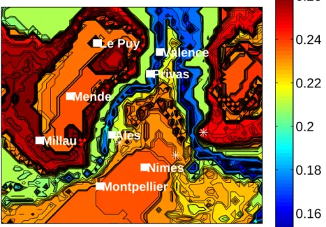
sometimes used in nonparametric estimation. It relies on the idea that, for a properly chosen pair (ˆk, ˆm), all three estimates should approximately give the same tail index. We refer to (Gardes et al. 2010) for an illustration of this procedure on simulated data. It appears that it behaves similarly to an Oracle method which minimizes the distance to the true function γ(t) associated to the simulated data. Here, this procedure yields ˆm/n = 25% and ˆk/ ˆm = 0.1%. Note that the graphical representation of the estimated tail index as a function of a three dimensional covariate is not possible. The role of the altitude x3 is illustrated on Figure 7 while the role of the planar coordinates
(x1, x2) is represented on Figure 8. The shapes of the three curves representing
the estimated tail index as a function of the altitude are qualitatively the same. The estimated tail indices are decreasing functions of the altitude till x3= 400
meters and are increasing for altitudes ranging from 400 and 1600 meters. For the visualization sake, the estimators have been computed on a regular grid over the considered geographical region. This grid is depicted on Figure 6 and involves 60 × 50 ungauged locations. The result are presented on Figure 8 where ˆγπ
n is represented as a function of the longitude and latitude. The large
estimated values (ˆγnπ ∈ [0.15, 0.28]) are consistent with the credibility intervals
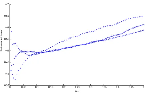
found in (Coles and Tawn, 1996) but contradict the Gumbel assumption of (Bois et al. 1997). To compare both approaches, we focus on three stations: Deaux, Bedoin and Chateauneuf-de-Gadagne (localized from left to right by a ∗ on Figure 8). These three stations measured hourly rainfalls larger than 100 millimeters (mm). For each of the above stations, ˆγπ
n is computed without
using neighbor stations, i.e using a standard pointwise approach. The number of upper order statistics varies for each station such that kn,t/mn,t∈ {0, . . . , 50%}.
Results are presented on Figure 9. It appears that, for all values of kn,t, the
estimated tail indices are larger than 0.35. The Gumbel assumption seems therefore to be unrealistic. Let us note that, when the neighborhood information
is taken into account (Figure 8), the geographical smoothing leads to smaller estimated tail indices, but still larger than 0.15.
Similar results are obtained concerning the 10-years return level. It appears on Figure 10 that the considered return level is globally decreasing with the altitude. However, the observed variability indicates that altitude is not the unique factor. Indeed, one can see on Figure 10 that the Valence area of Rhˆone Valley does not suffer from high pointwise return levels whereas the southern part does.
The drift of the rainfall rate as a function of the altitude is in agreement with the rainfall descriptive statistics in the region (Molini´e et al. 2008). Since in this region low altitude areas are flat areas and are closed to the sea, the deconvolution of physical processes involved in such an altitude-rainfall rate relationship is complex. Therefore, the enhancement of extreme rainfall rates could be either a regional specificity: the supply of warm and moist air by northward low level winds over the Mediterranean sea; or a more universal phenomena: flat areas are the most efficient in capturing the solar energy which is in turn available to involve deep convective clouds.
Unsurprisingly, the estimated return levels are higher than those found in (Bois et al. 1997), ranging from 30mm to 65mm under the Gumbel assumption. In view of our data, these return levels seem under-estimated since 7 over the 142 considered stations measured rainfalls larger than 80mm and 3 of them measured rainfalls larger than 100mm.
Finally, let us emphasize that our results are obtained under both an in-dependence and a temporal stationarity assumption. Following (Fawcett and Walshaw 2007) and our simulation study (Section 5), it seems that temporal and/or spatial dependence has little effect on the estimation bias. However, the influence of dependence on the variance prevents us from directly deriving confidence intervals from the asymptotic results established in Section 3. Con-cerning the temporal stationarity assumption, the short observation period (7 years) does not allow to discern any trend in the time series. However, it would be interesting to take seasonal effects into account. To this end, our further work will consist in splitting the data into homogeneous time periods. Such seasonal approaches have already been considered in Bayesian models (Coles and Pericchi 2003; Coles et al. 2003).
7
Proofs
Some preliminary results are given in Subsection 7.1. Their proofs are postponed to Subsection 7.3 while main results are proved in Subsection 7.2. For the sake of simplicity, in the sequel, we note ktfor kn,t, ∆tfor ∆(mn,t/kn,t, t), αtfor αn,t
and mt for mn,t. Letting Jkt = {1, . . . , kt} and Jmt = {1, . . . , mt}, we finally
introduce
• {Vi, i ∈ Jmt} a set of independent standard uniform variables,
• V1,mt ≤ . . . ≤ Vmt,mt the associated order statistics,
7.1
Preliminary results
The first lemma provides a representation in distribution of the logarithm of the observations whose covariate is in the neighborhood of t.
Lemma 1. Under (A.1) and (A.3), if kt/mt → 0 and kt2ωn(m−(1+δ)t ) → 0
for some δ > 0, then, there exists a sequence of events (An) with P(An) → 1 as
n → ∞ such that { log Zmt−i+1,mt, i ∈ Jkt| An} has the same distribution as
n log q(Vi,mt, t) + OP(ωn(m −(1+δ) t )), i ∈ Jkt ¯ ¯ ¯ An o .
In order to be self-contained, we quote a lemma proved in (Beirlant et al. 2002). This result provides an exponential regression model for rescaled log-spacings. Lemma 2. Suppose (A.1), (A.2) and (B) hold. Then, the random vector {i(log q(Vi,mt, t) − log q(Vi+1,mt, t)), i ∈ Jkt} has the same distribution as
(Ã γ(t) + ∆ µ i kt+ 1 , t ¶−ρ(t)! Fi+ βi,n(t) + oP(∆t) , i ∈ Jkt ) , where Pkt j=1 ³ 1 j Rj/kt 0 u(ν)dν ´
βi,n(t) = oP(∆t), for every function u defined on
(0, 1) satisfying ¯ ¯ ¯ ¯ ¯ kt Z j/kt (j−1)/kt u(ν)dν ¯ ¯ ¯ ¯ ¯ ≤ g µ j kt+ 1 ¶ , (7)
for some fixed positive continuous function g(., t) defined on (0, 1) and satisfying Z 1
0
max(1, log(1/s))g(s)ds < ∞. (8) In the following lemma, an integral representation of log-gamma weights is es-tablished.
Lemma 3. Let a ≥ 1 and 0 < λ ≤ 1. There exists a function u satisfying (7) and (8) such that for all j ∈ Jkt,
p(j/kt, a, λ) = 1 j Z j/kt 0 u(ν)dν.
Finally, the following lemma is a simple unconditioning tool for determining the asymptotic distribution of a random variable. We refer to (Gardes et al. 2010) for a proof.
Lemma 4. Let (Xn) and (Yn) be two sequences of real random variables.
Sup-pose there exists a sequence of events (An) such that (Xn|An) d
= (Yn|An) with
7.2
Proofs of main results
The following result is a consequence of Lemmas 1–3. It establishes a represen-tation of log-spacings in terms of standard exponential random variables which is the cornerstone of the proof of Theorem 1. We refer to (Falk et al. 2004, Theorem 3.5.2) for the approximation of the nearest neighbors distribution us-ing the Hellus-inger distance and to (Gangopadhyay 1995) for the study of their asymptotic distribution.
Proposition 1. Suppose (A.1), (A.2), (A.3) and (B) hold. If, moreover, k2
tωn(m−(1+δ)t ) → 0 for some δ > 0 then
{Ci,n,t, i ∈ Jkt|An} d = {Ci,n,t(1) + Ci,n,t(2) , i ∈ Jkt|An} where {Ci,n,t(1) , i ∈ Jkt} d = (Ã γ(t) + ∆ µ i kt+ 1 , t ¶−ρ(t)! Fi+ βi,n(t) + oP(∆t) , i ∈ Jkt ) Ci,n,t(2) = OP ³ ktωn(m−(1+δ)t ) ´ uniformly in i ∈ Jkt. and with 1 kt kt X i=1 p(i/kt, a, λ)βi,n(t) = oP(∆t). (9)
Proof of Proposition 1− From Lemma 1, {Ci,n,t, i ∈ Jkt|An} d = ½ i log µ q(Vi,mt, t) q(Vi+1,mt, t) ¶ + iOP ³ ωn(m−(1+δ)t ) ´ , i ∈ Jkt|An ¾ = {Ci,n,t(1) + C (2) i,n,t, i ∈ Jkt|An},
where Ci,n,t(1) = i(log q(Vi,mt, t)−log q(Vi+1,mt, t)) and C
(2)
i,n,t= iOP(ωn(m−(1+δ)t )).
From Lemmas 2 and 3, {Ci,n,t(1) , i ∈ Jkt} has the same distribution as
(Ã γ(t) + ∆t µ i kt+ 1 ¶−ρ(t)! Fi+ βi,n(t) + oP(∆t) , i ∈ Jkt ) , with 1 kt Pkt
i=1p(i/kt, a, λ)βi,n(t) = oP(∆t). Finally, for all i ∈ Jkt, we have
Ci,n,t(2) = OP
³
ktωn(m−(1+δ)t )
´
, and the result is proved.
Proof of Theorem 1− Let us consider the random variables defined as Λ(1)n = k 1/2 t {ˆγn(t, a, λ) − γ(t) − ∆tAB(a, λ, ρ(t))} Λ(2)n = k 1/2 t kt X i=1 ˜ p(i/kt, a, λ)(Ci,n,t(1) + C (2) i,n,t) − γ(t) − ∆tAB(a, λ, ρ(t)),
where the following normalized weights ˜p(i/kt, a, λ), i = 1, . . . , kt have been
introduced ˜ p(i/kt, a, λ) = p(i/kt, a, λ) ,kt X j=1 p(j/kt, a, λ) .
Proposition 1 states that {Λ(1)n |An} = {Λd (2)n |An}. From Lemma 4, to prove
Theorem 1, it is sufficient to show that Λ(2)n converges in distribution to a
N (0, γ2(t)AV(a, λ)) random variable. Introducing
T1,n= kt X i=1 p(i/kt, a, λ)(Fi− 1), T2,n= kt X i=1 p(i/kt, a, λ) µ i kt+ 1 ¶−ρ(t) (Fi− 1), T3,n= kt X i=1 p(i/kt, a, λ)βi,n(t), T4,n= ∆t kt X i=1 p(i/kt, a, λ) µ i kt+ 1 ¶−ρ(t) , T5,n= kt X i=1 p(i/kt, a, λ), T6,n= Ãkt X i=1 p2(i/kt, a, λ) !1/2 , Proposition 1 entails the following expansion:
T5,n T6,n Ãkt X i=1 ˜ p(i/kt, a, λ)Ci,n,t(1) − γ(t) − T4,n T5,n ! d = γ(t)T1,n T6,n + ∆t T2,n T6,n +T3,n T6,n + T5,n T6,n oP(∆t). (10)
From Lindeberg theorem, a sufficient condition for T1,n/T6,n d → N (0, 1) is kt X i=1 p3(i/kt, a, λ)/T6,n3 → 0. (11)
Since for any integrable function ϕ, the following convergence of Riemann sum holds, 1 kt kt X i=1 ϕµ i kt ¶ → Z 1 0 ϕ(s)ds (12)
it follows that T6,n= k1/2t AV(a, λ)1/2(1 + o(1)). Thus, using (12), we have
1 kt kt X i=1 p3(i/kt, a, λ) = Γ(3a) Γ3(a)(3 − 2λ) −3a(1 + o(1)), and thereforePkt
i=1p3(i/kt, a, λ)/T6,n3 = O(k −1/2
t ), showing that condition (11)
is satisfied and
T1,n/T6,n d
→ N (0, 1). (13)
Next, let us focus on T2,n/T6,n. Remarking that this term is centered with finite
variance, it follows that
T2,n/T6,n= OP(1). (14)
Equation (9) in Proposition 1 yields
T3,n/T6,n= oP(k1/2t ∆t) = oP(1). (15)
Finally, from (12) we obtain,
T4,n/T5,n = ∆tAB(a, λ, ρ(t))(1 + o(1)), (16)
Replacing (13)–(17) in (10) shows that kt1/2 Ãkt X i=1 ˜
p(i/kt, a, λ)Ci,n,t(1) − γ(t) − ∆tAB(a, λ, ρ(t))
!
converges in distribution to a N (0, γ2(t)AV(a, λ)) random variable. Taking
account of kt1/2 kt X i=1 ˜ p(i/kt, a, λ)Ci,n,t(2) = OP(kt3/2ωn(m−(1+δ)t )) = oP(1)
concludes the proof.
Proof of Theorem 2− Let us consider the following expansion: logµ ˆq(αt, t) q(αt, t) ¶ − log µ kt mtαt ¶ ∆tAB(a, λ, ρ(t)) = logµ Zmt−kt+1,mt q(kt/mt, t) ¶ + {ˆγn(t, a, λ) − γ(t) − ∆tAB(a, λ, ρ(t))} log µ k t mtαt ¶ − ½ log µ q(α t, t) q(kt/mt, t) ¶ − γ(t) log µ k t mtαt ¶¾ = ζ1,n+ ζ2,n+ ζ3,n.
First, from Lemma 1, ζ1,n d
= log q(Vkt,mt, t)−log q(kt/mt, t)+OP(ωn(m
−(1+δ)
t )),
and assumptions (A.1), (A.3) imply that ¯ ¯ ¯ ¯ logµ q(Vkt,mt, t) q(kt/mt, t) ¶¯ ¯ ¯ ¯ = OP(∆t) ¯ ¯ ¯ ¯ logµ mt kt Vkt,mt ¶¯ ¯ ¯ ¯ . Moreover, under (B), it is well-known that kt1/2((mt/kt)Vkt,mt− 1)
d
→ N (0, 1), (see for instance (Girard 2004)) and thus
ζ1,n= OP(∆tkt−1/2) + OP(ωn(m−(1+δ)t )). (18)
Besides, from Theorem 1, we have k1/2t / log(kt/(mtαt))ζ2,n
d
→ N (0, γ2(t)AV(a, λ)), (19)
and, finally, (5) entails that log µ q(α t, t) q(kt/mt, t) ¶ = γ(t) log µ k t mtαt ¶ + Z 1/αt mt/kt ∆(u, t) u du. Since 1/αt> mt/kt, (A.3) yields
|ζ3,n| ≤ Z 1/αt mt/kt |∆(u, t)| u du ≤ ∆tlog µ kt mtαt ¶ (20) and collecting (18)-(20) concludes the proof.
7.3
Proofs of auxiliary results
Proof of Lemma 1− Under (A1) the function q(., t) is continuous. Since the random variables {Zi, i ∈ Jmt} are independent, we have:
{log Zi, i ∈ Jmt}
d
= {log q(Vi, x∗i), i ∈ Jmt},
where x∗
i is the covariate associated to Zi. Denoting by ψ(i) the random index
of the covariate associated to the observation Zmt−i+1,mt, we obtain
{log Zmt−i+1,mt, i ∈ Jmt}
d
= {log q(Vψ(i), x∗ψ(i)), i ∈ Jmt}.
Let us consider the event An = A1,n∩ A2,nwhere
A1,n = ½ min i∈Jkt\{kt} log µ q(Vi,mt, ui) q(Vi+1,mt, ui+1) ¶ > 0, ∀(u1, . . . , ukt) ∈ Vn,t ¾ and A2,n = ½ min i∈Jmt\Jktlog µ q(Vkt,mt, ukt) q(Vi,mt, ui) ¶ > 0, ∀(ukt+1, . . . , umt) ∈ Vn,t ¾ . Conditionally to A1,n, the random variables q(Vi,mt, ui), i ∈ Jkt are ordered as
q(Vkt,mt, ukt) ≤ q(Vkt−1,mt, ukt−1) ≤ · · · ≤ q(V1,mt, u1),
and, conditionally to A2,n, the remaining random variables q(Vi,mt, ui), i ∈
Jmt\ Jkt are smaller since
max
i∈Jmt\Jktq(Vi,mt, ui) ≤ q(Vkt,mt, ukt).
Thus, conditionally to An, the kt largest random values taken from the set
{log q(Vψ(i), x∗ψ(i)), i ∈ Jmt} are {log q(Vi,mt, x
∗ ψ(i)), i ∈ Jkt}. Consequently, letting Ti def = x∗ ψ(i), we have: {log Zmt−i+1,mt, i ∈ Jkt|An} d = {log q(Vi,mt, Ti), i ∈ Jkt|An} .
To conclude the proof, it remains to show that
log q(Vi,mt, Ti) − log q(Vi,mt, t) = OP(ωn(m
−(1+δ)
t )), (21)
uniformly in i ∈ Jkt and that
P(An) → 1, (22)
as n → ∞. Let us consider the event A3,n= {V1,mt > δmt}∩{Vmt,mt< 1−δmt},
where δmt = m
−(1+δ)
t . Under A3,n, we have δmt < Vi,mt < 1 − δmt for all
i ∈ Jmt. Hence,
P ³|log q(Vi,mt, Ti) − log q(Vi,mt, t)| > ωn(m
−(1+δ)
t )
´
≤ P ³|log q(Vi,mt, Ti) − log q(Vi,mt, t)| > ωn(m
−(1+δ) t ) ¯ ¯ ¯ A3,n ´ P(A3,n) + P(AC3,n), where AC
3,n is the complementary event associated to A3,n. Since under A3,n,
|log q(Vi,mt, Ti) − log q(Vi,mt, t)| ≤ ωn(m
−(1+δ)
for all i ∈ Jkt, it is clear that
P³|log q(Vi,mt, Ti) − log q(Vi,mt, t)| > ωn(m
−(1+δ) t ) ¯ ¯ ¯ A3,n ´ = 0. Remarking that P(A3,n) ≥ P(V1,mt > δmt)+P(Vmt,mt < 1−δmt)−1 = 2P(V1,mt > δmt)−1 → 1, since Vmt,mt d = 1 − V1,mt and P(V1,mt > δmt) = (1 − δmt) mt → 1 concludes the
proof of (21). Furthermore, for all (ui, uj) ∈ Vn,t2 , we have, on the one hand
logµ q(Vj,mt, uj) q(Vi,mt, ui) ¶ = logµ q(Vj,mt, t) q(Vi,mt, t) ¶ + logµ q(Vj,mt, uj) q(Vj,mt, t) ¶ + logµ q(Vi,mt, t) q(Vi,mt, ui) ¶ ≥ logµ q(Vj,mt, t) q(Vi,mt, t) ¶ − 2ωn(δmt),
and on the other hand, min i∈Jmt\Jktlog µ q(Vkt,mt, ukt) q(Vi,mt, ui) ¶ ≥ min i∈Jmt\Jktlog µ q(Vkt,mt, t) q(Vi,mt, t) ¶ − 2ωn(δmt) ≥ log µ q(Vkt,mt, t) q(Vkt+1,mt, t) ¶ − 2ωn(δmt).
Consequently, considering the event A4,n= ½ min i∈Jktlog µ q(Vi,mt, t) q(Vi+1,mt, t) ¶ > 2ωn(δmt) ¾ ,
it is clear that A3,n∩ A4,n⊂ An. It thus remains to prove that P(A4,n) → 1 to
show (22). From (A.1), for all α ∈ (0, 1), q(α, t) = c(t) exp ( Z 1/α 1 γ(t) + ∆(u, t) u du ) . Hence, for all i ∈ Jkt,
log µ q(Vi,mt, t) q(Vi+1,mt, t) ¶ = Z 1/Vi,mt 1/Vi+1,mt γ(t) + ∆(u, t) u du. Since V1,m−1t ≥ . . . ≥ V −1 kt+1,mt= (mt/kt)(1 + oP(1)) P
→ ∞, it follows from (A.3) that log µ q(V i,mt, t) q(Vi+1,mt, t) ¶ ≥ (γ(t) − |∆(V−1 kt+1,mt, t)|) log µ Vi+1,mt Vi,mt ¶ , leading to P(A4,n) ≥ P µ (γ(t) − |∆(Vk−1t+1,mt, t)|) min i∈Jktlog µ Vi+1,mt Vi,mt ¶ > 2ωn(δmt) ¶ ≥ P µ½ min i∈Jktlog µ Vi+1,mt Vi,mt ¶ ≥ 4ωn(δmt) γ(t) ¾ ∩n|∆(Vk−1t+1,mt, t)| < γ(t)/2o ¶ ≥ P µ min i∈Jktlog µ Vi+1,mt Vi,mt ¶ ≥ 4ωn(δmt) γ(t) ¶ + P³|∆(Vk−1 t+1,mt, t)| < γ(t)/2 ´ − 1 def = P1,mt+ P2,mt− 1.
In view of R´enyi representation {i log(Vi+1,mt/Vi,mt), i ∈ Jkt} d = {Fi, i ∈ Jkt}, we have P1,mt = P µ min i∈Jkt Fi i ≥ 4ωn(δmt) γ(t) ¶ = kt Y i=1 exp µ −4iωn(δmt) γ(t) ¶ = exp µ − 2 γ(t)kt(kt+ 1)ωn(δmt) ¶ → 1, since k2 tωn(δmt) → 0. Furthermore, Vkt+1,mt P → 0 and ∆(1/α, t) → 0 as α → 0 entail P2,mt → 1. The conclusion follows.
Proof of Lemma 3− Letting u(s) = d ds(sp(s, a, λ)) = λ−a Γ(a)s 1/λ−1µ (− log s)a−1 λ − (a − 1)(− log s) a−2 ¶ , it is easily seen that p(j/kt, a, λ) = 1jR
j/kt
0 u(ν)dν. Note that, if a = 1, then
|u(s)| is a bounded function, (7) and (8) are thus satisfied. Let us now consider the case a 6= 1. Introducing τ = (2 − a)I{a ∈ (1, 2]}, we have:
|u(s)| ≤ λ −a Γ(a)(− log s) −τµ (− log s)a−1+τ λ + (a − 1)(− log s) a−2+τ ¶ ≤ ˜g(s)def= ½
λ−a/Γ(a)(λ−1+ a − 1)(− log s)a−1 if s ∈ [0, 1/e],
λ−a/Γ(a)(λ−1+ a − 1)(− log s)−τ if s ∈ [1/e, 1].
Three situations are considered: Situation a)− If j < kt/e, we have:
¯ ¯ ¯ ¯ ¯ kt Z j/kt (j−1)/kt u(ν)dν ¯ ¯ ¯ ¯ ¯ ≤ ½
λ−a/Γ(a)(λ−1+ a − 1)(log(k
t/(j − 1)))a−1 for j 6= 1,
λ−a/Γ(a)(log k
t)a−1 for j = 1.
Besides, straightforward calculations lead to µ log µ k t j − 1 ¶¶a−1 ≤ 2a−1 µ logµ kt+ 1 j ¶¶a−1
and (log kt)a−1< (log(kt+1))a−1.
Hence, ¯ ¯ ¯ ¯ ¯ k Z j/kt (j−1)/kt u(ν)dν ¯ ¯ ¯ ¯ ¯ ≤ c1(a, λ)˜g µ j kt+ 1 ¶ , where c1(a, λ) is a positive constant.
Situation b) − If j > (kt+ 1)/e, then
¯ ¯ ¯ ¯ ¯ kt Z j/kt (j−1)/kt u(ν)dν ¯ ¯ ¯ ¯ ¯ ≤ λ−a Γ(a) ¡1 λ+ a − 1 ¢³ log³kt j ´´−τ for j 6= kt, λ−a Γ(a)(kt− 1) ³ log³ kt kt−1 ´´a−1+τ³ log³ kt kt−1 ´´−τ for j = kt.
Since log(kt/(kt− 1)) < 1/(kt− 1) and a − 2 + τ ≥ 0, it follows that
(kt− 1) µ log µ k t kt− 1 ¶¶a−1+τ < µ 1 kt− 1 ¶a−2+τ ≤ 1,
and thus ¯ ¯ ¯ ¯ ¯ kt Z j/kt (j−1)/kt u(ν)dν ¯ ¯ ¯ ¯ ¯ ≤ ½
λ−a/Γ(a)(λ−1+ a − 1)(log(k
t/j))−τ for j 6= kt, λ−a/Γ(a)(log(k t/(kt− 1)))−τ for j = kt. Remarking that µ logµ kt j ¶¶−τ ≤ 3τ µ logµ kt+ 1 j ¶¶−τ and µ log µ k t kt− 1 ¶¶−τ < µ logµ kt+ 1 kt ¶¶−τ , we have ¯ ¯ ¯ ¯ ¯ k Z j/kt (j−1)/kt u(ν)dν ¯ ¯ ¯ ¯ ¯ ≤ c2(a, λ)˜g µ j kt+ 1 ¶ , where c2(a, λ) is a positive constant.
Situation c)− If kt/e < j < (kt+ 1)/e, then
¯ ¯ ¯ ¯ ¯ k Z j/kt (j−1)/kt u(ν)dν ¯ ¯ ¯ ¯ ¯ ≤ max µ ˜ gµ j kt ¶ ; ˜gµ j − 1 kt ¶¶
and one can show that max µ ˜ gµ j kt ¶ ; ˜gµ j − 1 kt ¶¶ ≤ c3(a, λ)˜g µ j kt+ 1 ¶ , where c3(a, λ) is a positive constant.
As a conclusion, for all j ∈ Jkt, (7) is satisfied with
g(s) = ½
c4(a, λ)(− log s)a−1 if s ∈ [0, 1/e],
c4(a, λ)(− log s)−τ if s ∈ [1/e, 1],
where c4(a, λ) = λ−a/Γ(a)(λ−1+ a − 1) max(c1(a, λ); c2(a, λ); c3(a, λ)). Finally,
we have: Z 1
0
max(1, − log s)g(s)ds = c4(a, λ)
( Z 1/e 0 (− log s)a−1dsZ 1 1/e (− log s)−τds ) ≤ c4(a, λ)(Γ(a + 1) + Γ(1 − τ )) < ∞,
since τ < 1, and (8) is proved.
References
Beirlant, J., Dierckx, G., Guillou, A. and Stˇaricˇa, C.: On exponential represen-tations of log-spacings of extreme order statistics. Extremes, 5, 157–180 (2002)
Beirlant, J. and Goegebeur, Y.: Regression with response distributions of Pareto-type. Computational Statistics and Data Analysis, 42, 595–619 (2003)
Beirlant, J. and Goegebeur, Y.: Local polynomial maximum likelihood estima-tion for Pareto-type distribuestima-tions. Journal of Multivariate Analysis, 89, 97–118 (2004)
Bingham, N.H., Goldie, C.M. and Teugels, J.L.: Regular variation. Ency-clopedia of Mathematics and its Applications, 27, Cambridge University Press (1987)
Bois, P., Obled, C., de Saintignon, M.F. and Mailloux, H.: Atlas exp´erimental des risques de pluies intenses C´evennes - Vivarais (2`eme ´edition). Pˆole grenoblois d’´etudes et de recherche pour la pr´evention des risques naturels, Grenoble (1997)
Buishand, T.A., de Haan, L. and Zhou, C.: On spatial extremes: with appli-cation to a rainfall problem. Annals of applied statistics, 2, 624–642 (2008)
Chavez-Demoulin, V. and Davison, A.C.: Generalized additive modelling of sample extremes. Journal of the Royal Statistical Society, series C., 54, 207–222 (2005)
Coles, S. and Pericchi, L.R.: Anticipating catastrophes through extreme value modelling. Applied Statistics, 52, 405–416 (2003)
Coles, S., Pericchi, L.R. and Sisson, S.: A fully probabilistic approach to ex-treme rainfall modeling. Journal of Hydrology, 273, 35–50 (2003) Coles, S. and Tawn, J.: A Bayesian analysis of extreme rainfall data. Applied
Statistics, 45, 463–478 (1996)
Consul, P.C. and Jain, G.C.: On the log-gamma distribution and its properties. Statistische Hefe, 12(2), 100–106 (1971)
Cooley, D., Nychka, D. and Naveau, P.: Bayesian spatial modeling of extreme precipitation return levels. Journal of the American Statistical Associa-tion, 102, 824–840 (2007)
Davison, A.C. and Ramesh, N.I.: Local likelihood smoothing of sample ex-tremes. Journal of the Royal Statistical Society, series B, 62, 191–208 (2000)
Davison, A.C. and Smith, R.L.: Models for exceedances over high thresholds. Journal of the Royal Statistical Society, series B, 52, 393–442 (1990) Dekkers, A. and de Haan, L.: On the estimation of the extreme-value index
and large quantile estimation. Annals of Statistics, 17, 1795–1832 (1989) Diebolt, J., Gardes, L., Girard, S. and Guillou, A.: Bias-reduced extreme quan-tiles estimators of Weibull distributions. Journal of Statistical Planning and Inference, 138, 1389–1401 (2008)
Fawcett, L. and Walshaw, D.: Improved estimation for temporally clustered extremes. Environmetrics, 18, 173–188 (2007)
Falk, M., H¨usler, J. and Reiss, R.D.: Laws of small numbers: Extremes and rare events. 2nd edition, Birkh¨auser (2004)
Gangopadhyay, A.K.: A note on the asymptotic behavior of conditional ex-tremes. Statistics and Probability Letters, 25, 163–170 (1995)
Gardes, L. and Girard, S.: Estimating extreme quantiles of Weibull tail-distributions. Communication in Statistics - Theory and Methods, 34, 1065–1080 (2005)
Gardes L. and Girard, S.: A moving window approach for nonparametric esti-mation of the conditional tail index. Journal of Multivariate Analysis, 99, 2368–2388 (2008)
Gardes L., Girard, S. and Lekina, A.: Functional nonparametric estimation of conditional extreme quantiles. Journal of Multivariate Analysis, 101, 419–433 (2010)
Geluk, J.L. and de Haan, L.: Regular variation, extensions and Tauberian theorems. Math Centre tracts, 40, Centre for Mathematics and Computer Science, Amsterdam (1987)
Girard, S.: A Hill type estimate of the Weibull tail-coefficient. Communica-tion in Statistics - Theory and Methods, 33, 205–234 (2004)
Gomes, M.I., de Haan, L., Peng, L.: Semi-parametric estimation of the second order parameter in statistics of extremes. Extremes, 5, 387–414 (2003) Gomes, M.I., Caeiro, F., Figueiredo, F.: Bias reduction of a tail index estimator
through an external estimation of the second-order parameter. Statistics, 38, 497–510 (2004)
Hall, P. and Tajvidi, N.: Nonparametric analysis of temporal trend when fitting parametric models to extreme-value data. Statistical Science, 15, 153–167 (2000)
Hill, B.M.: A simple general approach to inference about the tail of a distri-bution. Annals of Statistics, 3, 1163–1174 (1975)
Kratz, M. and Resnick, S.: The QQ-estimator and heavy tails. Stochastic Models, 12, 699–724 (1996)
Loftsgaarden, D. and Quesenberry, C.: A nonparametric estimate of a multi-variate density function. Ann. Math. Statist., 36, 1049–1051 (1965) Molini´e, G., Yates, E., Ceresetti, D., Anquetin, S., Boudevillain, B., Creutin,
J.D. and Bois, P.: Rainfall regimes in a mountainous Mediterranean region: Statistical analysis at short time steps. submitted (2008) Padoan, S., Ribatet, M. and Sisson, S.: Likelihood-based inference for
max-stable processes. Journal of the American Statistical Association, to ap-pear (2009)
Schultze, J. and Steinebach, J.: On least squares estimates of an exponential tail coefficient, Statistics and Decisions, 14, 353–372 (1996)
Smith, R. L.: Extreme value analysis of environmental time series: an applica-tion to trend detecapplica-tion in ground-level ozone (with discussion). Statistical Science, 4, 367–393 (1989)
Stone, C.: Consistent nonparametric regression. Annals of Statistics, 5, 595– 645 (1977)
Weissman, I.: Estimation of parameters and large quantiles based on the k largest observations. Journal of the American Statistical Association, 73, 812–815 (1978)
Acknowledgment
This work was supported by the Agence Nationale de la Recherche (French Research Agency) through its VMC program (Vuln´erabilit´e: Milieux, Climats). The authors are grateful to Caroline Bernard-Michel (http://carobm.free.fr) and Gilles Molini´e (http://ltheln21.hmg.inpg.fr/PagePerso/molinie) for their help in the application to rainfall data.
0.0 0.2 0.4 0.6 0.8 1.0 0.0 0.5 1.0 1.5 2.0 2.5 3.0 s weight 0.0 0.2 0.4 0.6 0.8 1.0 0.0 0.5 1.0 1.5 2.0 2.5 3.0 s weight 0.0 0.2 0.4 0.6 0.8 1.0 0.0 0.5 1.0 1.5 2.0 2.5 3.0 s weight
Figure 1: Log-gamma densities associated to ˆγH
n (full line), ˆγnZ(dashed line) and
ˆ γπ
X 0.4 0.6 0.8 1.0 1.2 1.0 1.2 1.4 1.6 1.8 2.0 MSB OAV X 0.4 0.6 0.8 1.0 1.2 1.0 1.2 1.4 1.6 1.8 2.0 MSB OAV X 0.4 0.6 0.8 1.0 1.2 1.0 1.2 1.4 1.6 1.8 2.0 MSB OAV 0.4 0.6 0.8 1.0 1.2 1.0 1.2 1.4 1.6 1.8 2.0 MSB OAV 0.4 0.6 0.8 1.0 1.2 1.0 1.2 1.4 1.6 1.8 2.0 MSB OAV 0.4 0.6 0.8 1.0 1.2 1.0 1.2 1.4 1.6 1.8 2.0 MSB OAV 0.4 0.6 0.8 1.0 1.2 1.0 1.2 1.4 1.6 1.8 2.0 MSB OAV HILL ZIPF PI
Figure 2: Optimal asymptotic variance (OAV) as a function of the mean-squared bias (MSB) (full line). Dashed lines represent some level curves of π = AV × MSB. The estimators ˆγH
n (HILL), ˆγ
Z
n (ZIPF) and ˆγnπ (PI) are
0 50 100 150 200 250 0.000 0.001 0.002 0.003 0.004 0.005 0 50 100 150 200 250 0.000 0.001 0.002 0.003 0.004 0.005 0 50 100 150 200 250 0.000 0.001 0.002 0.003 0.004 0.005 0 50 100 150 200 250 0.000 0.001 0.002 0.003 0.004 0.005 k ESB
Figure 3: Empirical squared bias (ESB) of ˆγπ
n as a function of k for a series
with temporal dependence coefficient α = 1 (full line), α = 0.8 (dashed line), α = 0.5 (dotted line) and α = 0.2 (dashed-dotted line).
0 50 100 150 200 250 0.000 0.001 0.002 0.003 0.004 0.005 0 50 100 150 200 250 0.000 0.001 0.002 0.003 0.004 0.005 0 50 100 150 200 250 0.000 0.001 0.002 0.003 0.004 0.005 0 50 100 150 200 250 0.000 0.001 0.002 0.003 0.004 0.005 k EV
Figure 4: Empirical variance (EV) of ˆγπ
n as a function of k for a series with
temporal dependence coefficient α = 1 (full line), α = 0.8 (dashed line), α = 0.5 (dotted line) and α = 0.2 (dashed-dotted line).
1000 2000 3000 4000 5000 0.0010 0.0015 0.0020 0.0025 0.0030 0.0035 0.0040 1000 2000 3000 4000 5000 0.0010 0.0015 0.0020 0.0025 0.0030 0.0035 0.0040 1000 2000 3000 4000 5000 0.0010 0.0015 0.0020 0.0025 0.0030 0.0035 0.0040 1000 2000 3000 4000 5000 0.0010 0.0015 0.0020 0.0025 0.0030 0.0035 0.0040 m EMSE
Figure 5: Empirical mean squared error (EMSE) of ˆγπ
n as a function of the
number of nearest neighbors m for ns = 10 series with temporal dependence
coefficient α = 0.5 and with spatial dependence coefficient θ = 1 (full line), θ = 0.8 (dashed line), θ = 0.5 (dotted line) and θ = 0.2 (dashed-dotted line).
600 650 700 750 Longitude 800 850 900 1800 1850 1900 1950 Latitude 2000 2050 230 600 180 480 760 450 217 566405 80 107 265 280 1185 272 525 1055 540 420280 720 640 155 127 275 510 370 985 570 420 420 160 850 570 820 385 175 68 145 1000 98 537 1059 280 218 153 300 136 73 540 150 270 211 475 380 158 625 198 400 308 190 560 51 150245 814 257 860 247 33 600 183 288 315 59 44 92 70 135 1567 360 50 41 86 370 58 942 2 3 55 140 30 827 15 80 80 252 2 714 833 1486 1020 1102 435 1148 1130 777 1020 945 898 890 1019 1000 960 911 620 929 35 32 381 255 1455 175 142 118 99 288 70 110 102 48 308 470 675 53 150 827 322 670 510 240 141 Montpellier Nimes Ales Privas Valence Le Puy Mende Millau
Figure 6: Geographical coordinates of the 142 raingauges stations. Horizon-tally: longitude (in kilometers), vertically: latitude (in kilometers), on the map: altitude (in meters).
0 200 400 600 800 Altitude 1000 1200 1400 1600 0.16 0.18 0.2 0.22
Estimated tail index
0.24 0.26 0.28
Figure 7: Estimated tail-index as a function of the altitude: ˆγH
n(· · · ), ˆγnπ(× × ×)
and ˆγZ
Montpellier
Nimes
Ales
Privas
Valence
Le Puy
Mende
Millau
0.16
0.18
0.2
0.22
0.24
0.26
Figure 8: Estimated tail-index ˆγπ
n as a function of the longitude and latitude.
Three stations (localized with a ∗ on the map) measured hourly rainfalls larger than 100 millimeters.
0 0.05 0.1 0.15 0.2 0.25 k/m 0.3 0.35 0.4 0.45 0.5 0.35 0.4 0.45 0.5
Estimated tail index
0.55 0.6 0.65 0.7
Figure 9: Estimated tail-index ˆγπ
n represented as a function of kn,t/mn,tat three
stations (localized with a ∗ on Figure 8). The estimation is performed without using neighbor stations.
Montpellier
Nimes
Ales
Privas
Valence
Le Puy
Mende
Millau
75
80
85
90
95
100
105
110
115
Figure 10: Representation of the pointwise 10 years- return level (in millime-ters), estimated with ˆqπ, as a function of the longitude and latitude.