Chisel: Reliability- and Accuracy-Aware Optimization of Approximate Computational Kernels
Texte intégral
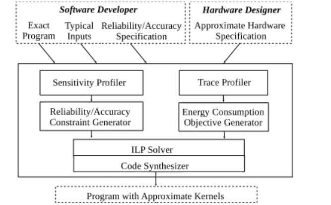
Figure

Documents relatifs
We also prove an additional result stating that approximate controllability from zero to con- stant states implies approximate controllability in L 2 , and the same holds true for
L’obligation de moyen pesant sur l’assuré social ne doit pas faire oublier que, de leur côté, les institutions de sécurité sociale sont soumises à l’obligation
L’archive ouverte pluridisciplinaire HAL, est destinée au dépôt et à la diffusion de documents scientifiques de niveau recherche, publiés ou non, émanant des
The aim of applying these additional criteria is to build an evaluation tree that minimizes the total computational cost of compiling (building the corresponding probability table)
To do so, the block by block elimination procedure (Bertel´e and Brioshi, 1972) relies on the tree decomposition characterization of the treewidth. The underlying idea is to apply
Cependant l’étude la plus importante réalisée à ce jour sur la colistine IV pour le traitement des infections à A.baumanii dans un service de réanimation a montré que
Ceci peut s’expliquer par le fait que les membres demeurent la partie la plus exposée aux traumatismes du fait de la présence des principaux os longs du corps, leurs
Histograms of Oriented Gra- dients (HOG) [6] is used as features for classification. We tested three types of approximations which are explained in Section 3. Exact RBF-kernel SVM
