Combining recognition and geometry for data-driven 3D reconstruction

Combining Recognition and Geometry for

Data-Driven 3D Reconstruction

by

Andrew Owens

Submitted to the Department of Electrical Engineering and Computer

Science

in partial fulfillment of the requirements for the degree of

Master of Science in Electrical Engineering and Computer Science

at the

MASSACHUSETTS INSTITUTE OF TECHNOLOGY

February 2013

©

Massachusetts Institute of Technology 2013. All rights reserved.

A u th o r ...

.

...

Department of Electrical Engineering and Computer Science

February 1,2013

Certified by.

William T. Freeman

Professor

Thesis Supervisor

Certified by...

...

/. ..

...

. ...

A ccepted by ...

//n,)

Antonio Torralba

Associate Professor

Thesis Supervisor

(Lesli

Combining Recognition and Geometry for Data-Driven 3D

Reconstruction

by

Andrew Owens

Submitted to the Department of Electrical Engineering and Computer Science on February 1, 2013, in partial fulfillment of the

requirements for the degree of

Master of Science in Electrical Engineering and Computer Science

Abstract

Today's multi-view 3D reconstruction techniques rely almost exclusively on depth cues that come from multiple view geometry. While these cues can be used to pro-duce highly accurate reconstructions, the resulting point clouds are often noisy and incomplete. Due to these issues, it may also be difficult to answer higher-level ques-tions about the geometry, such as whether two surfaces meet at a right angle or whether a surface is planar. Furthermore, state-of-the-art reconstruction techniques generally cannot learn from training data, so having the ground-truth geometry for one scene does not aid in reconstructing similar scenes.

In this work, we make two contributions toward data-driven 3D reconstruction. First, we present a dataset containing hundreds of RGBD videos that can be used as a source of training data for reconstruction algorithms. Second, we introduce the concept of the Shape Anchor, a region for which the combination of recognition and multiple view geometry allows us to accurately predict the latent, dense point cloud. We propose a technique to detect these regions and to predict their shapes, and we

demonstrate it on our dataset.

Thesis Supervisor: William T. Freeman

Title: Professor of Electrical Engineering and Computer Science Thesis Supervisor: Antonio Torralba

Acknowledgments

I would like to thank my advisors, Bill Freeman and Antonio Torralba for their invaluable advice, their patience, and for making the vision lab a productive and comfortable environment.

I would also like to thank Jianxiong Xiao. The work in this thesis was done in

collaboration with Jianxiong, and I have learned a lot from working with him. I also thank Joseph Lim, who I worked with on another project, and Sameer Agarwal, who hosted me during a very interesting and rewarding summer internship at Google.

I'd like to thank everyone in the vision group for the helpful discussions and for

the fun times both in and outside the lab: Roger, Donglai, Neal, Katie, Michael, Tianfan, YiChang, Hyun, Phillip, George, Ramesh, Andy, Christian, Adrian, Joseph, Jianxiong, Aditya, Carl, Tomasz, Zoya, and Hamed. I would also like to thank my roommate Abe Davis for his friendship and for all the fun times hanging out.

I had a wonderful experience learning to do computer vision research as an

un-dergraduate at Cornell. I would like to thank Dan Huttenlocher for introducing me to computer vision and research in general, Noah Snavely for introducing me to 3D reconstruction, and David Crandall for kindly and patiently helping me early on. I would also like to thank my mentor from even before that, David Kosbie, for, among other things, getting me on the right track with computer science.

Most of all, I'd like to thank my mother, Aileen, my sister, Christa, and my late father for their love and support over the years. I will always appreciate the sacrifices that my mother has, selflessly, made to help me along the way.

Contents

4.2 Shape Anchor Detection . . . . 21

5 Detecting Shape Anchors 23

5.1 Proposing Shape Candidates . . . . 23

5.2 Estimating Absolute Depth . . . . 24

5.3 Verifying Shape Candidates . . . . 25

6 Reasoning Across Multiple Views 27

6.1 Jointly Detecting Shape Anchors . . . . 27

7 Results 30

7.1 Experiment Setup. . . . . 30

7.3 A ccuracy . . . . 31

7.4 Qualitative Results . . . . 36

8 Conclusion 43

List of Figures

3-1 Examples from our database: each column contains four examples from

each place category. The numbers below the category names are the median example areas for each place category. . . . . 16 3-2 Place category distribution. . . . . 17 3-3 Dataset statistics. Refer to Section 3.2 for explanation. . . . . 19

4-1 Example Shape Anchors. Each match is displayed as a 2 x 2 figure, whose format is as follows. Upper left and bottom left: an image patch and its ground-truth depth map. Upper right and bottom right: the image and depth map of an exemplar patch with a similar shape (found

by our algorithm). Please see Figure 7-4 for more examples. . . . . . 22

7-1 Match results and multi-view stereo example. (a) The source patch

column shows the original patch, and the matched patch column shows a match from the dataset after the geometric verification step. Most predictions seem qualitatively correct, despite the sparsity of the multi-view stereo point cloud (b). . . . . 32 7-2 Error estimates for the shape predictions. All results are for the MAP

solution of the inference procedure. . . . . 34

7-4 Random, correct Shape Anchor detections. Each match is displayed as a 2 x 2 figure, whose format is as follows. Upper left and bottom left: original image patch and its ground-truth depth map. Upper right and bottom right: image and depth map of the exemplar patch from which the point cloud was transferred. Blue means

unknown depth. Depth is mean-centered. . . . . 37

7-5 Random, incorrect Shape Anchor detections. Please refer to Figure 7-4 for an

explanation of the format. . . . . 39

7-6 Shape Anchor predictions (1 of 3). We show a point cloud formed by taking the

union of all the shape predictions that for a given frame. To generate this diagram, we selected one or two frames from each reconstruction that (qualitatively) looked accurate. Points are colored by projecting them into the camera and using the color at that pixel. Note that the camera viewpoint has been moved from the original

location to better show the 3D structure. . . . . 40

7-7 Shape Anchor predictions (2 of 3). Please see Figure 7-6 for an

expla-n atioexpla-n . . . . 41

7-8 Shape Anchor predictions (3 of 3). Please see Figure 7-6 for an

Chapter 1

Introduction

In recent years, there has been exciting progress in building 3D models from multiple images. In this area, state-of-the-art techniques almost exclusively use depth cues that come from multiple view geometry and work by triangulating points that appear in multiple images. While this produces good results in many cases, these geometric depth cues have limitations, since the underlying problem of finding correspondences between images is difficult. Consequently, the resulting point clouds are often noisy and incomplete.

In this work, we describe a way to use techniques from recognition to overcome some of these problems. Our ultimate goal is to take a point cloud that comes from multi-view stereo [12] and then densify it in a few places where we can confidently predict the latent geometry. We do this in a data-driven way, using a large database of RGBD video sequences that we introduce.

In support of this goal, we introduce the idea of Shape Anchors. A Shape Anchor is an image region for which the combination of recognition cues and multiple view geometry allows us to confidently predict a dense, accurate point cloud. We formalize what we mean by predict and accurate in Chapter 4.

Our goal is to find Shape Anchors in videos, and our problem formulation some-what resembles an object detection problem, where Shape Anchors are the objects that we are looking for, and a correct point-cloud prediction is analogous to a correct object detection. Correct Shape Anchor detections provide information about

geom-etry that is useful and complementary to the triangulated points that they are partly derived from (although the depth estimates from Shape Anchor points are somewhat less accurate than those of triangulated points). Points that come from Shape An-chor predictions are dense compared to those generated by triangulation, such as those that come from the multi-view stereo technique we use in our experiments [12]. Furthermore, Shape Anchors can be detected in low-texture regions, where densely triangulating points is difficult. They can also provide qualitative information about the geometry that may not be obvious from just a sparse point cloud, such as the locations of occlusion boundaries and corners. In this way, Shape Anchors can po-tentially help confirm that there really is a crisp, 90-degree corner between the wall and the floor; whereas there is enough uncertainty in some sparse, multi-view point clouds that one might have to reluctantly admit the possibility that the two surfaces intersect in a more rounded way.

Our formulation is intended to be used in a high-precision, low-recall regime, in which we predict the geometry for only small number of regions in a scene, but when we do so, the geometry is likely to be accurate. This formulation can be used with current recognition techniques, which are themselves best suited for predicting with high precision and low recall. In this way, our approach is different from other recognition-based reconstruction techniques, which formulate depth-estimation as a regression problem and try to predict the depth of every pixel.

In this thesis, we describe a way of detecting Shape Anchors that involves searching a large database of RGBD videos (Chapter 5), then removing proposals that disagree with the sparse geometry provided by triangulated points. Finally, we describe how to remove Shape Anchor detections that are inconsistent with each other in Chapter

6.

We ' also introduce a dataset (Chapter 3) that is useful for developing data-driven reconstruction algorithms. Our dataset contains hundreds of RGBD videos, taken of real-world, indoor scenes. The videos in this dataset are recorded in a systematic way that allows for building dense, complete 3D reconstructions using RGBD-based

structure-from-motion techniques. This reconstruction can then be used as ground truth for techniques that do not have access to the depth data. We describe the dataset construction procedure and provide statistics about the dataset but omit information about the RGBD structure-from-motion algorithm in this thesis.

We apply the Shape Anchor-detection algorithm to this dataset (Chapter 7). In some cases, these predictions occur often and correctly enough to get a qualitatively correct, and fairly complete, reconstructions of some views. We also show many visualizations of the predictions to demonstrate their qualitative correctness.

Chapter 2

Related Work

2.1

Recognition-based 3D Reconstruction

3D reconstruction is a classic problem in computer vision, and recently

recognition-based techniques that use statistical techniques to build reconstructions of real-world

images from a single view have produced some impressive results. Early work in this area focused on recovering a very coarse reconstruction of a scene. Torralba and Oliva

[37] recovered the mean depth of a scene from a single image, and in parallel lines

of work, Hoiem et al. and Saxena et al. created planar reconstructions of outdoor scenes. Hoiem et al. estimate what they call qualitative aspects of a 3D scene [16] [17]

- the dominant surfaces, their surface orientations, and occlusion boundaries - from

which they construct a photo pop-up [18], a coarse piecewise-planar reconstruction that resembles a pop-up book. Meanwhile, Saxena et al. estimated per-pixel depth from a single image [28] in a Markov Random Field framework and in later work built piecewise-planar reconstructions [29] with a system called Make3D.

While these early techniques achieved impressive results, they use parametric models and are primarily limited to outdoor scenes with relatively simple geometry. In response to these limitations, Karsch et al. [19] recently introduced an interesting data-driven technique that involves transferring depth from similar-looking images using a technique based on SIFT Flow [21]. Their data-driven approach is appealing, because it may be better at capturing the variation in geometry of real-world scenes

than previous approaches. Our approach is similar to theirs in that it works by trans-ferring depth from a training set in a nonparametric way, but they transfer depth at an image level, while we transfer it closer to the object level. Unfortunately, we ex-pect image-level transfer (in the style of SIFT Flow) to have fundamental limitations, especially when the goal is to reconstruct real-world indoor scenes with fine detail. This is because the approach seems to require finding a pool of images to transfer from that contains exactly the right set of objects in exactly the right locations

There has also been recent work that exploits the special structure of indoor scenes. This line of work often makes heavy use of vanishing point cues, explicitly models walls, and detects objects in a categorical way. Delage et al. [7] build piecewise-planar reconstructions from a single image of a scene that obeys the Manhattan World assumption. Yu [38] model a scene as a set of depth-ordered planes and recover it in a bottom-up, edge-grouping framework. Hedau et al. [15] adapts the qualitative geometry idea to indoor scenes, modeling the walls with a box and the surfaces with a few coarse categories. Recently Satkin et al. [27] proposed a data-driven technique for reconstructing indoor scenes. Their technique uses a large collection containing thousands of synthetic 3D models that they obtain by searching for rooms categories like "bedroom" and "living room".

In contrast to this line of work, we make no explicit assumptions about the overall geometry of the room or the semantic categories of objects that it contains. Further-more, our dataset contains real-world scenes where the assumptions they make may not hold (e.g. images of non-rectangular rooms and up-close shots of objects).

We note that these recognition-based approaches all attempt to solve the very difficult problem of building a 3D reconstruction solely from recognition cues, while in our work we have access to multi-view information. In this way, our work is similar to [10], which proposes an elegant model for reconstructing a Manhattan World from a mixture of monocular and multiple-view cues. The goal of our work is very similar to that of [30], which extends the model from [29] to include triangulation cues. However,

'In our experience, nearest-neighbor search using features like GIST [24] is difficult for indoor scenes from our database, possibly for this same reason.

their ultimate goal is to build a piecewise-planar reconstruction of the whole scene, while ours is to recover a dense point cloud for a portion of the scene.

The approach that we use is similar to the "example-based" techniques of [11] and [5]. These techniques interpret a 3D shape by breaking the image into patches, searching for candidate shapes to fill each patch. They then, like us, use a Markov Random Field to enforce that depth predictions agree with one another where the patches overlap. Indeed, our work can be viewed as an adapation of this general idea to to real images. One key difference is that ours is more of a detection problem. They attempt to explain every patch in the image, while our goal is only to explain a subset of the patches that we are very confident about: a concession that we think makes sense for real images, where many patches are highly ambiguous.

There have been many recent papers in object detection that our work draws from. First, the idea of finding image patches whose appearance is informative about geometry is similar to that of poselets [3], visual patterns that are highly informative about human pose. Similarly, [33] describes finds mid-level discriminative patches that are in some way distinctive and representative of the visual world. This approach was subsequently used to find patches that are highly discriminative of the city in which a photo was taken [8]. Second, the idea of transferring meta-information from a training set was explored recently in [23], as was the idea of using a sliding window detector for image search [31]. Additionally, we use HOG [6] features and whiten them using

Linear Discriminant Analysis, as suggested by [14].

The goal of our work is very similar to that of multi-view stereo, and we use the state-of-the-art system [12] as part of our approach. Our work is similar in spirit to techniques that use appearance information to improve the shape estimates that come from stereo [36] [1]. And while there are existing techniques that can be used to densify point clouds, e.g. Poisson Surface Reconstruction [20], we are not aware of any that do so in a data-driven way for real-world scenes.

Finally, in Chapter 3 we introduce a dataset that is similar to the NYU RGBD Dataset [32], but our videos are recorded in a systematic way that makes it possible to build full 3D reconstructions using structure from motion.

Chapter 3

Dataset

In this chapter, we describe a dataset that is useful for data-driven 3D reconstruction. Our 1 dataset consists of full 3D models of indoor places (i.e. one or more adjacent rooms that a person can walk through), as demonstrated in Figure 3-1. Places in the dataset may be as small as a single bathroom or as large as an apartment. We collect this dataset by capturing an RGBD video of each place (Section 3.1).

We analyze the dataset's statistics in Section 3.2 and describe its usage for data-driven 3D reconstruction Section 3.3.

Our dataset has a number of desirable properties. First, it is very large, containing hundreds of videos. The videos cover a wide variety of places, but there are also a large number that come from the same or nearby buildings and consequently they share common object and architectural styles. This subset of videos may be useful for some applications, such as robotics. Second, our database is thorough: each place (e.g. conference room, apartment, laboratory) is captured systematically: operators try to make sure that the important viewpoints are well-represented and that the sequence can easily be reconstructed using R.GBD-structure-from-motion techniques. Third, our dataset is fully reconstructed: we apply an RGBD structure-from-motion algorithm to the videos (not described here), the results of which can be used as ground truth for R.GB-only reconstruction techniques, such as the one we describe in

apartment conf. room conf. hall restroom

57 ni2 47 m2 130 m2 23 m2

A - W.

classroom dorm hotel room lab lounge office

109 m2 33 m2 41 m2 55 n2 124 m2 49 n2

ga, 4

Figure 3-1: Examples from our database: each column contains four examples from each place category. The numbers below the category names are the median example areas for each place category.

the rest of this thesis.

3.1

Data Collection

Capturing procedure Each operator is told to capture the video mimicking

hu-man exploration of the space as much as possible. They are told to walk through the entire place, thoroughly scanning each room, capturing each object, the floor, and walls as completely as possible. The operators (five computer vision researchers) took special care to make the scans easier to reconstruct using structure-from-motion algorithms. Guidelines include walking slowly, keeping the sensor upright, avoiding textureless shots of walls and floors, and walking carefully between rooms to avoid reconstructions with disconnected components.

Capturing setup For the hardware, we tried the Microsoft Xbox Kinect sensor

and ASUS Xtion PRO LIVE sensor, both of which are available at low cost in the digital consumer market. While the Kinect sensor has a slightly better RGB camera,

corridor(5%)

others conference room(1 9%)

restroom (5%)

classroom(6%)

office(6%)

apartment(1 7%)

dorm(6%)

lounge(9%)

hotel(9%) lab(9%)

Figure 3-2: Place category distribution.

we used the USB-powered Xtion sensor for most scans, because it is more portable, and we can mount it to a laptop.

To make a database that closely matches the human visual experience, we want the RGBD video taken at a height and viewing angle similar to that of a human. Therefore, the operator carries the laptop with the Xtion sensor on his or her shoul-der with a viewing angle roughly corresponding to a horizontal view slightly tilted towards the ground. During recording, the operator sees a fullscreen R.GB image with registered depth superimposed in real-time to provide immediate visual feedback. We use OpenNI to record the video for both RGB and depth at 640 x 480 resolution with

30 frames per second. We use the default factory sensor calibration for the

registra-tion between the depth and image. The data is saved on disk without compression, on a powerful laptop with fast disk access (which is necessary to capture at a high frame rate). We scan only indoor places, because the RGBD cameras do not work under direct sunlight.

3.2

Dataset Analysis

We have 389 sequences captured for 254 different places, in 41 different buildings. Operators capture some places multiple times, at different times when possible. Ge-ographically, the places scanned are mainly distributed across North America and Europe.

We manually group them into 16 place categories (Figure 3-2). Some examples are shown in Figure 3-1, and the place category distribution is shown in Figure 3-2.

Figure 3-3 shows additional statistics of our dataset, where all the vertical axes represents the percentage of our dataset. Figure 3-3 (a) and (b) show the distribu-tion of sequence length and physical area of the space that was reconstructed in our dataset. Figure 3-3 (c)--(f) show the distribution of camera viewing angle, height, and the density of camera location in the space. From these statistics, we can see that our captured sequences satisfy our requirement to mostly mimic human visual experiences. Also Figure 3-3 (g) and (h) show that the camera was generally at least 2 meters away from the 3D scene, suggesting that our data seems to satisfy our ini-tial objective of resembling natural exploration of the environment. Figure 3-3 (i) illustrates the portion of area explored by the observer, by counting the number of square meters the observer walked on, divided by the total area of the room. Typi-cally, 25%-50% of the space is explored by the observer. Furthermore, one important characteristic of our dataset is that the same objects are visible from many different viewing angles. In Figure 3-3 (j) and (k), we plot the distribution of the coverage in

terms of view counts and view angles for the same place in space, which are repre-sented as voxels of size 0.1 x 0.1 m2 on the floor. The view angle is quantized into 5-degree bins. Since the RGBD camera relies on projecting an infrared light pattern, reflective objects and materials will sometimes return no depth. In Figure 3-3 (1), we plot the proportion of invalid area in the depth maps, which also contains the missing depth area due to the relative displacement of infrared projector and camera.

3.3

Dataset Usage

In the next chapters, we use this dataset to perform 3D reconstruction in a data-driven way. We construct a training set of 152 sequences, which is used in Chapter

5 to perform a nearest-neighbor search. For the experiments in Chapter 7, we select 9 sequences from those remaining as a test set (10 with one long sequence failing to

(a) 15%L 10% 5% 0 10000 2000 number of frames (30 fps) (g) 25% 20% 15% [ 10%[ 5% 0% 0 1 2 3 4 5 6 7 8 9 10

distance to surface (meter) 15%/6

15% 10%

10%[

0 100 200 300 0-60 -30 0 306090

area coverage (mete2 camera tilt angle (degree)

(h) ₍ 25% 15% 20%A 15% 1k 10% 5%[ 5% 0 1 2 3 4 5 6 7 8 9 10 25% 50% 75% 100%

mean distance to surface (meter) area explored by the observer

(d) 10%

90 -60 -30 0 30 60 90

camera roll angle (degree)

(j) 40% 30% 20% 10% b 0 1000 2000 34000400 # frames that a cell is visible

(e) 20% 15% 10% 5% -0 -0.5 1 1.5 2 2.5

camera height (meter)

(k) 25% 20% -15%j 10%-5% 0 10 20 3040 50 60 70 # viewing directions 15% 10% 5% 0 1000 2000 3000 4000 5000 # frames taken within 1m

(1) 40%-30% 20% 10% 0% 25% 50% 75% 100%

pixels with valid depth

Figure 3-3: Dataset statistics. Refer to Section 3.2 for explanation.

dataset, though we ensure that there are no places that appear in both the test set and the training set.

In the test set, we use the depth provided by the RGBD sensor to reconstruct

the camera pose using a structure-from-motion algorithm for RGBD sequences. 2

Once we have the camera pose, we use the depth only for evaluation purposes, as the ground truth.

2

We intend to replace this step with a standard structure-from-motion algorithm, such as Bundler [34], in future work.

Chapter 4

Problem Formulation

In this chapter, we introduce a new representation for appearance-based 3D recon-struction.

4.1

Shape Anchors

We are motivated by the observation that there are some image patches that are distinctive enough that a human can confidently predict their full 3D geometry. And furthermore, there are image patches where the geometry is ambiguous, but where knowing a few 3D points resolves this ambiguity. For example, the geometry of a completely white patch is ambiguous. At best, we can tell that it is statistically likely to be a planar region, possibly from a wall or a floor. But when we combine this knowledge with a few 3D points, we can predict its geometry precisely (e.g. by fitting the parameters of the plane). 1

In this work, we introduce the term Shape Anchor to refer to these kinds of patches.

A Shape Anchor is an image patch where multi-view geometry and recognition allows

us to predict the latent, dense point cloud. We use this name to suggest that these are the patches whose shapes we can predict the most reliably; in other words "sturdy" 'In practice, our algorithm is unlikely to be successful at predicting the geometry of these no-texture regions, because the recognition and 3D alignment are somewhat decoupled. The algorithm will only propose a point cloud derived from the most similar-looking patch in the dataset, which is

regions of our shape interpretation. We now define this idea more precisely.

Suppose I is an image patch and S is a sparse, noisy set of 3D points (e.g. obtained using multi-view stereo) that are visible in I (i.e. they project inside the rectangle containing I), and further suppose that the corresponding ground-truth point cloud is P. Then I is a Shape Anchor if we can use the combination of I and S to estimate a point cloud

Q

#(P, Q) < T, (4.1)

where

#(X, Y) = max(#P(X, Y), $)(Y, X)), (4.2) and

(X,Y)=1 x-minJ|x-y l . (4.3)

xx

We note that this error function is similar to the one minimized when aligning points with ICP

[2].

0.1 meters.

To further motivate the idea, we give some examples of Shape Anchors that our Shape Anchor detection algorithm correctly detected (Figure 4-1).

4.2

Shape Anchor Detection

The problem of predicting depth from images is sometimes formulated (e.g. in [29]

[19]) as a regression problem, where the goal is to estimate the depth at each pixel,

and the error metric penalizes per-pixel predictions based on how much they deviate from the ground truth. In contrast, our formulation of the problem has similarities with object detection. Here, Shape Anchors are analogous to the objects that we are trying to detect. A Shape Anchor-detection algorithm predicts the geometry for a number of patches in an image: we call these Shape Anchor predictions, and they

Figure 4-1: Example Shape Anchors. Each match is displayed as a 2 x 2 figure, whose format is as follows. Upper left and bottom left: an image patch and its ground-truth depth map. Upper right and bottom right: the image and depth map of an exemplar patch with a similar shape (found by our algorithm). Please see Figure 7-4 for more examples.

are analogous to object bounding-box predictions made by object detectors. Each Shape Anchor prediction is then judged as either being right or wrong (i.e. not given a continuous score).

In order to get the geometry, we assume that we are given the camera intrinsics and pose (in meters). We then triangulate points to obtain a sparse point cloud

(details described in Section 5.2). Our goal is then to use these video sequences and sparse point clouds to detect Shape Anchors. Each of these Shape Anchors gives us a dense point cloud for a small region of the video sequence, and in Chapter 7 we analyze these point-cloud predictions.

Chapter 5

Detecting Shape Anchors

In the previous chapter, we defined Shape Anchors. In this chapter, we describe how to detect them. We break the process down into two steps. The first step is based solely on appearance: we search a large database for similar-looking image patches and produce a candidate shape. In the second step, we use the 3D geometry to test whether the candidate shape fits the point cloud well, and to estimate the shape's absolute depth.

5.1

Proposing Shape Candidates

Given an image patch I, we propose a candidate shape, a point cloud that we hypoth-esize is most similar to that of I. To obtain the candidate shape for a given patch, we search a large RGBD database and find the most similar-looking example; that example's point cloud then becomes the candidate shape 1.

Our procedure resembles that of

[31].

1

We do not use any geometry in this stage, though doing so would likely improve results. In the subsequent step, we will allow the shape candidate to translate, so conceptually we are searching for

a set of points Q that is most similar to the ground-truth P despite a translation. In other words,

we want

min 4(P, {t + xIx E Q}) (5.1)

tcT

to be small, where # is defined as in Equation (4.2) and T is a set of translations that is determined

patches extracted from the input image. We convolve these detectors with images from the training set and choose the point cloud of the example with the highest score.

In more detail, we downsample the input image, compute HOG [6] using the implementation of [9], and extract every 8 x 8-cell template, each corresponding to a

170 x 170-pixel image patch. We whiten each patch with our implementation of Linear

Discriminant Analysis, as in [14] [13], which has been shown to improve discrimination in an object detection task. We search at multiple scales to enable matching with objects that are at a different absolute distance from the camera. To do this, we convolve each template with the HOG feature pyramid of images (using 5 levels per octave) in our training set, using only levels of the pyramid which result in detection windows whose width is between 0.5 and 1.5 times as large as that of the original

(170 x 170) patches. We perform convolution as a matrix multiplication between a

matrix containing every image window and another containing every template, as in the implementation of [23]. This data set consists of 152 sequences, and we sample every 10 frames for speed; in total we search 67,845 images. In addition to the highest-scoring example, we also retrieve the next four highest-highest-scoring examples, requiring each to be from a different sequence. These examples are used to help to remove erroneous matches in Section 5.3.

5.2

Estimating Absolute Depth

Obtaining a point cloud In our experiments, we assume that the true camera pose has been given (we use the pose provided by the dataset in Chapter 3). We then

generate a point cloud using the PMVS [12], a multi-view stereo system. To do this, we sample 100 frames from at most 4 meters away from the image that we want to reconstruct and pass them into PMVS as input. 2

2

Sometimes we want to use multiple frames from the same sequence. However, we still compute the point cloud this way - as many small reconstructions centered around each camera - to simplify the implementation. We can avoid having to process whole sequences (which can be thousands of frames long), and the reconstructions can be done in parallel.

Aligning the candidate with the point cloud Consider an image patch I, and

let v be the direction of the ray that passes between the center pixel of I and the camera center 3. Let M be the set of points from the sparse point cloud that project into the window of I. For a shape candidate C, we first center it on the origin by subtracting the 3D point located at the center pixel of the detection window (we call

this point Xcenter). Then we try to shift C along v in a way that best explains the

points in M, minimizing the objective function

ac = arg min %c(M, {av - Xcenter + X X E C}), (5.2)

ae[1,5]

where %c(X, _{Y) is the number of points in X that are within 0.1 meters of some} point in Y. We optimize this objective by performing a grid search on a, sampling with steps of size 0.025. From this, we compute the shifted shape, C' {aev

-Xcenter + X X E C}.

We experimented with more complex ways of aligning the candidate to the point cloud, including techniques based on ICP, and with allowing more degrees of free-dom (like rotation), but we found that these approaches did not significantly improve results. This might be because the multi-view point cloud does not sample points uniformly along the surface (e.g. high-texture regions may be over-represented), or be-cause these approaches allow the point cloud to deform in complex ways to optimally explain the data.

5.3

Verifying Shape Candidates

Once the shape candidate has been recentered, we use the sparse point cloud to test whether the geometry is correct, throwing out shape candidates that do not sufficiently explain the point cloud. We formulate this as a machine learning problem and train a Random Forest classifier [4] [26] to categorize a given shape candidate (using 300 trees as sub-estimators). Positive examples are shape candidates that

3

Specifically, if K is the camera intrinsics matrix and x is the center pixel in homogeneous coordinates, then v = K~x. In other words, this is the ray on which every point projects to x.

satisfy the conditions for being Shape Anchors, as defined in Equation (4.1). We train the classifier using the patches that come from approximately one fourth of the videos in the training set, sampling two frames from each.

We describe one representative type of feature that we use: histograms of nearest-neighbor distances. For a more complete list, please refer to Appendix A. We define

Hd(X, _{Y) to be the histogram, computed over points x E X, of mingEy ||x - YlI. We}

include as features Hd(M, C') and Hd(C', M), where C' is the recentered candidate shape and M is the point cloud.

Chapter 6

Reasoning Across Multiple Views

In this chapter, we describe how to detect Shape Anchors jointly across multiple views in a sequence.

6.1

Jointly Detecting Shape Anchors

Detecting Shape Anchors independently can lead to a high false positive rate. Many errors of this form can be detected by the fact that different Shape Anchors predict different depths for the same pixel. We can reduce errors of this form by detecting Shape Anchors jointly, choosing only a subset that agree with one another. We model this as a Markov Random Field (MRF) and detect the Shape Anchors by estimating its MAP using Loopy Belief Propagation [25]. We note that this formulation is similar to other example-based shape interpretation techniques, such as ShapeCollage [5] and

VISTA [11].

In the MRF, we construct a node for every patch (i.e. aligned shape candidate) that is labeled a positive example by the detector trained in Section 5.3 (which has a high false-positive rate unless a more stringent confidence threshold is chosen). The nodes take one of two labels: on or off. Nodes that are on after the optimization become the final Shape Anchor proposals.

We add an edge between every pair of patches that contains a matching SIFT [22] feature. To establish these correspondences, we match every pair of images

that are within 4 meters of each other and remove matches that fail to satisfy an epipolar constraint, using a ratio of 0.8 for the ratio test. We then form tracks, as is standard practice in structure from motion [35] and remove inconsistent tracks. More specifically, we create a feature-match graph whose nodes are features and edges are matching features. Tracks are the connected components of this graph, and we remove any track that contains two features that come from the same image.

Note that as a special case of the above procedure, any pair of patches that overlap in the same image will have an edge between them (assuming there is a SIFT feature in the overlapping region and that it does not get removed while forming tracks).

To do inference, we minimize the objective function for a pairwise MRF

U(xi) + V(xi, Xj), (6.1) {i,j}EE

where xi E {0, 1} is a binary variable that says whether the patch will be detected or not in the final result (i.e.off or on), and E is the set of edges in the graph.

The unary cost, U(xi), is meant to capture how well the patch agrees with the point cloud. We simply use

U(xi) = (b - si)xi, (6.2)

where si is an estimate of the probability that the patch is a positive example, as estimated by the Random Forest classifier in Section (5.3), and we set b = 0.7. Note

that when a patch has no edges, it will be labeled on if its score exceeds b. For the binary potential, we use

V(xi, xj) = (c + weij)xizX, (6.3)

where eij is an estimate of the inconsistency between the two patches. For this, we compute the distance between the 3D points for which there is a SIFT correspondence:

eij = min( 5Xk-X |, Td), (6.4)

where there are n SIFT matches, X' and X' are the predictions of the 3D point for SIFT correpondence k of image patches i and

j

SIFT features give a pixel correspondence between the two patches; correct matches

ought to give the same 3D prediction for the corresponding pixels. We set c = -0.025

(to give slightly better scores to pairs of patches that agree than isolated patches with

few edges), w = 0.1, and rd = 2.

We compute the MAP of this MRF using Loopy Belief Propagation, run for 20 iterations with a sequential message passing scheme. The parameters in the MRF (namely, b, c, and w) were set by grid search on a one-example training set, while trying to maximize the total number of correct detections minus twice the number of incorrect detections 2, where the correctness of detection is given by the criteria in

Equation 5.1.

1_{We limit the correspondences to be SIFT matches to avoid reasoning about occlusions. When}

two features match, we assume that they are the same physical point and don't have to consider the case where one occludes the other.

Chapter 7

Results

In the previous chapter, we described an MRF-based approach for removing incorrect Shape Anchor predictions. In this chapter, we analyze the results of this algorithm on several videos.

7.1

Experiment Setup

Dataset We run the Shape Anchor prediction algorithm described in Chapter 6 on each video of a test set containing 9 videos. We give each of these videos a name based on its place category (Section 3.2), such as conference room or office. As described in Section 5.2, we assume that the camera pose has been estimated correctly (using the ground truth given by our dataset). We then use a multi-view stereo system, PMVS [12], to obtain the initial, sparse point cloud. For each video, we used only one of every 25 frames and truncated the videos at frame 6000.

Instance Similarity The videos in the training and test set are of different physical

rooms, but there are many similarities between them. Since some of the videos are taken in different rooms of the same building, there are common architectural motifs, and objects are often of the same model (e.g. the same type of table appears in many

conference room videos). 1

In our experiments, videos that came from the conference room category in par-ticular were very similar to the conference room videos in the training set (though to our knowledge, they were not taken in the same physical rooms). 2 Note that the presence of these sequences likely increases the accuracy of our predictions overall.

Performance We use a small test set because on the current, unoptimized imple-mentation it takes a long time to process each video. It takes about 3-8 hours to process each video on a cluster of 144 cores (12 machines), with most of the time going into the nearest-neighbor search (which involves convolving up to 43,000 HOG templates with a large database of images).

7.2

Transfer

Unlike some other nonparametric transfer techniques (e.g. SIFT Flow-based [21]), our technique transfers a small amount of content from many different images that all, as a whole, look very different from the input image. To illustrate this, we have shown the Shape Anchor predictions for one image, prior to performing the MRF-based joint inference (but after the geometric verification step), in Figure 7-1.

7.3

Accuracy

Shape Anchor Prediction Accuracy In Figure 7-2 (a), we analyze the accuracy of the final Shape Anchor predictions on a per-prediction basis. More precisely, for each Shape Anchor prediction, we test whether the predicted shape agrees (as in Equation 4.1) with the ground-truth point cloud of the image it was detected in. 'There are also higher-level similarities, since many of the rooms are arranged the same way (e.g. conference rooms with chairs - of different models - in similar locations). However, our approach cannot exploit this kind of regularity (whereas a SIFT-flow-inspired technique like [19] might be better able to).

2_{Also, the random sample of videos that we use in our test set contains a large fraction of}

32

(a)

(b)

Figure 7-1: Match results and multi-view stereo example. (a) The source patch column shows the original patch, and the matched patch column shows a match from the dataset after the geometric verification step. Most predictions seem qualitatively

Note also that many Shape Anchors overlap because either they come from the same image or they appear in two images with similar viewpoints (please see Section 7.4 for detection examples).

Per-pixel Accuracy We also analyze the detections on a per-pixel basis in Figure 7-2 (b), which measures the disagreement between the ground-truth depth and the

predicted depth at each pixel.

More precisely, suppose Xest is a point that was predicted in image I and that Xest projects to pixel x (i.e. x = PXest where P is the projection matrix of I). Further suppose that Xgt is the ground-truth point at x. Then we estimate the error as ||Xgt - Xest |. 3 If two points project to the same pixel in the image, then we only consider the closer one, effectively removing the farther point from the reconstruction (modeling occlusion). We also ignore any point that projects to a pixel for which we do not have ground-truth depth and any point that projects outside the image.

We note that per-pixel error - although commonly used in recognition-based re-construction

[29]

of a chair leg (or some other thin structure), is misestimated by a few centimeters, this would result in very high per-pixel error.

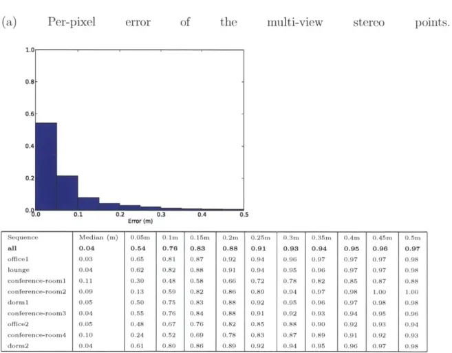
We also compute the per-pixel statistics for the multi-view stereo points them-selves, using the protocol above (Figure 7-3). We find that the multi-view stereo points are more accurate than the predictions on average. We do not consider this to be too surprising, given that the multi-view stereo points are used to predict the rest of the geometry, and that the dense Shape Anchor-derived points fill locations that (presumably) the multi-view stereo system was unable to triangulate.

Even though the depth error is worse compared to the multi-view results, we see in the qualitative results (Section 7.4) that seemingly important features of the geometry may be transferred that may not be obvious from the point cloud alone.

3

Ignoring discretization artifacts, the two points lie on the same ray entering the camera, so this quantity is equal to the absolute value of

IXgt

34

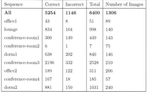
(a) Shape Anchor predictions: each patch evaluated as a whole. Number of patch shapes that were predicted correctly. Please see the text for more details.

Sequence Correct Incorrect Total Number of Images

All 5254 1146 6400 1306 officel 43 8 51 89 lounge 834 164 998 140 conference-room1 300 149 449 143 conference-room2 6 1 7 75 dormi 638 202 840 146 conference-room3 2196 332 2528 210 office2 189 122 311 206 conference-room4 167 18 185 57 dorm2 881 150 1031 240

(b) Per-pixel error. Histogram of pixel errors, in meters, computed over all sequences. 1.0 0.8 0.6 0.4 0.2 .0 0.1 0.2 0.3 0.4 0.5 Error (m)

Cumulative per-pixel error. Percent of pixels with error less than each threshold.

Sequence Median (m) 0.05m 0.1m 0.15m 0.2m 0.25m 0.3m 0.35m 0.4m 0.45m 0.5m all 0.10 0.27 0.51 0.68 0.78 0.84 0.88 0.90 0.93 0.94 0.95 officel 0.09 0.32 0.54 0.69 0.78 0.83 0.87 0.89 0.91 0.93 0.93 lounge 0.09 0.28 0.54 0.72 0.82 0.87 0.90 0.93 0.94 0.96 0.96 conference-roon1 0.14 0.18 0.38 0.54 0.66 0.75 0.81 0.85 0.88 0.90 0.92 conference-roon2 0.08 0.35 0.56 0.76 0.88 0.92 0.95 0.98 0.99 1.00 1.00 dorm1 0.14 0.20 0.38 0.53 0.64 0.72 0.79 0.84 0.89 0.93 0.95 conference-roon3 0.09 0.31 0.56 0.73 0.82 0.87 0.90 0.92 0.93 0.94 0.95 office2 0.13 0.19 0.37 0.56 0.70 0.79 0.85 0.88 0.90 0.92 0.93 conference-room4 0.07 0.37 0.63 0.79 0.87 0.90 0.92 0.94 0.94 0.95 0.95 dorm2 0.09 0.29 0.54 0.72 0.81 0.86 0.90 0.93 0.95 0.96 0.97

(a) Per-pixel _error of the multi-view 1.01 0.8- 0.6-0.1 0. 0.3 0.4 0.5 Error (m)

Sequence Median (m) 0.05m O.lm 0.15m 0.2n 0.25m 0.3m 0.35m 0.4m 0.45m 0.5m

all 0.04 0.54 0.76 0.83 0.88 0.91 0.93 0.94 0.95 0.96 0.97 officel 0.03 0.65 0.81 0.87 0.92 0.94 0.96 0.97 0.97 0.97 0.98 lounge 0.04 0.62 0.82 0.88 0.91 0.94 0.95 0.96 0.97 0.97 0.98 conference-room1 0.11 0.30 0.48 0.58 0.66 0.72 0.78 0.82 0.85 0.87 0.88 conference-room2 0.09 0.13 0.59 0.82 0.86 0.89 0.94 0.97 0.98 1.00 1.00 dorm 0.05 0.50 0.75 0.83 0.88 0.92 0.95 0.96 0.97 0.98 0.98 conference-room3 0.04 0.55 0.76 0,84 0.88 0.91 0.92 0.93 0.94 0.95 0.96 0ffice2 0.05 0.48 0.67 0.76 0.82 0.85 0.88 0.90 0.92 0.93 0.94 conference-room4 0.10 0.24 0.52 0.69 0.78 0.83 0.87 0.89 0.91 0.92 0.93 dorm2 0.04 0.61 0.80 0.86 0.89 0.92 0.94 0.95 0.96 0.97 0.98

Figure 7-3: Error of the multi-view stereo points

35

stereo points.

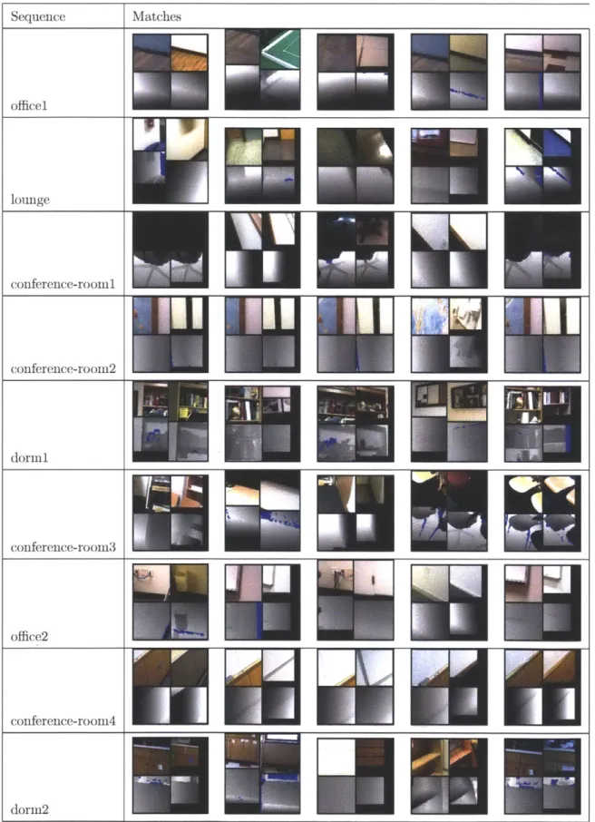
7.4

Qualitative Results

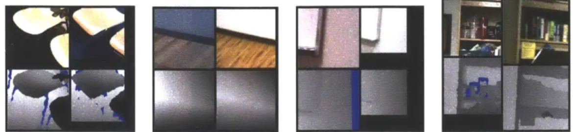
We show a random sample of correct (Figure 7-4) and incorrect (Figure 7-5) Shape Anchor predictions.

Many of the results that were marked as incorrect (and hence have an average per-point error that exceeds some threshold) nonetheless are "almost" right. There are some common reasons for these errors:

" In many cases, the multi-view point cloud contains errors, which leads to the

shape proposal becoming misaligned (Section 5.2). Note that these errors are not obvious in Figure 7-5, since the multiple-view point cloud is not shown.

" The orientation of a large object is predicted slightly incorrectly (e.g. a floor

being predicted with a slight slant).

" A prediction contains two layers, e.g. the edge of a table and the ground. The

error metric requires both to be predicted correctly.

These shortcomings suggest that the error measure that we use may be too strict.

Reconstructions We show some point clouds derived from Shape Anchor

predic-tions in Figure 7-6. There are several notable examples where the Shape Anchors provide qualitatively correct information that may not have been obvious from the sparse point cloud alone. For example, the office2 example predicts the geometry of the white wall correctly, but the point cloud seems to be sparse there (Figure 7-1

(b)). Similarly, the reconstruction at the edge of the door is reconstructed with fine

detail, but this level of detail does not seem to be present in the point cloud (on inspection). Two of the conference rooms, conference-roor3 and conference-room4 have fairly accurate and complete reconstructions. This is because there are similar (but not identical) rooms in the training set that we transfer the geometry from.

Finally, there are some notable failure cases. In conference-roomi, our algorithm seems to correctly predict that there are chairs there (transferred from a similar conference room), but the resulting reconstruction seems severely misaligned. The

37 Sequence officel lounge conference-room1 conference-room2 dorm1 conference-room3 Matches

U

,I[-U

U

dormi example transfers a wall that has the wrong surface orientation, and there is an artifact on the left edge of the bookshelf. Furthermore, while the algorithm is transferring geometry from other bookshelves (Figure 7-4), the alignment is incorrect, or the shelves look similar but in fact have different geometry (e.g. a different shelf pattern), making the resulting reconstruction look incorrect.

39 Sequence Matches office1 lounge conference-room1 conference-room2 dorm1 conference-room3 office2 conference-room4 dorm2

40

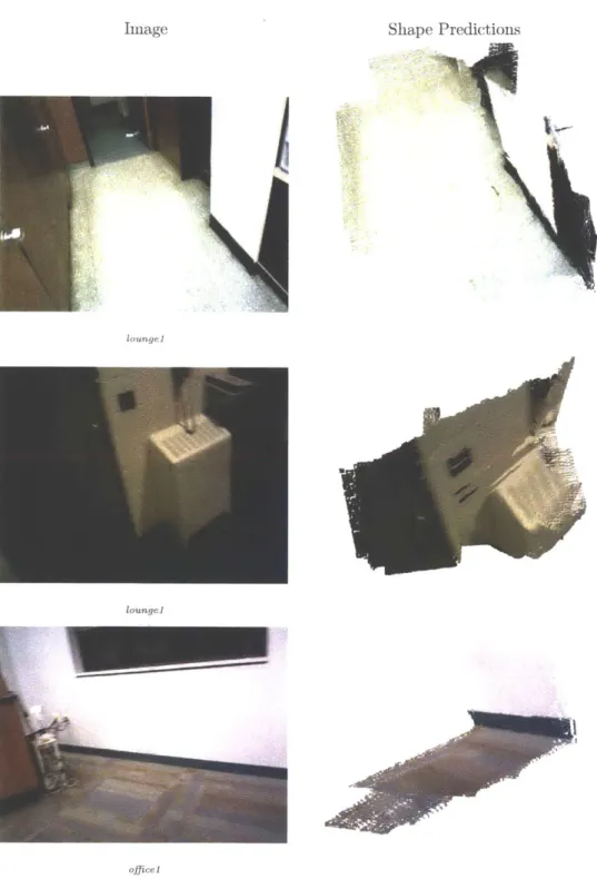
Image _{Shape Predictions}

lounge1

loungel

oicel

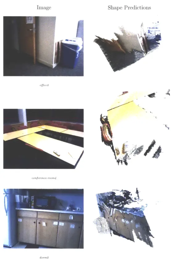
Figure 7-6: Shape Anchor predictions (1 of 3). We show a point cloud formed by taking the union of all the shape predictions that for a given frame. To generate this diagram, we selected one or two frames from each reconstruction that (qualitatively) looked accurate. Points are colored by projecting them into the camera and using the color at that pixel. Note that the camera viewpoint

41 conference-rooml conference-room2

b7

42 Shape Predictions -IL office2 conference-room4 dorm2

Figure 7-8: Shape Anchor predictions (3 of 3) Image

Chapter 8

Conclusion

We have explored ways of improving multi-view 3D reconstruction by using a combi-nation of multi-view geometry and recognition.

We introduce a large database of RGBD videos, along with their ground-truth 3D

reconstructions. These videos were recorded in a wide variety of locations and were captured so as to cover each place as much as possible.

We use this dataset to perform a new reconstruction task. We propose that

there are elements of a scene, called Shape Anchors, for which the combination of recognition and sparse multiple view geometry allows us to confidently predict the underlying, dense point cloud with low error.

We then describe a data-driven way of detecting Shape Anchors in videos where the camera pose has been estimated, and we have triangulated points. Given an image patch, we search a database of RGBD videos for the most similar-looking image patch (using only R.GB information), and then test whether the geometry of the retrieved match agrees with the sparse points. Matches that pass this test becomes Shape Anchor proposals, and we use an inference procedure that, jointly, distinguishes the good and bad proposals. Finally, we transfer the point clouds from the resulting Shape Anchor proposals into the scene, making a reconstruction that is denser in these high-confidence regions.

We analyze the accuracy of the fully reconstructed scenes and find that the pro-posed geometry has relatively low error (in the 0.1-meter range). Since the geometry

that comes from these predictions is dense, it can potentially provide useful high-level information that may not be as readily apparent from the point cloud alone.

We hope that in future work, we can use Shape Anchors to improve the metric accuracy of the reconstructed geometry. We would also like to explore how we can use Shape Anchors as the basis for growing a dense reconstruction, even in places where there are no Shape Anchor predictions.

Appendix A

Features used for Verifying Shape

Candidates

We include a list of features used to verify shape candidates, as described in Section

(5.3). We have omitted some features that were used in our experiments but which do

not seem to contribute much to the classifier's ability to discriminate between classes.

1. Convolution score.

2. Corig - Cdtn where crig is the center pixel of the rectangle containing the original

patch and Cdtn is that of the shape candidate's detection. This is to capture the

fact that the same object will look different depending on where in the image it appears. We also include the ratio between the area of the patch's area (in pixels) and the detection's area.

3. The number of points in the point cloud arid the number of quadrants of the

detection window that they cover.

4. An estimate of the matching error, using the point cloud as an estimate of the ground-truth shape:

#(M,

candidate shape, and

#

5. We define Hd(X, Y) to be the histogram, computed over points x E X, of

meters. We include as features Hd(M, C') and Hd(C', M).

6. We include a histogram that measures the similarity between the shape

candi-date and the next two candicandi-dates with the highest convolution scores (restricted

to be from different sequences).

jHd(C',

are the next two candidates, aligned using the procedure described in Section

5.2. And the reverse: !Hd(C2, C') + !Hd(C3, C').

7. _{The magnitude of the vector representing the translation used to align the points}

Bibliography

[1] J.T. Barron and J. Malik. High-frequency shape and albedo from shading using

natural image statistics. In Computer Vision and Pattern Recognition (CVPR),

2011 IEEE Conference on, pages 2521 -2528, june 2011.

[2] P.J. Besl and N.D. McKay. A method for registration of 3-d shapes. IEEE

Transactions on Pattern Analysis and Machine Intelligence, 14(2):239-256, 1992.

[3] Lubomir Bourdev and Jitendra Malik. Poselets: Body part detectors trained

using 3d human pose annotations. In International Conference on Computer

Vision (ICCV), 2009.

[4] L. Breiman. Random forests. Machine learning, 45(1):5-32, 2001.

[5] F. Cole, P. Isola, W.T. Freeman, F. Durand, and E.H. Adelson. Shapecollage:

occlusion-aware, example-based shape interpretation.

[6] N. Dalal and B. Triggs. Histograms of oriented gradients for human detection. In

Computer Vision and Pattern Recognition, 2005. CVPR 2005. IEEE Computer Society Conference on, volume 1, pages 886 893. IEEE, 2005.

[7] Erick Delage, Honglak Lee, and Andrew Y. Ng. Automatic single-image 3d

reconstructions of indoor manhattan world scenes. In In ISRR, 2005.

[8] Carl Doersch, Saurabh Singh, Abhinav Gupta, Josef Sivic, and Alexei A. Efros.

What makes paris look like paris? ACM Transactions on Graphics