HAL Id: hal-01202530
https://hal.archives-ouvertes.fr/hal-01202530
Submitted on 21 Sep 2015
HAL is a multi-disciplinary open access
archive for the deposit and dissemination of
sci-entific research documents, whether they are
pub-lished or not. The documents may come from
teaching and research institutions in France or
abroad, or from public or private research centers.
L’archive ouverte pluridisciplinaire HAL, est
destinée au dépôt et à la diffusion de documents
scientifiques de niveau recherche, publiés ou non,
émanant des établissements d’enseignement et de
recherche français ou étrangers, des laboratoires
publics ou privés.
Estimated by a Data-Driven Method
Timothée Gerber, Nadine Martin, Corinne Mailhes
To cite this version:
Timothée Gerber, Nadine Martin, Corinne Mailhes. Time-Frequency Tracking of Spectral
Struc-tures Estimated by a Data-Driven Method. IEEE Transactions on Industrial Electronics, Institute
of Electrical and Electronics Engineers, 2015, 52 (10), pp.6616-6626. �10.1109/TIE.2015.2458781�.
�hal-01202530�
Time-Frequency Tracking of Spectral Structures
Estimated by a Data-Driven Method
Timoth´ee Gerber, Nadine Martin, Member, IEEE and Corinne Mailhes, Member, IEEE
Abstract—The installation of a condition monitoring system aims to reduce the operating costs of the monitored system by applying a predictive maintenance strategy. However, a system-driven configuration of the condition monitoring system requires the knowledge of the system kinematics and could induce lots a false alarms because of predefined thresholds. The purpose of this paper is to propose a complete data-driven method to automatically generate system health indicators without any a priori on the monitored system or the acquired signals. This method is composed of two steps. First, every acquired signal is analysed: the spectral peaks are detected and then grouped in more complex structure as harmonic series or modulation sidebands. Then, a time-frequency tracking operation is applied on all available signals: the spectral peaks and the spectral structures are tracked over time and grouped in trajectories, which will be used to generate the system health indicators. The proposed method is tested on real-world signals coming from a wind turbine test rig. The detection of a harmonic series and a modulation sideband reports the birth of a fault on the main bearing inner ring. The evolution of the fault severity is characterised by three automatically generated health indicators and is confirmed by experts.
Index Terms—Condition monitoring, harmonics, sidebands, tracking, signal processing, fault diagnosis, wind turbines.
I. INTRODUCTION
C
ONDITION Monitoring Systems (CMS) are designed todetermine the health of a given system and to reduce the operating costs by allowing a predictive maintenance strategy. They are more and more commonly used, especially in wind turbines [1], [2] which have relatively high maintenance costs due to their hard-to-access remote location. The CMS allows to increase the energy efficiency of the wind turbine which makes it economically interesting. The hardware of a CMS is composed of sensors that acquire relevant signals. These signals are real-time analysed thanks to a computing unit which provides system health indicators. Two kind of analysis methods exist: the system-driven and the data-driven ones.The analysis methods which are the more frequently used are system-driven: the health indicators are defined depending on the monitored system kinematics. For example, in the case of bearing fault detection, standard indicators are computed by estimating the energy at the characteristic fault frequencies
Manuscript received September 30, 2014; revised March 27, 2015 and May 22, 2015; accepted June 19, 2015.
Copyright c 2015 IEEE. Personal use of this material is permitted. However, permission to use this material for any other purposes must be obtained from the IEEE by sending a request to [email protected]
T. Gerber and N. Martin are with Univ. Grenoble Alpes, GIPSA-Lab, F-38000 Grenoble, France and CNRS, GIPSA-Lab, F-F-38000 Grenoble, France (e-mail: {timothee.gerber, nadine.martin}@gipsa-lab.grenoble-inp.fr).
C. Mailhes is with Univ. Toulouse, IRIT / INP-ENSEEIHT, F-31000 Toulouse, France (e-mail: [email protected]).
(ball pass frequencies of the inner/outer ring, ball spin and cage frequencies). These indicators may be used for manual spectrum comparison [3], but also as features in data mining methods [4], [5] or in a probabilistic model [6] for the bearing diagnosis. In [7], a different part of the system is monitored (the rotor bar), but the approach is the same: the energy at the characteristic fault frequencies is estimated and used for the diagnosis. All these system-driven methods have a main drawback: each CMS has to be configured depending on the kinematics of the system to monitor. Moreover, a reconfiguration step is needed if a part of the system is changed after maintenance (e.g., replacement of a bearing by another one).
The second class of analysis methods is data-driven: the health indicators are derived from the data only, without any extra knowledge about the system. In [8], the empirical mode decomposition is used to extract features, then a classifier helps to diagnose the system health. However, the diagnosis is made on one measurement only, without considering the time evolution of the fault. In [9], the concept of intrinsic time-scale decomposition allows to deal with the non-stationarity in the system operations. At the end, the proposed indicators are time-frequency maps, which have to be manually inspected. Similarly in [10], the choice of the parameters for the multi-wavelet denoising is data-driven. The fault signature is isolated from the rest of the signal, but the time-domain signature has to be manually inspected or further processed to finally diag-nose the fault. In [11], [12], the wind turbine state variables are used to generate a residual which is then automatically thresholded to detect faults. However, the decision is binary and indicates if a fault is present or not, without providing more information. The same idea is used in [13], where more residuals are generated to identify precisely the defect at a cost of a more computationally consuming algorithm. Moreover, the number of sensors to monitor all the system inputs and outputs is high and costly.
We propose in this paper a complete generic and data-driven method without any a priori on the measured signals. This method does not need any configuration and is able to automatically provide system health indicators characterising the time evolution of a fault. In the case of a system part replacement, the indicators linked to the old part will simply stop and new indicators will automatically start.
The first step of the proposed method is to analyse each suc-cessive signal acquired at different timestamps. An automatic spectral analysis [14] detects and characterises the different spectral structures in the analysed signals and gives a snapshot of the system health. These spectral structures can either be single spectral peaks, or groups of peaks belonging to the
same harmonic series or to the same modulation sideband [15]. Each spectral structure is characterised by several parameters, including the number of peaks, the characteristic frequencies and the energy.
The second step consists of tracking the spectral structures through the different timestamps to create spectral structure trajectories from which health indicators will be derived. The tracking algorithm proposed in this paper is based on McAulay & Quatieri [16] method which has been originally designed for single peak tracking in speech signals. The method is adapted here to deal with more complex spectral structures such as harmonic series and modulation sidebands. Moreover, to make the method more robust against the possible non-detection of some spectral structures at isolated timestamps, a sleep state adapted from [17] is added. Finally, each parameter of the spectral structures grouped in one trajectory is monitored and its temporal evolution is used as a system health indicator.
The paper is organised as follows. The main problematics are detailed in Section II. In Section III, the identification of spectral peaks and structures is explained. A time-frequency tracking review in Section IV explains the choices which lead us to the proposed method of Section V. Section VI presents the experiments conducted on real-world signals acquired on a wind turbine test rig to validate the proposed method. Conclusions and perspectives are given in Section VII.
II. PROBLEM POSITION
To monitor a system, vibration or electrical sensors are placed on the system components where possible changes are indicative of a developing fault. Each sensor acquires NS signals of duration τn (in seconds) and denoted by sn where n is the signal index related to its timestamp tn defined as the beginning of the measurement (in operating hours). The analysis of the sequence {s1, . . . , sn, . . . , sNS
} characterizes the system evolution. Note that the time interval between two successive acquisitions at time tn and time tn+1 is not necessarily uniform and may vary from a few minutes to a few days, depending on the user settings and the operating system conditions.
In this paper we focus on the identification of the signal evolution in the spectral domain. For example, in the case of vibration signals acquired on a mechanical system, each part of the machine (a gear, a bearing, . . . ) generates spectral peaks in the vibration spectrum. The frequency and the number of peaks does not depend only on the system kinematics but also on the system wear. The spectral analysis is thus one way to evaluate the condition of a system.
A spectral analysis of a signal sn allows to identify all the peaks Pn
i present in the spectrum, with i being the peak index in the list of all the detected peaks sorted by increasing frequency. Part of these peaks are organised in more complex spectral structures as harmonic series Hn
i or modulation side-bands Mn
i. The identification of these spectral structures is a crucial step of our proposed method as it increases the amount of information about the system condition.
Between times tn and tn+1, the set of spectral peaks and structures will evolve according to the system operation and
condition. Let us assume that this evolution is bounded in an interval which width will be parametrised according to the spectral resolution of the spectral estimator. Thus, we propose to track each detected peak through all the signals and to record its trajectory TP. In this paper, the principle of trajectories is extended to harmonic series and modulation sidebands, whose trajectories TH and TM contain a high amount of information about the long-term system evolution, its wear and its possible failure.
In order to evaluate the condition evolution of a system, two main steps are required, (1) the detection and the esti-mation of peaks and spectral structures in signals, and (2) the tracking of these peaks and structures through all the available signals. The next section (III) presents shortly the proposed detection and estimation methods. Then, Section IV discusses about time-frequency tracking methods that explains the path we followed to propose the time-frequency tracking method detailed in Section V.
III. AUTOMATIC IDENTIFICATION OF SPECTRAL PEAKS AND STRUCTURES
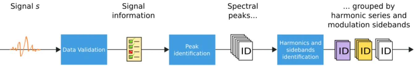
A CMS records signals of different types, like vibration, acoustic or electrical signals. In order to extract the spectral peaks and the spectral structures of those different signals in the same manner, we propose to use a generic and data-driven method based on an automatic spectrum analyser software conceived to be the easiest-to-use. In fact, each step of the spectrum analyser, illustrated in Fig. 1, is fully automatic and does not need any a priori knowledge or settings. The only action a user needs to do is to provide the signal to the spectrum analyser. Then, information are extracted from the signal to ease the peak detection. Finally, the list of detected peaks is scrolled to identify the spectral structures present in the spectrum. These steps are briefly explained afterwards. A. Data validation and peak identification
The method presented in this section is part of previous works [14], [18], [19] and is briefly explained here to ease the understanding of the paper.
The acquisition of each signal snis validated according to a procedure composed by four tests. This data validation checks that there is no signal saturation and that an anti-aliasing has been correctly used during the acquisition. Moreover, the data validation computes a global signal-to-noise ratio [19] and a non-stationarity rate [18], which should be null for a correct peak identification.
In the case of a non-stationary system like wind turbines, the acquisition process has been adapted to still get stationary signals. The acquisition is made continuously in a circular buffer, but the signal is only recorded once the non-stationarity rate computed on the buffer is lower than a predefined thresh-old (1% in our implementation). In the case where a rotation speed measurement is also acquired, the threshold is relaxed to a higher value (3%) and the non-stationarities are removed thanks to an angular resampling [20], [21], [22].
With this continuous acquisition system, the number of acquired signals is more than sufficient for wind turbine
Data Validation Signal s Spectral peaks... Harmonics and sidebands identification Peak identification Signal information ... grouped by harmonic series and modulation sidebands
ID
ID ID ID
Fig. 1. Illustration of the proposed automatic spectrum analyser and its different steps: from the input signal, data validation step collects information helping interpretation in the second step to detect all the spectral peaks which are finally grouped in harmonic series and modulation sidebands in the last step.
monitoring. Therefore, a second condition is used to trigger the signal recording: the wind speed has to take value within a given small range. As a consequence, the number of signals is reduced, but is still sufficient for condition monitoring purpose. More importantly, the signals are acquired in approximately the same operating conditions to allow the comparison of a signal to another.
Once the signal sn is acquired, the peak identification is done in the spectral domain. As defining an optimal spectral estimator for every kind of signals is hardly conceivable, a “multi-cycle” strategy is then proposed. This strategy uses multiple spectral estimators to take advantage of their different strengths [14]. The spectral estimators and their parameters are chosen thanks to the information provided by the data validation.
For each spectral estimator, a peak identification is per-formed directly on the spectral estimate. First, a series of peaks corresponding to maxima is extracted from the spectral estimate. Second, due to the estimation, it is clear that some of these peaks are only related to the estimation noise, while others are linked to the underlying signal. Thus, a statistical test is applied on each peak frequency (corresponding to the maximum of the peak) in order to decide whether this peak can be considered as an estimation noise peak or as a signal peak. Third, the detected signal peaks are then classified by comparing the spectral estimate with an over-sampled theo-retical spectral window related to the spectral estimator used. The objective of the comparison is twofold: first to characterise the spectral peaks and classify it in categories like: sinusoidal wave, narrowband signal or noise; second to increase the peak frequency precision by minimizing the quadratic error between the peak and the over-sampled window [14]. Performing these operations for one spectral estimator constitutes what we call one cycle.
Once every cycle is done, a fusion operation merges the results obtained by the different cycles and creates a unique ”spectral identity card” for each detected spectral peak Pi. The identity card is composed of several parameters characterising the detected spectral peak. Among them, one can find the estimated amplitude ai, the estimated frequency fi, and its associated uncertainty εiwhich is used in the spectral structure identification step. The uncertainty εi is linked to the spectral resolution of the estimators and means that the true frequency of the peak is in the interval [fi− εi, fi+ εi].
The final list of the detected peaks Pi is ordered by increasing frequency, with i ∈ J1, NPK being the index of the peak and NP being the total number of detected peaks.
B. Harmonic series identification
A harmonic series is a group of peaks which frequencies fi are multiple of a fundamental frequency νj. Methods to iden-tify harmonic series at the output of a spectral analysis exist in the literature; [23] proposed a method based on statistical tests with an a priori hypothesis which states that the power of the series is decisive for the detection. In [24], the diagnosis of a helicopter unit is done after harmonic identification thanks to an underlying model. However, these methods have been proposed for specific applications and the use of a priori prevents their use for a generic spectrum analyser. Moreover, the precision of the peak frequency estimation is limited and the uncertainty εidefined in Section III-A has to be taken into account during the harmonic search.
In this context, we propose to search the harmonics by frequency interval intersection. Each peak is considered as an interval and the interval has to overlap with the harmonic frequency interval model in order to be considered as a potential harmonic of rank r of the fundamental frequency νj
[fi− εi, fi+ εi]
| {z }
peak frequency
∩ [r(νj− εj), r(νj+ εj)]
| {z }
harmonic frequency model 6= ∅
with νj 6= 0 and r ∈ N∗. (1) If several peaks are candidates to be the rank-r harmonic, the peak with the nearest frequency fi to the model is selected
fi= arg min fkverifying (1)
|rνj− fk| (2)
Each time a peak is added in the harmonic series, the fundamental frequency νj and its uncertainty εj are refined in order to avoid a too large search interval for high ranked harmonics [15], [25]. Nevertheless, the method also allows harmonics to be absent including the fundamental frequency.
The search for harmonic series is made in an exhaustive way. Each detected peak Pi is considered as a potential fundamental frequency. If enough harmonics are found, the harmonic series Hj is then created and characterised. For example, the energy Ej of the series is computed and cor-responds to the sum of the peak squared amplitude. As for spectral peaks, an identity card is defined for every harmonic series
Hj ={{Pi|Pi verifies (1) and (2)}i∈J1,NPK, νj, εj, Ej} (3) The final list of harmonic series Hj is ordered in funda-mental frequency ascending order, with j ∈J1, NHK being the
index of the harmonic series and NH being the total number of detected series.
C. Modulation sideband identification
Modulation sidebands are peaks symmetrically and equally spaced around a carrier frequency νj. The frequency interval between the peaks is called the modulation frequency ∆j. Only the peaks which belong to at least one harmonic series are used as potential carrier frequencies. Around these poten-tial carrier frequencies, the search for modulation sidebands is exhaustive [15]. The frequency distances between one poten-tial carrier frequency and each detected peak in a modulation search interval are used as potential modulation frequencies. For each modulation frequency ∆j, if enough sidebands are found, the modulation Mj is then created.
As for harmonic series, the identification of the sidebands is made by frequency interval intersection
[fi− νj− εi, fi− νj+ εi]
| {z }
peak deviation from carrier frequency
∩ [r(∆j− εj), r(∆j+ εj)]
| {z }
modulation sideband model 6= ∅ with νj6= 0, ∆j6= 0 and r ∈ Z∗, (4) and in case of multiple candidates, the nearest one to the model is chosen
fi = arg min fkverifying (4)
|νj+ r∆j− fk|. (5) A specific identity card for each modulation sideband Mj is also defined, with j ∈ J1, NMK being the index of the modulation sideband and NM being the total number of modulation sidebands
Mj ={{Pi|Piverifies (4) and (5)}i∈J1,NPK, νj, ∆j, εj} (6) D. Discrete time-frequency map
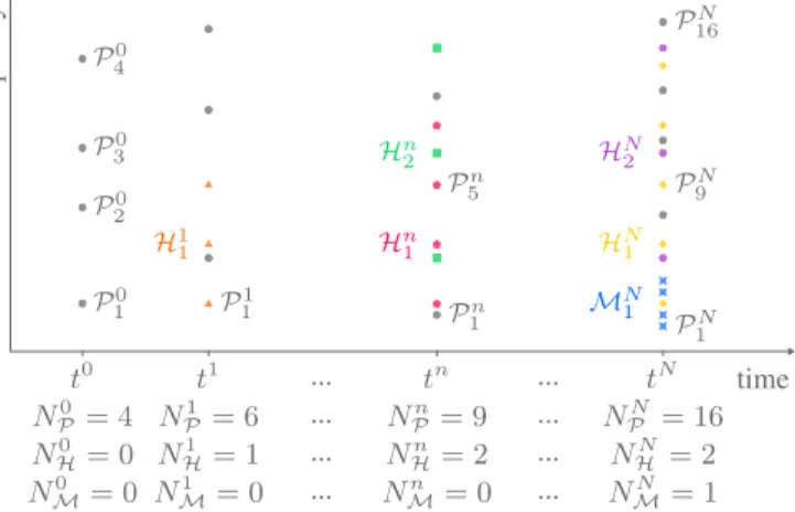
The identification of spectral peaks and structures is done on every signal sn acquired by the CMS. In the rest of the paper, the time index n will be added in the exponent position to every notation seen so far. For example, the frequency fn i of the peak Pn
i is the frequency of the ith peak detected in the spectrum of the signal sn. All the notations are illustrated in Fig. 2, which represents a time-frequency map where all detected peaks at each timestamp are represented by a marker which is a grey circle for remaining unassociated peaks, while peaks belonging to the same structure have the same color and shape. This map is discrete in both time and frequency. In time because the CMS records a signal on an irregular time basis when the system is in operation; in frequency because the spectral content is extracted from the spectrum.
IV. TIME-FREQUENCY TRACKING REVIEW
The problematic of time-frequency tracking is already present in the literature and several tracking methods exist. One of the most widely used is the one developed by McAulay & Quatieri [16], [17], [26], [27]. This method states that a peak
frequenc y time tn tN t1 t0 ... ... NPn= 9 NPN = 16 NP1 = 6 NP0 = 4 ... ... NHn = 2 NHN= 2 NH1 = 1 NH0 = 0 ... ... Nn M= 0 NMN = 1 N1 M= 0 N0 M= 0 ... ... P0 1 Pn 5 P0 2 P0 3 P0 4 PN 16 PN 1 P1 1 Pn 1 PN 9 H1 1 Hn1 HN1 Hn 2 HN2 MN 1
Fig. 2. Illustration of a time-frequency map obtained after spectral peak and structure identification for every signal acquired. Every detected peak is represented by a color and shape combination. Peaks belonging to the same spectral structure have the same color and shape, while peaks which are not in a spectral structure are represented by grey circles.
at time tn is associated to a peak at time tn+1if the frequency at time tn+1 is inside a search interval centered around the frequency at time tn. This simple but efficient method has been developed for peak tracking only. In [28], [29], [30], [31], they proposed to predict the future peak frequency at time tn+1 based on the peak trajectory in order to place the search interval around the predicted frequency. These methods improve the tracking of fast moving frequencies but need signals regularly acquired. All these peak tracking methods based on the work of McAulay & Quatieri are not only well suited to analyse audio signals but also for source separation or sound classification.
In [32], [33], a tracking method based on hidden Markov model is presented. The complexity of the resulting algorithms is high, which make them applicable only over short temporal period or in small spectral band. A maximum a posteriori estimation of one single trajectory has also been proposed in [34]; handling multiple trajectories might be possible if the trajectories are not overlapping. Another method [35], based on parsimony constraints and the Hungarian algorithm [36] tracks spectral lines in spectroscopy at the price of a high complexity.
Meanwhile, other kinds of methods track spectral structures which are groups of peaks representing harmonic series or modulation sidebands (as defined in previous section). It is particularly the case of pitch tracking methods where the pitch presents a harmonic structure. In [37], a spectral comb is designed to track the harmonic series of the signal pitch. An extension of the method allows to track two pitches at the same time, but only if their frequencies are not overlapped. In [38] the number of harmonic series tracked can be higher, thanks to a constrained classification method. However, the number of series is needed a priori.
In a CMS context, the tracking method should:
• be able to track both spectral peaks and spectral struc-tures,
information,
• be able to handle a significant amount of signals, with a large number of detected peaks in each signal (about thousands of peaks) and a high number of spectral structures (hundreds of them).
Therefore, the method should have a low complexity in order to avoid long computation time, and to be embedded in the CMS. To our knowledge, none of the previously cited methods verifies all these criteria. In that context, we propose a new tracking method as described in the next section. It is based on the one of McAulay & Quatieri we have adapted to track both peaks and spectral structures.
The McAulay & Quatieri method has been designed for audio signal analysis divided in short consecutive frames. The length of the frame is short enough (few tens of milliseconds) to consider the audio signal stationary over the frame. More-over, the frames are temporally contiguous. Thus, the signal content between two consecutive frames is almost the same, meaning that the peak frequencies are slightly evolving from one frame to another. This main hypothesis is the key of their tracking algorithm.
The context of condition monitoring is quite different from this one. The signal acquisition is generally not continuous to avoid collecting huge database. Moreover, the acquisition can be done on an irregular temporal basis. This means that the state of the system to monitor could be completely changed be-tween two signal acquisitions. This is troublesome, especially in rotating machines where characteristic frequencies of the system depend on the rotational speed. So, the main hypothesis to use the tracking algorithm in a condition monitoring context is to acquire the signals in a “constant machine state”, where the operational parameters do not change from one acquisition to the other. For example, the acquisition of signals on a rotating machine should always be done for the same rotational speed, or if not, an angular resampling [20], [21], [22] should be performed as a pre-process. In this case, the characteristic frequencies of the system will remain the same and the tracking will be possible.
V. TRACKING OF SPECTRAL PEAKS AND STRUCTURES
The method we propose tracks the spectral peaks and structures. It is based on the work of McAulay & Quatieri. Their peak tracking method and our proposed modifications will be explained just before describing how we propose to use it to track harmonic series and modulation sidebands. The tracking operations are organised in a specific order to monitor efficiently all the spectral content. Finally, thanks to this tracking, the health indicators are derived based on the estimated trajectories.
A. Tracking of spectral peaks
The peak tracking is done pairwise and sequentially; this means that for each pair of consecutive signals sn and sn+1, the peaks Pn
i detected in the signal sn (acquired at time instant tn) are associated with the peaks Pn+1
j detected in the signal sn+1(acquired at time instant tn+1> tn). This process is iterated for each signal index n ∈ J1, NsJ. Moreover,
the tracking is done peak by peak, starting from the low frequencies. Suppose that the tracking is done up to time tn and peak Pn
i−1. The next peak Pin has now to be linked with a peak at time tn+1 by a 2-step process detailed hereinafter, illustrated in Fig. 3 and resumed by (7).
Step 1: A candidate for the association is sought in a research interval ∆f. If there is no candidate like in Fig. 3(a), the trajectory of peak Pn
i dies. If there are multiple candidates, the one with the nearest frequency to fn
i is elected as the best candidate.
Step 2: The best candidate from step 1 has to verify the backward compatibility condition, i.e. the frequency of the candidate peak has to be nearer to fn
i than to any other detected peaks at time tn. If this backward condition is met, the association is done and the candidate is added to the trajectory of peak Pn
i (Fig. 3(b)). Otherwise, there are two cases; either, there is no more candidate in the search interval and the Pn
i trajectory dies (Fig. 3(c)), or there is at least one other candidate in the search interval and the association is done with it (peak Pn+1
j−1 in Fig. 3(d)).
The backward compatibility condition is satisfied when an association is valid forward and backward in time. The condi-tion to verify is expressed as δa < δb with δa = |fn
i − fjn+1| and δb = |fn
i+1− fjn+1|.
Note that all the peak parameters are known (estimated in Section III-A) and the only searching parameters to set is the search interval ∆f. In order to be as generic as possible, ∆f is chosen as a multiple of the spectral resolution, which only depends on the signal length and the spectral estimator. Empirically, ∆f has been chosen as 10 times the spectral resolution, which corresponds to the best compromise between the trajectory stability and a slight frequency evolution.
To sum up, the peak trajectories are constructed sequentially with Pjn+1∈ TP n i if fn i − ∆f 2 ≤ f n+1 j ≤ f n i − ∆f 2 with fn+1 j = arg min l=1,...,Nn P |fin− fln+1| and |fn i − fjn+1| < |fi+1n − fjn+1|. (7) In the original method proposed by McAulay & Quatieri, a third step considers the remaining unassociated peaks at time tn+1by starting new trajectories with them. However, this may induce trajectories composed of only one isolated peak, which increases artificially the total number of trajectories. To modify this third step we propose to create a new trajectory only if at least 2 successive peaks are included in it. The consequence of this modification is that some detected peaks may remain isolated and belong to none of the trajectories after the time-frequency tracking.
Moreover, the original method is not robust against a mis-estimated peak in frequency at a given time, as the trajectory directly dies. To solve this we propose to introduce a sleep state as described in [28]. It means that a trajectory can fall asleep and wake up, as long as the sleep duration is not too long. Otherwise, if the sleep duration exceeds a certain duration (2 successive processing temporal windows in our
(a) frequenc y time tn tn+1 ∆f (b) frequenc y time ∆f δb δa tn tn+1 Pn i+1 Pn i Pn i−1 Pj+1n+1 Pn+1 j Pn i+1 Pn i Pn i−1 Pj+1n+1 Pn+1 j−1 (c) (d) frequenc y time ∆f δb δa tn tn+1 frequenc y time ∆f δb δa tn tn+1 Pn+1 j Pn i+1 Pn i Pn i−1 Pn+1 j+1 Pj−1n+1 Pjn+1 Pn i+1 Pn i Pn i−1 Pn+1 j+1 Pn+1 j−1 Pn+1 j
Fig. 3. Tracking of the spectral peak Pn
i (in pink): (a) there is no peak in the
search interval ∆f, the trajectory dies; (b) the only peak in the search interval verifies the backward compatibility condition δa < δb, the peak Pn+1
j is
therefore associated to Pn
i trajectory; (c) the only peak in the search interval
does not verify the backward compatibility condition, the trajectory dies; (d) the nearest peak does not verify the backward compatibility condition, the association is then done with the peak Pn+1
j−1, also present in the search
interval.
context), the trajectory finally dies. This principle is illustrated in Fig. 4. tn frequenc y time tn−1 tn+1 tn−2 tn−3 tn−4
Fig. 4. Illustration of the sleep state used in the proposed method. The tracking is done up to time tn. Spectral peaks are represented by circles,
active trajectories by solid line and sleeping trajectories by dotted line. The green trajectory is definitively dead; the end of its sleep state is symbolised by a cross.
The tracking algorithm proposed here requires simple oper-ations and can, therefore, deal with a high dimension of peaks and signals. In fact, as the lists of peaks are already sorted, the peak frequency comparisons between too consecutive instants tn and tn+1need to run through each list only one time. This means that if the mean number of peaks per signal is NP, then approximatively 2 × NP comparisons are made for each
signal iteration, leading to a complexity in O(NsNP), where Ns represents the total number of signals.
B. Tracking of harmonic series
There are multiple possibilities in order to track harmonic series through time. In [39], each peak trajectory is inde-pendently tracked and the harmonic series are constructed afterwards by grouping the appropriated trajectories. In [37], [28], constraints of harmonicity are used during the tracking operation; however, only one or two harmonic series can be retrieved.
The method proposed in this paper relies on the fact that the peaks at a given time are already grouped in harmonic series Hn
i of fundamental frequency νni (see III-B). To capitalize this previous analysis, the tracking of harmonic series is done globally, meaning that when a harmonic series at time tn is associated to another harmonic series at time tn+1, the peaks inside the series are automatically tracked according to their rank in the series. If the rank-r harmonic is present in the series at time tn, but is not at time tn+1, the trajectory goes to a sleep state.
In order to track harmonic series, the peak tracking strategy described in section V-A is applied to the set of fundamental frequencies of all harmonic series Hn
i. This structural ap-proach is illustrated in Fig. 5, which highlights the robustness of the proposed global approach; the tracking is efficient even if the peaks are missing in the harmonic series and even if the fundamental frequency is been detected.
C. Tracking of modulation sidebands
The tracking of modulation sidebands seems a little more complex because each modulation sideband Mn
i is charac-terised by two parameters to track, the carrier frequency νn
i and the modulation frequency ∆ni. However, the carrier frequency is already tracked during the harmonic series track-ing. In fact, as explained in III-C, each carrier frequency is necessarily a peak belonging to a harmonic series. So, the peak trajectories TP constructed during the harmonic series tracking correspond already to the carrier frequency trajectories.
It is then possible to track modulation sidebands inside each carrier frequency trajectories thanks to the method presented in V-A. The peaks are replaced by the modulation sidebands around the carrier frequency trajectory, and the peak frequency by the modulation frequency ∆n
i of sidebands.
As for harmonic series, a modulation sideband is a group of peaks. Once a modulation sideband is tracked between two times tn and tn+1, the peaks inside the modulation are automatically tracked according to their modulation frequency. D. Feature extraction
Trajectories of different spectral structures have been iden-tified. From these trajectories and according to the type of spectral structure, trends are automatically derived by link-ing the characteristics associated to each spectral structures (see (3) and (6)). Thus, in the case of harmonic trajectories,
(a) t (b) n+1 frequenc y time tn tn+1 frequenc y time tn (c) t (d) n+1 tn frequenc y time tn tn+1 frequenc y time
Fig. 5. Tracking of harmonic series. Spectral peaks are represented by circles while fundamental frequencies are represented by squares. (a) Peaks belonging to the same harmonic series have the same color. Grey peaks do not belong to any harmonic series. (b) Harmonic series are now represented by their fundamental frequencies. (c) The tracking of fundamental frequencies is done; the harmonic series associated take the same color. (d) The peaks in harmonic series are automatically tracked according to their rank in the harmonic series. The line is solid if the rank is present in both harmonic series at times tn
and tn+1, otherwise the line is dotted.
the number of harmonics in the series, the energy and the fundamental frequency are used as system health indicators. The indicators derived from a modulation trajectory will be similar: the number of sidebands in the modulation, the energy and the modulation frequency. Examples of these indicators are given in the last section of the paper.
E. Full tracking algorithm
In order to track all the spectral content without redundancy in the peak tracking, our method is organised as follows: (1) identification of the harmonic series trajectories TH (Sec-tion V-B), (2) identifica(Sec-tion of the modula(Sec-tion sideband tra-jectories TM(Section V-C) and (3) tracking of the remaining peaks (Section V-A). The so-called remaining peaks are the peaks which after harmonic series and modulation sidebands tracking are not yet in any trajectories. Then, the final step consists in (4) extracting system health indicators from the identified spectral structure trajectories (Section V-D).
As the tracking algorithm works in a sequential way, it is easy to process the data online. Each time a new signal is acquired, steps (1), (2) and (3) are iterated on this new signal
to extend the trajectories. Then, step (4) updates the system health indicators.
VI. EXPERIMENTS
The proposed tracking method has been tested on real-world signals recorded over a wind turbine test rig, developed within the frame of the KAStrion project. This section starts with a brief introduction of the wind turbine test rig in VI-A, and ends up with the obtained results, already presented in [40]. The first main bearing has been dismantled after the first signs of the fault, while the second main bearing has been fully damaged up to totally stop the normal operation of the rig. These results are presented in VI-B and VI-C respectively. A. Experimental set-up: the wind turbine test rig
The test rig based on a wind turbine kinematics is designed at a smaller scale (10 kW). Instead of the blades, a geared-motor generates the main shaft rotation (around 20 RPM). A multiplier increases the rotational speed with a ratio of 100:1, allowing the generator to operate around 2000 RPM.
To accelerate the wear phenomena, the main shaft bear-ing can be loaded with axial and radial forces. Moreover, the test rig can run in two modes: the deterioration mode and the measurement mode. The working conditions for the deterioration mode are non-stationary, as the motor speed is programmed to simulate real wind speed profiles in order to apply more realistic constraints on the mechanical elements. On the contrary, during the measurement mode, the working conditions are stationary to immediately meet the constant machine state hypothesis. Measurements in non-stationary conditions are also possible but requires pre-processings as described in III-A to meet the needed hypothesis for the tracking operations.
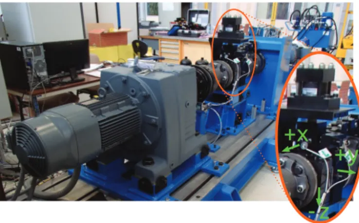
The test rig is an experimental platform monitored thanks to several sensors, including accelerometers, thermocouples, torquemeters, tachometers, voltage and current probes. This exhaustive monitoring allows to test different diagnosis meth-ods (not only the one described in this paper). For example, in [41] the voltages and currents are used for the electrical diagnosis of the test rig, while in [42] they are used for detecting rotor eccentricities. To test the method proposed in this paper, we will focus on 3 accelerometers taking place on the main bearing; one accelerometer in the axial direction (+x) and the other two in the radial direction (+y and −z). Fig. 6 illustrates the position and the directions of the accelerometers. The vibration signals are acquired while the test rig working conditions are stationary. The conditions remain the same throughout all the acquisition times. The hypothesis of con-stant machine state is therefore met. The vibration signals are acquired at different timestamps tn of the main bearing life (counted in operating hours) and the signal duration is the same for each acquisition: ∀n, τn= 150seconds. The signals are acquired at a sampling frequency of 39062.5 Hz, chosen as high as possible in this experimental setup to avoid loosing any high frequency information that might appear. However, a lower sampling frequency would still have been enough to monitor the test rig.
+x
+y
-z
Fig. 6. A picture of the wind turbine test rig. The orange ellipsis circles the main bearing and its loading unit, while the green arrows represents the 3 wired accelerometers and their respective directions. (+x) and (+y) sensors are visible in the zoom, while (−z) sensor is hidden below the main bearing.
B. Medium degradation of the main bearing
Each of the 3 accelerometers recorded 12 vibration signals during the main bearing wear test. On average for each signal, 19400 peaks were detected and grouped in 750 harmonic series and 21500 sidebands. If these numbers seem large, one has to remember that the identification methods of Section III are applied without any a priori on the signals. In this context, the detection thresholds are voluntary low in order to avoid missing any peak or structure. However, the number of identified structures could be decreased by providing the system kinematics.
For the radial accelerometer in the (−z) direction, the track-ing operations created 1084 harmonic series trajectories, 564 modulation sideband trajectories and 9327 trajectories among the remaining peaks. From each of these trajectories, trends are automatically generated according to the characteristics of the tracked structure.
One trajectory deserves a particular attention: a harmonic series trajectories with a sudden increase in energy around 203 operating hours. The fundamental frequency of this trajectory is 2.72 Hz and the harmonic series energy, shown in Fig. 7, evolves from 0.011 up to 1.6 µm2.s−2. Such an important increase in energy is characteristic of a fault.
So far, the proposed method managed to create without any a priori a system health indicator which detects the fault. To complete the diagnosis, information about the system kinematics is necessary in order to identify the mechanical part concerned. In this experiment, such information is available and indicates that the 2.72 Hz frequency corresponds to the ball pass frequency of the outer ring.
The wear test has been stopped after 214 operating hours. The rig was still able to operate, but the main bearing has been dismantled for visual inspection in order to visualize a fault in its early stage. The relevancy of the health indicator generated automatically has been confirmed by the presence of 3 small flakings on the main bearing outer ring.
This interesting system health indicator is part of a long list of generated indicators. In order to deal with this long list,
20 40 60 80 100 120 140 160 180 200 220
Time (in operating hours)
Ener gy (µm 2.s − 2) 0 0.6 1.2 1.8
Fig. 7. Evolution of the energy in the harmonic series at 2.72 Hz. After 203 operating hours, the energy starts increasing drastically.
the following reasonable hypothesis is made: the indicators computed on a healthy system will not vary much, while the indicators computed on a faulty system will evolve drastically. Accordingly, for a full automatic system health diagnosis, fur-ther work will focus on identifying automatically the evolving indicators which are the most interesting ones. The use of asymmetry or relative increase coefficients on the indicators show some potential for classifying the indicators, but has to be further developed.
The results of the other radial accelerometer (+y) and the axial one (+x) for this wear test will not be presented here as they show high similarity to that of the radial accelerometer (−z) and they confirm the already presented diagnosis. C. Full degradation of the main bearing
In this second experiment, a second main bearing, with a different kinematics, has been highly damaged up to totally stop the normal operation of the rig. At the end of the wear test, the main bearing has been disassembled and visually inspected.
For the accelerometer in the +y direction, 17 vibration signals were recorded while the main bearing wear. For each signal, the number of detected peaks is varying around 19000. These peaks are organized in approximately 600 harmonic series and 12000 modulation sidebands, thanks to the methods presented in Section III. After the tracking operations, we get 828 harmonic series trajectories and 9373 modulation sideband trajectories. Among the remaining peaks, 12406 trajectories have been created.
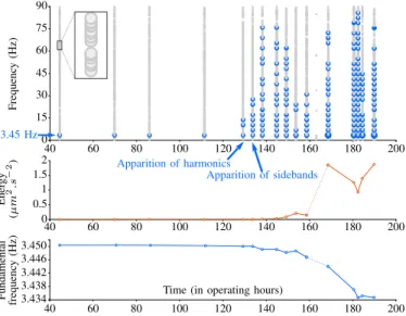
One of the trajectories deserves a special attention. It can be observed on the top of Fig. 8 which represents a discrete time-frequency map where all the detected peaks are symbolised by small grey circles. The top left corner zoom illustrates the peak density. Among these detected peaks, a particular peak at 3.45 Hz is tracked from 44 to 189 operating hours and is represented by bigger blue circles. Around 129 hours, this particular peak evolves to become a harmonic series with more and more peaks (see the increasing number of blue circles over time). The increasing energy of this trajectory is plotted in the middle of Fig. 8. Besides, the frequency of the trajectory is slightly decreasing (bottom of Fig. 8).
Moreover, shortly after the transformation of the peak at 3.45 Hz in a harmonic series, modulation sidebands started to appear. A 0.333 Hz modulation frequency around the 3.45 Hz carrier frequency is detected. It is shown in Fig. 9 that since the apparition of sidebands after 134 operating hours, their number increases accordingly to the severity of the fault.
40 60 80 100 120 140 160 180 200 0 0.5 1 1.52 Ener gy (µm 2.s − 2) 40 60 80 100 120 140 160 180 200 Frequenc y (Hz) 0 15 30 45 60 75 90 40 60 80 100 120 140 160 180 200 3.434 3.438 3.442 3.446 3.450 Fundamental frequenc y (Hz)
Time (in operating hours) 3.45 Hz
Apparition of harmonics
Apparition of sidebands
Fig. 8. Evolution of the inner ring fault on the main bearing, seen by a radial accelerometer. On the top, all detected peaks are represented by small grey circles on the time-frequency map. Blue and bigger circles belongs to the same harmonic series trajectory linked to the main bearing fault. Below, two trends of the harmonic series are plotted: the energy increases while the fundamental frequency is slightly decreasing.
Time (in operating hours)
40 60 80 100 120 140 160 180 200 6 10 14 18 Number of sidebands
Fig. 9. Evolution of the number of modulation sidebands around the slowly evolving carrier frequency starting at 3.45 Hz. The modulation frequency is equal to 0.333 Hz.
This 3.45 Hz frequency corresponds to the ball pass fre-quency of the inner ring. The apparition of harmonics and sidebands at 129 and 134 operating hours respectively are first signals of a fault birth. The increase in both the energy and the number of sidebands characterises the evolution of the fault and its severity. This increase in energy is distributed over the fundamental frequency and all its harmonics [43], hence the increasing number of detected peaks in the series as they start to have a higher level than the noise spectrum. Finally, the slightly decreasing frequency is another characteristic of a bearing fault and is explained by the fact that the inner ring wear generates slipping.
Another harmonic series trajectory deserves also some at-tention. As illustrated in Fig. 10, the energy of the series starts increasing around 144 operating hours, that is 15 hours after the first signs of the fault on the inner ring. The fundamental frequency of this series is 2.54 Hz and corresponds to the ball pass frequency of the outer ring. This increase indicates that the severity of the fault is becoming more and more serious as the fault is spreading from the inner to the outer ring.
The combination of these four automatically generated indicators (the energy and the frequency of the harmonic series at 3.45 Hz, the number of sidebands around the carrier frequency 3.45 Hz and the energy of the harmonic series at 2.54 Hz) mirrors out the failure and confirms the value of the
40 60 80 100 120 140 160 180 200
Time (in operating hours)
Ener gy (µm 2.s − 2) 0 0.03 0.06 0.09 0.12
Fig. 10. After 145 operating hours, the fault is propagated: the energy of the outer ring harmonic series is also increasing.
proposed method that works in a data-driven way.
It is also possible to see on Fig. 8 and 9 that around 163 hours, the harmonic series is not detected. In fact, this signal was highly non-stationary due to a high impulse in the vibrations. As a consequence, the spectral analysis was not able to identify correctly the spectral peaks and structures for this particular signal. However, the tracking of the harmonic series was not stopped, thanks to the sleep state. The sleep state on the energy, the frequency and the number of modulation curves is represented by a dotted line.
VII. CONCLUSIONS
A data-driven method producing system health indicators is proposed in this paper. The method is composed of two main steps. First, the spectral content of each signal is identified without any a priori on the monitored system or the acquired signals. The spectral peaks are identified and grouped in struc-ture as harmonic series or modulation sidebands. Secondly, these spectral peaks and structures are tracked through all the available signals. The trajectories constructed during the track-ing phase are finally used to automatically generate system health indicators from the structure estimated parameters.
The proposed method is tested and validated on real-world signals, acquired on a wind turbine test rig. The degradation of the main bearing confirmed by mechanical experts, has been detected in its early stage by the apparition of a harmonic series and a modulation sideband. The evolution of the fault severity is characterised by three automatically generated health indicators.
Future work will focus on sorting and classifying the generated indicators in order to move forward for a full generic and automatic tool to diagnose a system.
ACKNOWLEDGMENT
The authors would like to thank the CETIM, partner of the KAStrion project, for providing the signals coming from the wind turbine test rig.
The KAStrion project has been supported by KIC InnoEn-ergy, a company supported by the European Institute of Inno-vation and Technology (EIT), and has the mission of delivering commercial products and services, new businesses, innovators and entrepreneurs in the field of sustainable energy through the integration of higher education, research, entrepreneurs and business companies.
REFERENCES
[1] B. Lu, Y. Li, X. Wu, and Z. Yang, “A review of recent advances in wind turbine condition monitoring and fault diagnosis,” IEEE Conf. Power Electronics and Machines in Wind Applications, 2009.
[2] P. F. G. M´arquez, A. M. Tobias, M. J. P. P´erez, and M. Papaelias, “Condition monitoring of wind turbines: Techniques and methods,” Renewable Energy, vol. 46, pp. 169–178, 2012.
[3] X. Gong and W. Qiao, “Bearing Fault Diagnosis for Direct-Drive Wind Turbines via Current Demodulated Signals,” IEEE Trans. Ind. Electron., vol. 60, no. 8, pp. 3419–3428, 2013.
[4] D. He, R. Li, and J. Zhu, “Plastic bearing fault diagnosis based on a two-step data mining approach,” IEEE Trans. Ind. Electron., vol. 60, no. 8, pp. 3429–3440, 2013.
[5] T. W. Rauber, F. de Assis Boldt, and F. M. Varejao, “Heterogeneous Fea-ture Models and FeaFea-ture Selection Applied to Bearing Fault Diagnosis,” IEEE Trans. Ind. Electron., vol. 62, no. 1, pp. 637–646, 2015. [6] B. Zhang, C. Sconyers, C. Byington, R. Patrick, M. E. Orchard, and
G. Vachtsevanos, “A Probabilistic Fault Detection Approach : Applica-tion to Bearing Fault DetecApplica-tion,” IEEE Trans. Ind. Electron., vol. 58, no. 5, pp. 2011–2018, 2011.
[7] Y. H. Kim, Y. W. Youn, D. H. Hwang, J. H. Sun, and D. S. Kang, “High-resolution parameter estimation method to identify broken rotor bar faults in induction motors,” IEEE Trans. Ind. Electron., vol. 60, no. 9, pp. 4103–4117, 2013.
[8] J. Hang, J. Zhang, and M. Cheng, “Fault diagnosis of wind turbine based on multi-sensors information fusion technology,” IET Renewable Power Generation, vol. 8, no. 3, pp. 289–298, 2014.
[9] R. Court, P. J. Tavner, C. Little, and W. Yang, “Data-driven technique for interpreting wind turbine condition monitoring signals,” IET Renewable Power Generation, no. May 2013, pp. 151–159, Oct. 2013. [10] H. Sun, Y. Zi, and Z. He, “Wind turbine fault detection using multiwavelet denoising with the data-driven block threshold,” Applied Acoustics, vol. 77, no. 0, pp. 122–129, 2014.
[11] S. Yin, S. X. Ding, X. Xie, and H. Luo, “A review on basic data-driven approaches for industrial process monitoring,” IEEE Trans. Ind. Electron., vol. 61, no. 11, pp. 6414–6428, 2014.
[12] S. Yin, G. Wang, and H. R. Karimi, “Data-driven design of robust fault detection system for wind turbines,” Mechatronics, vol. 24, no. 4, pp. 298–306, 2014.
[13] S. X. Ding, P. Zhang, A. Naik, E. L. Ding, and B. Huang, “Subspace method aided data-driven design of fault detection and isolation systems,” Journal of Process Control, vol. 19, no. 9, pp. 1496–1510, 2009.
[14] C. Mailhes, N. Martin, K. Sahli, and G. Lejeune, “Condition monitoring using automatic spectral analysis,” in Structural Health Monitoring, Spain, 2006.
[15] T. Gerber, N. Martin, and C. Mailhes, “Identification of harmonics and sidebands in a finite set of spectral components,” in 10th Int. Conf. Condition Monitoring and Machinery Failure Prevention Technologies (CM & MFPT 2013), Krak´ow, 2013.
[16] R. McAulay and T. Quatieri, “Speech analysis/Synthesis based on a sinusoidal representation,” IEEE Trans. Acoust., Speech and Signal Process., vol. 34, no. 4, pp. 744–754, Aug. 1986.
[17] J. Smith and X. Serra, PARSHL: An analysis/synthesis program for non-harmonic sounds based on a sinusoidal representation, 1987. [18] N. Martin and C. Mailhes, “A non-stationary index resulting from time
and frequency domains,” in 6th Int. Conf. Condition Monitoring and Machinery Failure Prevention Technologies (CM & MFPT 2009), 2009. [19] ——, “About periodicity and signal to noise ratio - The strength of the autocorrelation function.” in 7th Int. Conf. Condition Monitoring and Machinery Failure Prevention Technologies (CM & MFPT 2010), Stratford, 2010.
[20] F. Bonnardot, M. El Badaoui, R. Randall, J. Dani`ere, and F. Guillet, “Use of the acceleration signal of a gearbox in order to perform angular resampling (with limited speed fluctuation),” Mechanical Systems and Signal Processing, vol. 19, no. 4, pp. 766–785, Jul. 2005.
[21] T. Wang, M. Liang, J. Li, and W. Cheng, “Rolling element bearing fault diagnosis via fault characteristic order (FCO) analysis,” Mechanical Systems and Signal Processing, vol. 45, no. 1, pp. 139–153, 2014. [22] M. Firla, Z.-Y. Li, N. Martin, and T. Barszcz, “Automatic and Full-band
Demodulation for Fault Detection. Validation on a Wind Turbine Test Bench,” in 4th Int. Conf. Condition Monitoring of Machinery in Non-Stationary Operations (CMMN0’2014), Lyon, France, 2014. [23] M. Zeytinoglu and K. M. Wong, “Detection of harmonic sets,” IEEE
Trans. Signal Process., vol. 43, no. 11, pp. 2618–2630, 1995. [24] L. Gelman, D. Kripak, V. Fedorov, and L. Udovenko, “Condition
Moni-toring Diagnosis Methods of Helicopter Units,” Mechanical Systems and Signal Processing, vol. 14, no. 4, Jul. 2000.
[25] N. Martin, C. Mailhes, and T. Gerber, “Anomaly detection system,” patent no. FR N13/53860, 2013.
[26] Z. Chen and R. C. Maher, “Semi-automatic classification of bird vocalizations using spectral peak tracks,” The Journal of the Acoustical Society of America, vol. 120, no. 5, p. 2974, 2006.
[27] S. Yamahata, M. Matsumoto, and S. Hashimoto, “A Blind Separation of Monaural Sound Based on Peak Tracking of Frequency Spectra,” in IEEE Int. Conf. Information Management and Engineering, 2009, pp. 305–311.
[28] X. Serra, “Musical sound modeling with sinusoids plus noise,” Musical signal processing, pp. 91–122, 1997.
[29] X. Serra and J. Smith, “Spectral Modeling Synthesis: A Sound Analy-sis/Synthesis System Based on a Deterministic plus Stochastic Decom-position,” Computer Music Journal, vol. 14, no. 4, pp. 12–24, 1990. [30] M. Lagrange, S. Marchand, M. Raspaud, and J.-B. Rault, “Enhanced
partial tracking using linear prediction,” in Proc. of the Digital Audio Effects (DAFx03) Conference, United Kingdom, 2003, pp. 141–146. [31] C. Pendharkar, “Auralization of road vehicles using spectral modeling
synthesis,” Ph.D. dissertation, 2012.
[32] P. Depalle, G. Garcia, and X. Rodet, “Tracking of partials for additive sound synthesis using hidden Markov models,” in IEEE Int. Conf. Acoust., Speech, and Signal Process., 1993, pp. 225–228.
[33] B. Quinn and E. Hannan, The estimation and tracking of frequency, 2001.
[34] J. Wolcin, “Maximum a posteriori estimation of narrow-band signal parameters,” The Journal of the Acoustical Society of America, pp. 174–178, 1980.
[35] V. Mazet, C. Soussen, and E.-H. Djermoune, “D´ecomposition de spectres en motifs param´etriques par approximation parcimonieuse,” in GRETSI, 2013, pp. 1–4.
[36] H. W. Kuhn, “The Hungarian method for the assignment problem,” Naval research logistics quarterly, vol. 2, no. 1-2, pp. 83–97, 1955. [37] R. C. Maher and J. W. Beauchamp, “Fundamental frequency estimation
of musical signals using a two-way mismatch procedure,” The Journal of the Acoustical Society of America, vol. 95, no. 4, pp. 2254–2263, 1994.
[38] Z. Duan, J. Han, and B. Pardo, “Multi-pitch Streaming of Harmonic Sound Mixtures,” IEEE/ACM Trans. Audio, Speech, and Language Process., vol. 22, no. 1, pp. 138–150, Jan. 2014.
[39] M. Le Coz, J. Pinquier, R. Andr´e-Obrecht, and J. Mauclair, “Audio indexing including frequency tracking of simultaneous multiple sources in speech and music,” in 11th Int. Workshop Content-Based Multimedia Indexing (CBMI), Veszpr´em, Hungary, 2013, pp. 23–28.
[40] T. Gerber, N. Martin, and C. Mailhes, “Monitoring based on time-frequency tracking of estimated harmonic series and modulation sidebands,” in 4th Int. Conf. Condition Monitoring of Machinery in Non-Stationary Operations (CMMN0’2014), Lyon, France, 2014. [41] G. Cablea, P. Granjon, and C. B´erenguer, “Method for computing
efficient electrical indicators for offshore wind turbine monitoring,” Insight - Non-Destructive Testing and Condition Monitoring, vol. 56, no. 8, pp. 443–448.
[42] C. Bruzzese and G. Joksimovic, “Harmonic signatures of static eccen-tricities in the stator voltages and in the rotor current of no-load salient-pole synchronous generators,” IEEE Trans. Ind. Electron., vol. 58, no. 5, pp. 1606–1624, 2011.
[43] H. Ocak, K. a. Loparo, and F. M. Discenzo, “Online tracking of bearing wear using wavelet packet decomposition and probabilistic modeling: A method for bearing prognostics,” Journal of Sound and Vibration, vol. 302, no. 4-5, pp. 951–961, May 2007.
Timoth´ee Gerberreceived the Eng. degree in Signal and Image Processing from Grenoble Institute of Technology (Grenoble INP, France) in 2012. He is preparing his Ph.D. degree in Signal Processing from the University Grenobles Alpes, France. His research activities are centred on data-driven fault diagnosis, time-frequency tracking and their applications in the field of renewable energy.
Nadine Martin (M’06) received her Eng. degree in Physics and Electronics from the Institute of Chemistry and Physics of Lyon, France, in 1980 and the PhD degree in Signal Processing and Control from Grenoble Institute of Technology, France, in 1984. Currently, she is a senior researcher at the CNRS, Nat. Centre of Scientific Research, in the research team SAIGA, Signal and Automatic for surveillance, diagnostic and biomechanics, a team within GIPSA-lab, Grenoble Image Speech Signal & Automatic, Grenoble, France. She is a member of the Management Board of ISCM, Int. Society for Condition Monitoring, Vice-Editor-in-Chief of IJCM, Int. Journal of Condition Monitoring and member of the Int. ICNDT/ISCM working group of the Int. Committee of Nondestructive testing. In the signal-processing domain, her research interests are the analysis, detection and modeling of non-stationary signals in time and in time-frequency domain with a particular interest in the condition monitoring of complex systems.
Corinne Mailhes(M’87) received the Eng. Degree in Electronics and Signal Processing and the PhD degree in Signal Processing from the University of Toulouse (ENSEEIHT, France) in 1986 and 1990 respectively. She is a full professor at the University of Toulouse (ENSEEIHT) and a member of the IRIT Laboratory (UMR 5505 of the CNRS). Since November 2013, she is the Head of TeSA Lab (tesa.prd.fr). Her research interets are centred on sta-tistical signal processing, with particular interests in spectral analysis and biomedical signal processing.