The Cilkprof Scalability Profiler

(1)

The Cilkprof Scalability Profiler

The MIT Faculty has made this article openly available.

Please share

how this access benefits you. Your story matters.

Citation

Schardl, Tao B. et al. “The Cilkprof Scalability Profiler.” Proceedings

of the 27th ACM on Symposium on Parallelism in Algorithms and

Architectures - SPAA ’15 (2015), 13-15 June, 2015, Portland, Oregon,

ACM Press, 2015

As Published

http://dx.doi.org/10.1145/2755573.2755603

Publisher

Association for Computing Machinery

Version

Author's final manuscript

Citable link

http://hdl.handle.net/1721.1/113050

Terms of Use

Creative Commons Attribution-Noncommercial-Share Alike

(2)

The Cilkprof Scalability Profiler

Tao B. Schardl*

Bradley C. Kuszmaul*

I-Ting Angelina Lee

†

William M. Leiserson*

Charles E. Leiserson*

*MIT CSAIL †Washington University in St. Louis

32 Vassar Street One Brookings Drive

Cambridge, MA 02139 St. Louis, MO 63130

ABSTRACT

Cilkprof is a scalability profiler for multithreaded Cilk computa-tions. Unlike its predecessor Cilkview, which analyzes only the whole-program scalability of a Cilk computation, Cilkprof collects work (serial running time) and span (critical-path length) data for each call site in the computation to assess how much each call site contributes to the overall work and span. Profiling work and span in this way enables a programmer to quickly diagnose scalability bottlenecks in a Cilk program. Despite the detail and quantity of information required to collect these measurements, Cilkprof runs with only constant asymptotic slowdown over the serial running time of the parallel computation.

As an example of Cilkprof’s usefulness, we used Cilkprof to di-agnose a scalability bottleneck in an 1800-line parallel breadth-first search (PBFS) code. By examining Cilkprof’s output in tandem with the source code, we were able to zero in on a call site within the PBFS routine that imposed a scalability bottleneck. A minor code modification then improved the parallelism of PBFS by a fac-tor of 5. Using Cilkprof, it took us less than two hours to find and fix a scalability bug which had, until then, eluded us for months.

This paper describes the Cilkprof algorithm and proves theoreti-cally using an amortization argument that Cilkprof incurs only con-stant overhead compared with the application’s native serial run-ning time. Cilkprof was implemented by compiler instrumentation, that is, by modifying the LLVM compiler to insert instrumenta-tion into user programs. On a suite of 16 applicainstrumenta-tion benchmarks, Cilkprof incurs a geometric-mean multiplicative overhead of only 1.9 and a maximum multiplicative overhead of only 7.4 compared with running the benchmarks without instrumentation.

Categories and Subject Descriptors

D.2.2 [Software Engineering]: Design Tools and Techniques; D.1.3 [Programming Techniques]: Concurrent Programming— parallel programming; I.6.6 [Simulation and Modeling]: Simula-tion Output Analysis

This research was supported in part by Foxconn, in part by Oracle, and in part by NSF Grants 1314547, 1409238, and 1447786. Tao B. Schardl was supported in part by an MIT Akamai Fellowship and an NSF Graduate Research Fellowship.

Permission to make digital or hard copies of all or part of this work for personal or classroom use is granted without fee provided that copies are not made or distributed for profit or commercial advantage and that copies bear this notice and the full cita-tion on the first page. Copyrights for components of this work owned by others than ACM must be honored. Abstracting with credit is permitted. To copy otherwise, or re-publish, to post on servers or to redistribute to lists, requires prior specific permission and/or a fee. Request permissions from permissions@acm.org.

SPAA’15,June 13–15, 2015, Portland, OR, USA.

DOI: http://dx.doi.org/10.1145/2755573.2755603.

Keywords

Cilk; Cilkprof; compiler instrumentation; LLVM; multithreading; parallelism; performance; profiling; scalability; serial bottleneck; span; work.

1. INTRODUCTION

When a Cilk [10,16,27] multithreaded program fails to attain lin-ear speedup when scaling up to large numbers of processors, there are four common reasons [14]:

Insufficient parallelism: The program contains serial bottlenecks that inhibit its scalability.

Scheduling overhead: The work that can be done in parallel is too fine grained to be worth distributing to other processors. Insufficient memory bandwidth: The processors simultaneously

access memory (or a level of cache) at too great a rate for the bandwidth of the machine’s memory network to sustain. Contention: A processor is slowed down by simultaneous

interfer-ing accesses to synchronization primitives, such as mutex locks, or by the true or false sharing of cache lines.

Performance engineers can benefit from profiling tools that identify where in their program code these problems might be at issue, as well as eliminate consideration of code that does not have issues so that the detective work can be properly focused elsewhere. This paper introduces a scalability profiler, called Cilkprof, which can help identify the causes of insufficient parallelism and scheduling overhead in a Cilk multithreaded program.

Cilkprof builds on the approach taken by Cilkview [14], which quantifies the parallelism of a program under test using work-span analysis [8, Ch. 27]. The work is the total time of all instructions executed by a computation. We denote the work by T1, because it corresponds to the time to execute the computation on a single processor. The span is the length of a critical path — a longest (in time) path of dependencies — in the computation. We denote the span by T∞, because it conceptually corresponds to the time to execute the computation on an infinite number of processors. The parallelism, denoted T1/T∞, is the ratio of a computation’s work to its span. Parallelism bounds the maximum possible speedup that a computation can obtain on any number of processors. To achieve linear speedup and minimize the overhead of Cilk’s randomized work-stealing scheduler [5], a Cilk computation should exhibit am-ple parallelism, that is, the parallelism of the computation should exceed the number of processors by a sufficient margin [10], typi-cally a factor of 10. Cilkview measures the work and span of a Cilk computation and reports on its parallelism.

To help programmers diagnose scalability bottlenecks, Cilkview provides an API to control which portions of a Cilk program should be analyzed. This API allows a programmer to restrict Cilkview’s

(3)

analysis by designating “start” and “stop” points in the code, simi-larly to the how the programmer can measure the execution time of various portions of a C program by inserting gettimeofday calls. Using this API, however, requires the programmer to man-ually probe portions of the code, which can be cumbersome and error prone for large and complex code bases, such as code bases that contain recursive functions.

In contrast, Cilkprof profiles the parallelism, much as gprof [13] profiles execution time. Unlike gprof, however, which uses asyn-chronous sampling, and Cilkview, which uses dynamic binary in-strumentation using Pin [29], Cilkprof uses compiler instrumenta-tion (see, for example, [31,32]) to gather detailed informainstrumenta-tion about a Cilk computation. Conceptually, during a serial run of an instru-mented Cilk program, Cilkprof analyzes every call site — every location in the code where a function is either called or spawned. It determines how much of the work and span of the overall com-putation is attributable to the subcomcom-putation that begins when the function invoked at that call site is called or spawned and that ends when that function returns. Cilkprof calculates work and span in terms of processor cycles, but it can also use other measures such as execution time, instruction count, cache misses, etc. Cilkprof’s analysis allows a programmer to evaluate the scalability of that call site — the scalability of the computation attributable to that call site — and how it affects the overall computation’s scalability.

Although we implemented Cilkprof to analyze Cilk Plus [16] programs, in principle, the same tool could be implemented for any of the variants of Cilk, including MIT Cilk [10] or Cilk Arts Cilk++ [27]. More generally, the Cilkprof algorithm could be adapted to profile any parallel program whose span can be com-puted during a serial execution. Because Cilkprof runs on a serial execution of the program under test, it does not capture variations in work and span that may occur in a nondeterministic program.

Cilkprof can help Cilk programmers quickly identify scalability bottlenecks within their programs. We used Cilkprof to analyze an 1800-line parallel breadth-first search code, called PBFS [28]. After about two hours of poring over Cilkprof data, we were able to identify a serial bottleneck within PBFS, fix it, and confirm that our modification improved parallelism by a factor of 5. Cilkprof allowed us to eliminate insufficient parallelism as the code’s scala-bility bottleneck and, thereby, to focus on the real bottleneck, which is memory bandwidth. Section 8 describes this case study.

Efficiently computing the work and span of every call site is harder than it may appear. Suppose that we measure the execu-tion time of every strand — sequence of serially executed instruc-tions that contain no parallel control. Although smaller than the total number of executed instructions, these data would be huge for many parallel applications, with space rivaling T1, the normal serial running time of the program being analyzed. The data thus cannot reasonably be stored for later analysis, and the computation must be performed on the fly. Because a strand’s execution affects all the call sites on the call stack, a naive strategy could potentially blow up the running time to as much as Θ(DT1), where D is the maxi-mum depth of the call stack. Of course, if a function f calls another function g, then the profile for f must include the profile for g. We could therefore compute local profiles for each function and update the parent with the profile of the child whenever a child returns, but this strategy could be just as bad or worse than updating each function on the call stack. If the profile contains S call sites, each function return could involve Θ(S) work, blowing up the running time to as much as Θ(ST1). Furthermore, even if one computed the work with these methods, computing the span, which is similar to computing the longest path in a directed acyclic graph, would add considerable complexity to the computation.

By using an amortized prof data structure to represent profiles and a carefully constructed algorithm, Cilkprof computes work and span profiles with remarkable alacrity. Theoretically, Cilkprof computes the profiles in O(T1) time and O(DS) space, where T1is the work of the original Cilk program, D is the maximum call-stack depth, and S is the number of call sites in the program. In practice, the overheads are strikingly small. We implemented Cilkprof by in-strumenting a branch of the LLVM compiler that contains the Cilk linguistic extensions [19]. On a set of 16 application benchmarks, Cilkprof incurred a geometric-mean multiplicative slowdown of 1.9 and a maximum slowdown of 7.4, compared to the uninstru-mented serial running times of these benchmarks.

Cilkprof’s measurements seem ample for debugging scalabil-ity bottlenecks. Naturally, the Cilkprof instrumentation introduces some error into measurements of the program under test. Cilkprof compensates by subtracting estimates of its own overhead from the work and span measurements it gathers in order to reduce the ef-fects of compiler instrumentation. Generally, it suffices to measure the parallelism of a program to within a binary order of magnitude in order to diagnose whether the program suffers from insufficient parallelism [14]. The overhead introduced by Cilkprof instrumen-tation appears to deliver work and span numbers within this range. Moreover, if one considers the errors in work and span to be simi-larly biased, the computation of their ratio, the parallelism, should largely cancel them.

Cilkprof as described herein does not have a sophisticated user interface. The current Cilkprof “engine” simply dumps the com-puted profile to a file in comma-separated-value format suitable for inputting to a spreadsheet. We view the development of a com-pelling user interface for Cilkprof as an open research question.

This paper makes the following contributions:

• The Cilkprof algorithm for computing the work and span at-tributable to each call site in a program, which provably operates with only constant overhead.

• The prof data structure for supporting amortized Θ(1)-time up-dates to profiles.

• An implementation of Cilkprof which runs with little slowdown compared to the uninstrumented program under test.

• Two case studies — parallel quicksort and parallel breadth-first search of a graph — demonstrating how Cilkprof can be used to diagnose scalability bottlenecks.

This remainder of this paper is organized as follows. Section 2 il-lustrates how the profile data computed by Cilkprof can help to ana-lyze the scalability of a simple parallel quicksort program. Sections 3 and 4 describe how the Cilkprof algorithm works and proves that Cilkprof incurs Θ(1) amortized overhead per program instruction. Section 5 presents an implementation of the prof data structure and shows that profile statistics can be updated in Θ(1) amortized time. Section 6 describes the profile of work and span measurements that Cilkprof computes for a Cilk program. Section 7 overviews the im-plementation of Cilkprof and analyzes its empirical performance. Section 8 describes how Cilkprof was used to diagnose a scalabil-ity bottleneck in PBFS. Section 9 discusses Cilkprof’s relationship to related work, and Section 10 provides some concluding remarks.

2. PARALLEL QUICKSORT

This section illustrates the usefulness of Cilkprof by means of a case study of a simple parallel quicksort program coded in Cilk. Although the behavior of parallel quicksort is well understood the-oretically, the profile data computed by Cilkprof allows a program-mer to diagnose quicksort’s partitioning subroutine as serial bottle-neck without understanding the theoretical analysis.

(4)

1 int p a r t i t i o n ( long a rra y [] , int low , int high ) {

2 long p ivo t = a rra y [ low + rand ( high - low ) ];

3 int l = low - 1;

4 int r = high ;

5 wh ile ( true ) {

6 do { ++ l ; } whi le ( arr ay [ l ] < pi vot ) ;

7 do { -- r ; } whi le ( arr ay [ r ] > pi vot ) ;

8 if ( l < r ) { 9 long tmp = a rra y [ l ]; 10 ar ray [ l ] = ar ray [ r ]; 11 ar ray [ r ] = tmp ; 12 } else { 13 r e t u r n ( l == low ? l + 1 : l ) ; 14 } } }

16 void p q s o r t ( long arr ay [] , int low , int high ) {

17 if ( high - low < C O A R S E N I N G ) {

18 // base case : sort usi ng i n s e r t i o n sort

19 } else {

20 int part = p a r t i t i o n ( array , low , high ) ;

21 c i l k _ s p a w n p q s o r t ( array , low , part ) ;

22 p q s o r t ( array , part , high ) ;

23 c i l k _ s y n c ;

24 } }

26 int main ( int argc , char * argv []) {

27 int n ; 28 long * A ; 29 // par se a r g u m e n t s 30 // i n i t i a l i z e arr ay A of size n 31 p q s o r t ( A , 0 , n ) ; 32 // do s o m e t h i n g with A 33 r e t u r n 0; 34 }

Figure 1: Cilk code for a parallel quicksort that sorts an array of 64-bit integers. The variable COARSENING is a constant defining the maximum number of integers to sort in the base case. We used COARSENING=32.

Cilk multithreaded programming

Figure 1 shows the Cilk code for a quicksort [15] program that has been parallelized using the Cilk parallel keywords cilk_spawn and cilk_sync. The cilk_spawn keyword on line 21 spawns the re-cursive pqsort instantiation following it, allowing it to execute in parallel with its continuation, that is, with the statements after the spawn. Spawning pqsort on line 21 allows this pqsort instan-tiation to execute in parallel with the recursive call to pqsort on line 22. In principle, the call to pqsort on line 22 could also have been spawned, but since the continuation of that call does nothing but synchronize the children, spawning the call would not increase the parallelism and would increase the overhead. When the pro-gram control encounters a cilk_sync statement — the function syncs — all spawned children must finish before the execution can proceed. The cilk_sync on line 23 ensures that the computation performed by the spawn on line 21 finishes before pqsort returns.

Parallel quicksort’s scalability profile

Quicksort provides a good example to illustrate what Cilkprof does, because quicksort’s behavior is well understood theoretically. With high probability, pqsort performs Θ(n log n) work to sort an array of n elements. The call to partition in line 20 performs Θ(n) work to partition an array of n elements and is a major contributor to the critical path of the computation, precluding pqsort from ex-hibiting more than O(log n) parallelism. (For a similar analysis of merge sort, see [8, Ch. 27.3].) A more careful analysis — one that pays attention to the constants hidden inside the big-Oh — indi-cates that on an array of 10 million elements, pqsort exhibits a par-allelism of approximately ln 106= 16. To achieve linear speedup, however, a program should exhibit substantially more parallelism than there are processors on the machine [10]. This quicksort pro-gram has too little parallelism to keep more than a few processors busy.

Suppose that we did not already know where the serial bottleneck in the code in Figure 1 lies, however. Let us see how we can use Cilkprof to discover that partition is the main culprit.

Figure 2 presents an excerpt of the data Cilkprof reports from running pqsort on an array of 10 million 64-bit integers, cleaned up for didactic clarity. (We have not yet implemented a user inter-face for Cilkprof, which we view as an interesting research prob-lem.) Cilkprof computes two “profiles” for the computation: an “on-work profile” and an “on-span profile.” Each profile contains a record of work and span data for each call site in the computa-tion. A record in the on-work profile accumulates work and span data for every invocation of a particular call site in the computa-tion. A record in the on-span profile accumulates work and span data only for the invocations of a particular call site that appear on the critical path of the computation. Section 6 describes precisely what work and span values each record stores and how Cilkprof accommodates recursive functions.

Let us explore the data in Figure 2 to see what these data tell us about the scalability of this quicksort code. The on-work profile shows us that the work and span of the computation is dominated by line 31, the instantiation of pqsort from main. The “T1/T∞on work” value for this line tells us that this call to pqsort exhibits a parallelism of only 5.6, even less than the 16-fold parallelism that our analysis predicted. To see why this call to pqsort exhibits poor parallelism, we can examine what different call sites contribute to the span of the computation.

Let us start by examining Cilkprof’s “local T∞ on span” data. Conceptually, the “local T∞on span” for a call site s that calls or spawns a function f specifies how much of the span comes from instructions executed under s, not including instructions executed under f’s call sites. For the quicksort code in Figure 1, we can ob-serve two properties of these “local T∞on span” data. First, the sum of the “local T∞on span” values for the three call sites in pqsort (lines 20, 21, and 22) and the call to pqsort from main (line 31) equals the “T∞ on work” value for the call to pqsort from main. These four call sites therefore account for the entire span of line 31. Second, the “local T∞ on span” of line 20 accounts for practically all of the span of line 31, indicating that line 20 is the parallelism bottleneck for the instantiation of pqsort from main.

What else does Cilkprof tell us about line 20? The “T1/T∞on span” for line 20 shows that all instances of this call site on the criti-cal path are serial. Consequently, parallelizing this criti-call site is key to improving the parallelism of the computation. From examining the code, we therefore conclude that we must parallelize partition to improve the scalability of pqsort, as we expect from our un-derstanding of quicksort’s theoretical performance. Cilkprof’s data allows the serial bottleneck in quicksort to be identified without prior knowledge of its analysis.

3. COMPUTING WORK AND SPAN

This section describes how Cilkprof computes the work and span of a Cilk computation. Cilkprof’s algorithm for work and span is based on a similar algorithm from [14]. After defining some useful concepts, we describe the “work-span” variables used to perform the computation. We give the algorithm and describe the invari-ants it maintains. We show that on a Cilk program under test that executes in T1 time and has stack depth D, Cilkprof’s work-span algorithm runs in O(T1) time using O(D) extra storage. Section 4 will extend this work-span algorithm to compute profiles.

Definitions

Let us first define some terms. The program under test is a Cilk binary executable containing a set I of instructions. Some of the instructions in I are functions — they can be called or spawned

(5)

On work On span

Line T1 T∞ T1/T∞ T1 T∞ T1/T∞ Local T1 Local T∞

20 408, 150, 528 408, 150, 528 1.0 141, 891, 291 141, 891, 291 1.0 141, 891, 291 141, 891, 291 21 741, 312, 781 116, 591, 841 6.4 597, 298, 216 98, 119, 730 6.1 4, 340 3, 823 22 761, 041, 165 125, 360, 000 6.1 691, 808, 220 118, 447, 199 5.8 7, 068 6, 682 31 790, 518, 060 141, 902, 681 5.6 790, 518, 060 141, 902, 681 5.6 885 885

Figure 2: A subset of the data that Cilkprof reports for running the quicksort code in Figure 1 to sort an array of 10 million random 64-bit integers. The “on work” columns come from Cilkprof’s on-work profile, which considers all instantiations in the computation, and the “on span” columns come from Cilkprof’s on-span profile, which only considers instantiations that fall on the critical path. For each call site, the “T1on work” column gives the sum of the work of all

invocations of that call site, and the “T∞on work” column gives the sum of the spans of those invocations. The “T1/T∞on work” column gives the parallelism

of each call site, as computed from the “T1on work” and “T∞on work” values for that call site. The “T1on span,” “T∞on span,” and “T1/T∞on span” columns

are similar to their on-work counterparts, but consider only invocations on the critical path of the computation. The “local T1on span” column contains, for

each call site, the cumulative work of all invocations of that call site on the critical path, excluding all work in children of the instantiated function. The “Local T_∞on span” column is similar, except that it presents the cumulative span. All times are measured in nanoseconds.

— and some are call sites — they call or spawn a function. The (mathematical) function ϕ maps a call site to the function in which the call site resides.

When the program is executed serially, it produces a sequence XIof executed instructions. The function σ : XI → I indicates which instruction i ∈ I was executed to produce a given executed instruction xi ∈ XI. A contiguous subsequence of instructions in XI is called a trace. For a given executed call site xi ∈ XI, the trace of xi, denoted Trace(xi), is the contiguous subsequence of XI starting with xi’s successor — the first instruction of the executed function that was called or spawned — and ending with the corresponding return from the executed function.

For simplicity, assume that work and span are measured by counting instructions. It is straightforward to adapt the Cilkprof algorithm to measure work and span in terms of processor cycles, execution time, or even cache misses and other measures. The work of a trace T , denoted Work(T), is the number of instructions in T . The span of a trace T , denoted Span(T), is the maximum num-ber of instructions along any path of dependencies from the first instruction in T to the last instruction in T .

Work-span variables

Cilkprof measures the work and span of a Cilk computation in a manner similar to the Cilkview algorithm [14]. As Cilkprof serially executes the Cilk program under test, it computes the work and span of each instantiated function.

For each instantiated function F, four work-span variables are maintained in a frame for F on a shadow stack which is pushed and popped in synchrony with the function-call stack. The work variable F. w corresponds to the work on the trace of F executed so far. The remaining three span variables are used to compute the span of F. Conceptually, Cilkprof maintains a location u in F which is initially set to the beginning of F, but as the execution of F proceeds, is set to the cilk_spawn instruction that spawned whichever child of F realizes the largest span of any child encoun-tered so far since the last cilk_sync. The location u is not ex-plicitly maintained, however, but the values of the three variables reflect its position in F. Specifically, the three span variables are defined as follows:

• The prefix F. p stores the span of the trace starting from the first instruction of F and ending with u. The path that realizes F. p is guaranteed to be on the critical path of F.

• The longest-child F. ` stores the span of the trace from the start of F through the return of the child that F spawns at u.

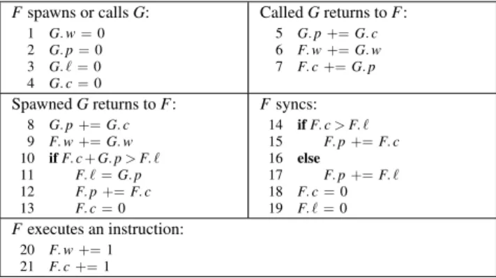
• The continuation F. c stores the span of the trace from the con-tinuation of u through the most recently executed instruction in F. Fspawns or calls G: 1 G. w = 0 2 G. p = 0 3 G. ` = 0 4 G. c = 0 Called G returns to F: 5 G. p += G. c 6 F. w += G. w 7 F. c += G. p Spawned G returns to F: 8 G. p += G. c 9 F. w += G. w 10 if F. c + G. p > F. ` 11 F. ` = G. p 12 F. p += F. c 13 F. c = 0 Fsyncs: 14 if F. c > F. ` 15 F. p += F. c 16 else 17 F. p += F. ` 18 F. c = 0 19 F. ` = 0 Fexecutes an instruction: 20 F. w += 1 21 F. c += 1

Figure 3: Pseudocode for Cilkprof’s work-span algorithm. For simplicity, this pseudocode computes work and span by incrementing the work and continuation at each instruction, rather than by any of several more efficient methods to compute instruction counts.

The work-span algorithm

Figure 3 gives the pseudocode for the basic Cilkprof algorithm for computing work and span. At any given moment during Cilkprof’s serial execution of the program under test, each nonzero work-span variable z holds a value corresponding to a trace, which we define as the trace of the value and denote by Trace(z). The pseudocode maintains three invariants:

INVARIANT1. The trace of the value in a variable is well

de-fined, that is, it is a contiguous subsequence of XI.

INVARIANT2. If z is a work variable, then z = Work(Trace(z)).

INVARIANT3. If z is a span variable, then z = Span(Trace(z)).

These invariants can be verified by induction on instruction count by inspecting the pseudocode in Figure 3. For example, just before Greturns from a spawn, we can assume inductively that G. p and G. c hold the spans of their traces. At this point, the trace of G. p starts at the first instruction of G and ends with u, traversing all called and spawned children in between. The trace of G. c starts at the continuation of u and continues to the current instruction, also traversing all called and spawned children in between. Thus, they have explored the entire trace of G between them. Consequently, when line 8 executes, the trace of G. p becomes the entire trace of G, and G. p becomes Span(()G. p, maintaining the invariants. Other code sequences succumb to similar reasoning.

Performance

The next theorem bounds the running time and space usage of Cilkprof’s algorithm for computing work and span.

(6)

LEMMA4. Cilkprof computes the work and span of a Cilk com-putation in O(T1) time using O(D) space, where T1is the work of the Cilk computation and D is the maximum call-stack depth of the computation.

PROOF. Inspection of the pseudocode from Figure 3 reveals that a constant number of operations on work-span variables occur at each function call or spawn, each sync, and each function return in the computation. Consequently, the running time is O(T1). Since there are 4 work-span variables in each frame of the shadow stack, the space is O(D).

4. THE BASIC PROFILE ALGORITHM

This section describes the basic algorithm that Cilkprof uses to compute profiles for a Cilk computation. We first introduce the ab-stract interface for the prof data structure, whose implementation is detailed in Section 5. We show how to augment the work-span algorithm to additionally compute profiles for the computation. We analyze Cilkprof under the assumption, borne out in Section 5, that the prof data structure supports all of its methods in Θ(1) amor-tized time. We show that Cilkprof executes a Cilk computation in O(T1) time, where T1is the work of the original Cilk computation.

The prof data structure

As it computes the work and span of a Cilk computation, Cilkprof updates profiles in a prof data structure, which records work and span data for each call site in the computation. Let us see how Cilkprof computes these profiles, in terms of the abstract interface to the prof data structure. Section 5 describes how a prof can be implemented efficiently.

The prof data structure is a key-value store R that maintains a set of key-value pairs hs, vi as elements, where the key s is a call site and the value v is a record containing a work field v. work and a span field v. span. The following methods operate on prof’s: • INIT(R): Initialize prof R to be an empty profile, deleting any

key-value pairs stored in R.

• UPDATE(R, hs, vi): If no element hs, v0i already exists in R, store

hs, vi into R. If such an element exists, store hs, v0_{+ vi, where} corresponding fields of v0and v are summed.

• ASSIGN(R, R0): Move the contents of prof R0into R, deleting

any old values in R, and then initialize R0.

• UNION(R, R0): Update the prof R with all the elements in the profR0, and then initialize R0.

• PRINT(R): List all the key-value pairs in the prof R, and initial-ize R.

We shall show in Section 5 that each of these methods can be im-plemented to execute in Θ(1) amortized time.

Profiles

What profiling data does Cilkprof compute? Consider a call site s. During a serial execution of the program, the function ϕ(s) con-taining s may call or spawn a function (or functions, if the target of the call or spawn is a function pointer) at s. Let OW be the set of executed call sites for which xi ∈ OW implies that σ (xi) = s. For each xi ∈ OW, recall that Trace(xi) is the set of instructions exe-cuted after the call or spawn at the call site until the corresponding return. Intuitively, the work-on-work for s is the total work of all of these calls, which is to say

X

xi∈OW

Work(Trace(xi)) , and the span-on-work for s is

X

xi∈OW

Span(Trace(xi)) .

The work-on-span and span-on-span for s are similar, where the sum is taken over OS, the set of instructions along the span of the computation for which xi ∈ OS implies that ϕ(xi) = s. These def-initions are inadequate, however, for recursive codes, because two instantiations of s on the call stack cause double counting. Rather than complicate the explanation of the algorithm at this point, let us defer the issue of recursion until Section 6 and assume for the remainder of this section that no recursive calls occur in the execu-tion, in which case these profile values for s are accurate.

Cilkprof computes these profile values for all call sites in the program by associating a prof data structure with each work-span variable in Figure 3. For a variable z, let z. prof denote z’s prof, let z. prof [s]. work denote the value of the work field for a call site s ∈ I in the profile data for z, and let z. prof [s]. span denote the value of z. prof ’s span field for s.

The Cilkprof algorithm

As Cilkprof performs the algorithm in Figure 3, in addition to com-puting the work and span, it also updates the prof associated with each work-span variable. First, just before each of lines 6 and 9, Cilkprof executes

UPDATE(G. w. prof , hs, [work : G. w, span : G. p]i)

UPDATE(G. p. prof , hs, [work : G. w, span : G. p]i) .

In addition, Cilkprof performs the following calculations, where y and z denote two distinct variables in the pseudocode:

• Whenever the pseudocode assigns y = 0, Cilkprof also executes INIT(y. prof ).

• Whenever the pseudocode assigns y = z, Cilkprof also executes

ASSIGN(y. prof , z. prof ).

• Whenever the pseudocode executes y += z, Cilkprof also exe-cutes UNION(y. prof , z. prof ).

As a point of clarification, executing lines 20–21 causes no addi-tional calculations to be performed on prof data structures, because 1 is not a variable.

Correctness

Recall that each work-span variable z in Figure 3 defines a trace Trace(z). For each variable z and call site s ∈ I, Cilkprof maintains the invariant

z. prof [s]. work = X xi∈Trace(z):σ (xi)=s

Work(Trace(xi))

and a similar invariant for z. prof [s]. span. One can verify by in-duction on instruction count that the Cilkprof algorithm maintains these invariants.

Analysis of performance

The next theorem bounds the running time and space usage of Cilkprof. This analysis assumes that all prof methods execute in Θ(1) amortized time and that a single prof occupies O(S) space, where S is the number of call sites in the Cilk computation. Sec-tion 5 shows how prof can achieve these bounds.

THEOREM5. Cilkprof executes a Cilk computation in O(T1)

time using O(DS) space, where T1 is the work of the Cilk com-putation, D is the maximum stack depth of the comcom-putation, and S is the number of call sites in the computation.

PROOF. By Lemma 4, the work-span algorithm contributes neg-ligibly to either time or space, and so it suffice to analyze the contri-butions due to method calls on the prof data structure. Inspection of the pseudocode from Figure 3, together with the modifications to make it handle profiles, reveals that a constant number of operations

(7)

on work-span variables occur at each function call or spawn, each sync, and each function return in the computation. Returning from a function causes a constant number of method calls on the prof to be performed, and each operation on a variable induces at most a constant number of method calls on its associated prof, each of which takes Θ(1) amortized time, as Theorem 6 in Section 5 will show. Consequently, each operation performed by Cilkprof to com-pute the work and span incurs at most constant overhead, yielding O(T1) for the total running time of Cilkprof.

The space bound is the product of the maximum depth D of func-tion nesting and the maximum size of a frame on the shadow stack. Each frame of the shadow stack contains 4 work-span variables and their associated prof data structures, each of which has size at most S. Thus, since the size of a frame on the shadow stack is O(S), the total space is O(DS).

5. THE PROF DATA STRUCTURE

This section describes how the the prof data structure employed by Cilkprof is implemented. We first assume that the number of call sites is known a priori. We investigate the problems that arise when implementing a prof as an array or linked list, and then we see how a hybrid implementation can achieve Θ(1) amortized time for all its methods. We then remove the assumption and extend profto the situation when call sites are discovered dynamically on the fly while still maintaining a Θ(1) amortized time1 for each of its methods.

The basic data structure

To simplify the description of the implementation of the prof data structure, assume for the moment that Cilkprof magically knows a priorithe number S of call sites in the computation. The compiler sets up a global hash table h mapping each call site s to a distinct index h(s) ∈ {0, 1, . . . , S − 1}.

The prof data structure is a hybrid of two straightforward im-plementations: an array and a list. Separately, each implementation would use too much time or space, but in combination they yield the desired space and time.

The array implementation represents a prof R as a size-S array R. arr[0 . . S − 1]. In this implementation, the INITmethod allocates a new size-S array R. arr and zeroes it, costing Θ(S) time. The call

UPDATE(R, hs, vi) updates the entry with R. arr[h(s)] + v (where

+ performs fieldwise addition on the work and span fields of the records), taking only Θ(1) time. UNION(R, R0) iterates through the entries of R0 and updates the corresponding entries in R, zeroing R0as it goes, costing Θ(S) time. Finally, ASSIGN(R, R0) iterates through the arrays copying the elements of R0to R, zeroing R0as it goes, also costing Θ(S) time. The inefficiency in the array imple-mentation is due to the Θ(S)-time methods.

The list implementation represents a prof R as a linked list R. `` that logs updates to the elements stored in R. The linked list R. `` is a singly linked list with a head and a tail pointer to support Θ(1)-time concatenation. The INIT, UPDATE, and UNION functions are implemented using straightforward Θ(1)-time linked list oper-ations. The INITmethod first deallocates any previous linked list, freeing the entries of R. `` in Θ(1) amortized time, because each en-try it frees must have been previously appended by UPDATE. Then INITallocates an empty linked list withNULLhead and tail point-ers. Calling UPDATE(R, hs, vi) appends a new linked-list element to R. `` containing hs, vi. Performing UNION(R, R0) concatenates the linked lists R. `` and R0. ``, and sets R0. `` to an empty linked list.

1_{Technically, the bound is Θ(1) expected time, because the implementation}

uses a hash table, but except for this one nit, the amortized bound better characterizes the performance of the data structure.

INIT(R) 1 Free R. arr 2 Free R. `` 3 R. `` = /0 4 R. arr = /0 ASSIGN(R, R0₎ 5 INIT(R) 6 R. `` = R0_{. ``} 7 R. arr = R. arr 8 R0. `` = /0 9 R0. arr = /0 _FLUSHLIST(R) 10 if R. arr == /0

11 R. arr = new Array(S)

12 for hs, vi ∈ R. `` 13 R. arr[h(s)] += v 14 Free R. `` UPDATE(R, hs, vi) 15 if R. arr , /0 16 R. arr[h(s)] += v

17 else APPEND(R. ``, hs, vi)

18 if |R. ``| == S 19 _FLUSHLIST(R) UNION(R, R0₎ 20 if R. arr , /0 21 if R0_{. arr , /0} 22 for i = 0 to S − 1 23 R. arr[i] += R0_{. arr[i]} 24 Free R0_{. arr}

25 else R. arr = R0_{. arr}

26 CONCATENATE(R. ``, R0_{. ``)} 27 if |R. ``| ≥ S 28 _FLUSHLIST(R) 29 R0_{. arr = /0} 30 R0. ll = /0 PRINT(R) 31 _FLUSHLIST(R) 32 for i = 0 to S − 1 33 Output R. arr[i] 34 INIT(R)

Figure 4: Pseudocode for the methods of the prof data structure, including a helper routine _FLUSHLIST. A prof R consists of a linked-list component R. `` and an array component R. arr. The linked list R. `` is a singly linked list with a cardinality field to keep track of the number of elements in the list and a head and tail pointer to enable Θ(1)-time list concatenation.

Similarly, PRINToperates in Θ(1) amortized time. The inefficiency in this implementation is space. Because every call to UPDATE al-locates space for an update, the linked list uses space proportional to the total number of updates, which, for a Cilk computation with work T1, is Θ(T1) space.

The hybrid implementation that Cilkprof actually uses repre-sents a prof R using both an array R. arr and a linked list R. ``. Figure 4 gives the pseudocode for the prof methods. Conceptually,

UPDATEand UNIONuse the linked list R. `` to handle elements

un-til R. `` contains at least S updates. At this point, the elements in R. `` are updated into the array R. arr, the linked list R. `` is emp-tied, and UPDATEand UNIONuse the array R. arr to handle future operations.

Intuitively, by combining the linked-list and array implementa-tions, the prof data structure R enjoys the time efficiency of the linked list implementation with the space efficiency of the array im-plementation. Because UPDATEand UNIONmove elements from R. `` into R. arr when R. `` contains at least S elements, R occupies O(S) space. By initially storing elements in a linked list, the prof data structure can avoid performing an expensive UNIONoperation until it can amortize that expense against the elements that have been inserted. The following theorem formalizes this intuition.

THEOREM6. The prof data structure uses at most Θ(S) space

and supports each of INIT,ASSIGN,UPDATE,UNION, andPRINT in Θ(1) amortized time.

PROOF. The time bound follows from an amortized analysis carried out using the accounting method [8, Ch. 17]. The amor-tization maintains the following invariants.

INVARIANT7. Each linked-list element carries 2 tokens of

amortized time.

INVARIANT8. Each array A carries |A| tokens of amortized

time.

(8)

A call to INIT(R) takes Θ(1) time to free R. arr and spends 1 token on each element in R. `` to cover the cost of freeing that el-ement. Then INITperforms Θ(1) operations in Θ(1) time to reini-tialize the data structure, for a total of Θ(1) amortized time.

A call to ASSIGNis Θ(1) time plus a call to INIT, for a total amortized time of Θ(1).

The helper routine _FLUSHLIST(R) is called only when its linked list R. `` attains at least S elements. The routine may spend Θ(S) time to create a new array of size S, the entries of which are initialized to 0. This routine can use 1 token from each ele-ment in R. `` to transfer that eleele-ment’s update to R. arr, free that element, transfer the element’s other token to R. arr, and cover the Θ(1) real cost to initialize one entry of R. arr. Consequently, _FLUSHLIST takes Θ(1) amortized time and produces an array R. arr with |R. ``| ≥ S = |R. arr| tokens, maintaining Invariant 8.

A call to UPDATE(R, hs, vi) exhibits one of three behaviors. First, if the call executes line 16, then it takes Θ(1) real time. Otherwise, the call executes line 17, which is charged Θ(1) real time plus 2 amortized time units to append a new linked-list element with 2 tokens onto R. `` while maintaining Invariant 7. At this point, if |R. ``| = S, then line 19 calls _FLUSHLIST, which costs Θ(1) amor-tized time. Thus, UPDATEtakes Θ(1) amortized time in every case. A call to UNION(R, R0) uses the tokens on R0. arr to achieve a Θ(1) amortized running time. If the call executes lines 22–24, then each iteration charges 1 token from R0. arr to cover the Θ(1) real cost to update an entry in R. arr with an entry in R0. arr. Lines 22–24 therefore take Θ(1) amortized time. Line 26 takes Θ(1) time to concatenate two linked lists, and the analysis of lines 27–30 corresponds to that for lines 18–19 of UPDATE. The amortized cost of UNIONis therefore Θ(1).

A call to PRINT(R) executes _FLUSHLIST in line 31 in Θ(1) amortized time, and spend the S available tokens in R. arr to pay for sequencing through all the elements of R. Adding in the cost to call INITin line 34 gives Θ(1) total amortized cost of printing.

The space bound on a prof data structure R follows from ob-serving that the array R. arr occupies Θ(S) space, and only line 17

in UPDATEand line 26 in UNIONincrease the size of the linked-list

R. `. Because lines 18–19 in UPDATEand lines 27–30 in UNION move the elements of R. `` into R. arr once the size of R. `` is at least S, the linked list R. `` never contains more than 2S elements, and R therefore occupies O(S) total space.

Discovering call sites dynamically

Let us now remove the assumption that the number S of call sites is known a priori. To handle call sites discovered dynamically as the execution unfolds, Cilkprof tracks the number S of unique call sites encountered so far. Cilkprof maintains the global hash table h using table doubling [8, Sec. 17.4], which can resize the table as it grows while still providing amortized Θ(1) operations. When Cilkprof encounters a new call site s, it increments S and stores h(s) = S − 1, thereby mapping the new call site to the new value of S − 1.

We must also modify the helper function _FLUSHLIST. First, line 15 must check whether the size of the existing array matches the current value of S, rather than simply checking if it exists. If a new array is allocated, in addition to the linked-list elements being transferred to the new array, the old array elements must also be transferred. At the end, the old array must be destroyed.

We must also modify the UPDATEand UNIONmethods to en-sure that both UPDATEand UNIONmaintain the same invariants in their amortization as stated in the proof of Theorem 6. Thus, the changes do not affect the asymptotic complexity of the prof data structure. Specifically, line 15 in the pseudocode for UPDATEmust be modified as in _FLUSHLIST to check whether the size of the

1 int fib ( int n ) {

2 if ( n < 2) r e t u r n n ; 3 int x , y ; 4 x = c i l k _ s p a w n fib ( n -1) ; 5 y = fib (n -2) ; 6 c i l k _ s y n c ; 7 r e t u r n ( x + y ) ; 8 }

11 int n , r e s u l t ;

12 // par se a r g u m e n t s

13 r e s u l t = fib ( n ) ;

14 r e t u r n 0;

15 }

Figure 5: Cilk pseudocode for a recursive program to compute Fibonacci numbers. main() fib(4) 1 2 fib(3) fib(2) fib(1) fib(1) fib(0) fib(2) fib(1) fib(0) 1 1 1 2 2 2

Figure 6: An invocation tree for the recursive Fibonacci program in Fig-ure 5. Each rounded rectangle denotes a function instantiation, and an edge between tow rounded rectangles denotes the upper instantiation invoking the lower. The circled labels 1 and 2 on edges identify the call sites on lines 4 and 5, respectively, in the code in Figure 5.

existing array matches the current value of S. With this change, a call to UPDATEadds a record to the linked list whenever the array is too small, even if the array already stores some records. Lines 20–25 in the pseudocode for UNIONmust also be modified to copy the elements of the smaller array into the larger.

6. THE PROFILE

This section describes the profile that Cilkprof computes. Al-though Section 4 describes how Cilkprof can measure the work and span of each call site assuming the program contains no recursive functions, in fact, Cilkprof must handle recursive functions with care to avoid overcounting their work and span. We define the “top-call-site,” “top-caller,” and “local” measurements that Cilkprof ac-cumulates for each call site, each of which we found to be easy to compute and useful for analyzing the contribution of that call site to the work and span of the overall program. We describe how to compute these measures.

A Cilkprof measurement for a call site s consists of the follow-ing values for a set of invocations of s:

• an execution count — the number of invocations of s accumu-lated in the profile;

• the call-site work — the sum of the work of those invocations; • the call-site span — the sum of the spans of those invocations. Cilkprof additionally computes the parallelism of s as the ratio of s’s call-site work and call-site span.

(9)

If programs contained no recursive functions, Cilkprof could simply aggregate all executions of each call site, but generally, it must avoid overcounting the call-site work and call-site span of recursive functions. Of the many ways that Cilkprof might accom-modate recursive functions, we have found three sets of measure-ments of a call site, called the “top-call-site,” “top-caller,” and “lo-cal” measurements, to be particularly useful for analyzing the par-allelism of Cilk computations. These measurements maintain the basic algorithm’s performance bounds given in Theorems 5 and 6 while also handling recursion.

Top-call-site measurements

Conceptually, the “top-call-site” measurement for a call site s ag-gregates the work and span of every execution of s that is not a recursive execution of s. Formally, an executed call site xs ∈ I is a top-call-site invocation if no executed call site xi ∈ I exists such that

xs∈ Trace(xi) ∧ σ (xs) = σ (xi) .

Cilkprof’s site measurement for s aggregates all top-call-site invocations of s.

An executed call site can be identified as a top-call-site invoca-tion from the computainvoca-tion’s invocainvoca-tion tree. Consider the example invocation tree in Figure 6 for the parallel recursive Cilk program in Figure 5. Each edge in this tree corresponds to an invocation — an executed call site that either calls or spawns a child — and the labels on edges denote the corresponding call site. From Figure 6, we see that the executed call site spawning fib(3) is a top-call-site invocation, because no other execution of line 4 appears above fib(3)in the invocation tree. The spawning of fib(2) by fib(3) is not a top-call-site invocation, however, because fib(3) appears above fib(2) in the tree.

Cilkprof’s top-call-site measurements are useful for assessing the parallelism of each call site. The ratio of the call-site work over the call-site span from a call site’s top-call-site data gives the parallelism of all nonrecursive executions of that call site in the computation, as if the computation performed each such call site execution in series. This parallelism value can be particularly help-ful for measuring the parallelism of executed call sites that occur on the critical path of the computation.

In a function containing multiple recursive calls, however, such as the fib routine in Figure 5, the top-call-site measurements are less useful for comparing different call sites’ relative contributions. For example, consider the top-call-site work and span values in Fig-ure 7, which Cilkprof collected from running the code in FigFig-ure 5. As Figure 7 shows, the top-call-site work values for the recursive fibinvocations on line 4 and line 5 are similar to that of the call to fibon line 13, and the top-call-site span values of these recursive invocations exceed that of line 13.

These large top-call-site measurements occur because the mea-surement aggregates multiple top-call-site executions of a call site under the same top-level call to fib. For example, as the invoca-tion tree in Figure 6 shows, the invocainvoca-tions of fib(1) from fib(3), fib(2)from fib(4), and fib(0) from fib(2) under fib(3) are all top-call-site invocations for line 5. Similarly, the invocations of fib(3)from fib(4) and of fib(1) from fib(2) under fib(4) are both top-call-site invocations for line 4.

Top-caller measurements

In contrast to top-call-site measurements, the “top-caller” measure-ment for a call site s conceptually aggregates the work and span of every execution of s from a nonrecursive invocation of its caller. Formally, an executed call site xs ∈ I is a top-caller invocation if

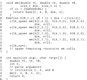
1 void mm ( d o u b l e *C , d o u b l e * A , d o u b l e * B , 2 s i z e _ t dim , s i z e _ t n ) { 3 if ( n < C O A R S E N I N G ) { 4 r e t u r n base ( C , A , B , dim , n ) ; 5 } 6 # d e f i n e X (M ,r , c ) ( M + ( r * dim + c ) *( n /2) ) 7 c i l k _ s p a w n mm ( X ( C ,0 ,0) , X ( A ,0 ,0) , X ( B ,0 ,0) , 8 dim , n /2) ; 9 c i l k _ s p a w n mm ( X ( C ,0 ,1) , X ( A ,0 ,0) , X ( B ,0 ,1) , 10 dim , n /2) ; 11 c i l k _ s p a w n mm ( X ( C ,1 ,0) , X ( A ,1 ,0) , X ( B ,0 ,0) , 12 dim , n /2) ; 13 mm ( X ( C ,1 ,1) , X ( A ,1 ,0) , X ( B ,0 ,1) , 14 dim , n /2) ; 15 c i l k _ s y n c ; 16 // spa wn r e m a i n i n g r e c u r s i v e mm ca lls 17 }

20 d o u b l e * C , * A , * B ; 21 int n ; 22 // par se a r g u m e n t s 23 // i n i t i a l i z e C , A , and B 24 mm ( C , A , B , n , n ) ; 25 r e t u r n 0; 26 }

Figure 8: Cilk pseudocode for a divide-and-conquer parallel matrix-multiplication program. The recursive mm routine in this program calls the function base in its base case. The variable COARSENING is a fixed constant defining the maximum size of matrices to multiply in the base case.

no executed call site xi ∈ I exists such that

xs∈ Trace(xi) ∧ ϕ(σ (xs)) = ϕ(σ (xi)) .

Cilkprof’s top-caller measurement for a call site s aggregates all top-caller invocations of s.

Like top-call-site invocations, top-caller invocations can be iden-tified from the computation’s invocation tree. Once again, consider the code in Figure 5 and its example invocation tree in Figure 6. The invocation producing fib(3) is a top-caller invocation, be-cause no instantiation of fib exists above fib(4), the function in-stantiation containing this invocation, in the tree. The invocation producing fib(1) under the right child of fib(4) is not a top-caller invocation, however, because fib(4) is an instantiation of fibabove the instantiation fib(2) that contains this invocation. The top-caller invocations that occur in the invocation tree in Fig-ure 6, therefore, are from main() to fib(4) and from fib(4) to each of its children.

Top-caller measurements can be useful for comparing call sites in the same function. The top-caller measurements in Figure 7, for example, show that the ratio of the aggregate work of the top-caller invocations of lines 4 and 5 is 279, 094, 680/171, 229, 726 ≈ 1.63, which is approximately the golden ratio φ = (1 +√5)/2 ≈ 1.61. This relationship makes sense, because fib(n) theoretically incurs Θ(φn) work.

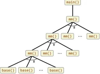
The top-caller measurements provide no information for call sites that are never reached from a top-level instantiation of a function, however. Consider the divide-and-conquer matrix-multiplication program in Figure 8 and its invocation tree illustrated in Figure 9. As Figure 9 shows, the function base called in the base case of mm is never called by the top-caller invocation of mm from main. Consequently, as the top-caller measurements in Figure 10 for this program show, Cilkprof measures the top-caller call-site work and span values for base to be 0. From these top-caller val-ues, one cannot conclude that most of the computation of mm, in fact, occurs under calls to base.

Local measurements

The local measurement for a call site aggregates a “local work” and a “local span” for every execution of that call site. The local work of an executed call site xs ∈ I is the work in Trace(xs) minus

(10)

Top-call-site Top-caller Local

Line T1 T∞ T1/T∞ T1 T∞ T1/T∞ T1 T∞ T1/T∞

4 450, 321, 639 113, 267 3, 975.8 279, 094, 680 39, 643 7, 040.2 150, 281, 850 150, 281, 850 1.0 5 450, 307, 915 250, 302 1, 799.1 171, 229, 726 14, 688 11, 657.8 121, 330, 045 86, 699, 953 1.4 13 450, 325, 186 40, 331 11, 165.7 450, 325, 186 40, 331 11, 165.7 780 688 1.1

Figure 7: Work and span values in the on-work profile Cilkprof collects for running the recursive Fibonacci program in Figure 5 to compute fib(30). All times are measured in nanoseconds.

Top-call-site Top-caller Local

Line T1 T∞ T1/T∞ T1 T∞ T1/T∞ T1 T∞ T1/T∞ 4 185, 830, 187 185, 830, 187 1.0 0 0 — 185, 830, 187 185, 830, 187 1.0 7 77, 417, 401 22, 010, 873 3.5 23, 473, 633 405, 947 57.8 195, 079 177, 786 1.1 9 77, 475, 639 21, 983, 150 3.5 23, 384, 174 411, 099 56.9 183, 232 168, 249 1.1 11 77, 440, 990 21, 988, 390 3.5 23, 403, 194 402, 281 58.2 187, 472 169, 541 1.1 13 77, 262, 499 21, 853, 710 3.5 23, 378, 967 387, 880 60.3 110, 374 97, 656 1.1 24 187, 150, 784 803, 122 233.0 187, 150, 784 803, 122 233.0 1, 563 957 1.6

Figure 10: Work and span values in the on-work profile Cilkprof produces for running the divide-and-conquer matrix multiplication code in Figure 8 to multiply two 512 × 512 matrices of doubles. All times are measured in nanoseconds.

main() mm() mm() base() base() mm() mm() base()

⋯

mm() mm()

⋯

mm()

⋯

8 8 8

Figure 9: An invocation tree for the matrix-multiplication program in Fig-ure 8. Each rectangle denotes a function instantiation, and an edge from one rectangle to a rectangle below it denotes the upper invocation calling the lower.

the work in the traces of the functions that xs invokes. By ignor-ing the contributions of its children, the local work and local span values for all executions of a call site can be aggregated without overcounting executed instructions in recursive calls.

The local measurements call sites are often useful for examining functions invoked in the base case of a recursive routine. The local measurements for mm in Figure 10, for example, make it clear that most of the total work of the call to mm from main occurs in calls to base. Furthermore, as we observed in the quicksort example in Section 2, these local work and span values can effectively identify which functions contribute directly to the span of the computation. The local parallelism of a call site s — the ratio of the local work and local span of s — does not accurately reflect the parallelism of s, however. As Figure 10 shows, by excluding the work and span contributions of each executed call site’s children, most local-parallelism values are close to 1, even for call sites such as line 24 which exhibit ample parallelism.

The top-call-site, top-caller, and local measurements for a call site s each measure qualitatively different things about s. Each of these measurements seems to be useful for analyzing a parallel pro-gram in different ways. An interesting open question is whether

there are other measurements that are as useful as these three for diagnosing scalability bottlenecks.

7. EMPIRICAL EVALUATION

To implement Cilkprof, we modified a branch [19] of the LLVM [26] compiler that supports Cilk Plus [16] to instrument function entries and exits, as well as calls into the Cilk runtime from the program to handle cilk_spawn and cilk_sync statements. A Cilk program is compiled with the modified compiler produces a binary executable that executes the Cilkprof algorithm as a shadow com-putation. On a suite of 16 benchmark programs, we compared the Cilkprof running time of each benchmark with the benchmark’s se-rial running time compiled with the unmodified compiler, both exe-cutions using optimization level -O3. Compared with this “native” serial execution, Cilkprof incurs a geometric-mean multiplicative slowdown of 1.9 and a maximum slowdown of 7.4.

Results

We compared the running time of Cilkprof on each benchmark to the native serial running time of the benchmark, that is, the running time of the benchmark when compiled with no instrumentation. We ran our experiments on a dual-socket Intel Xeon E5-2665 system 2.4 GHz 8-core CPU’s having a total of 32 GiB of memory. Each processor core has a 32 KiB private L1-data-cache and a 256 KiB private L2-cache. The 8 cores on each chip share the same 20 MiB L3-cache. The machine was running Fedora 16, using a custom Linux kernel 3.6.11.

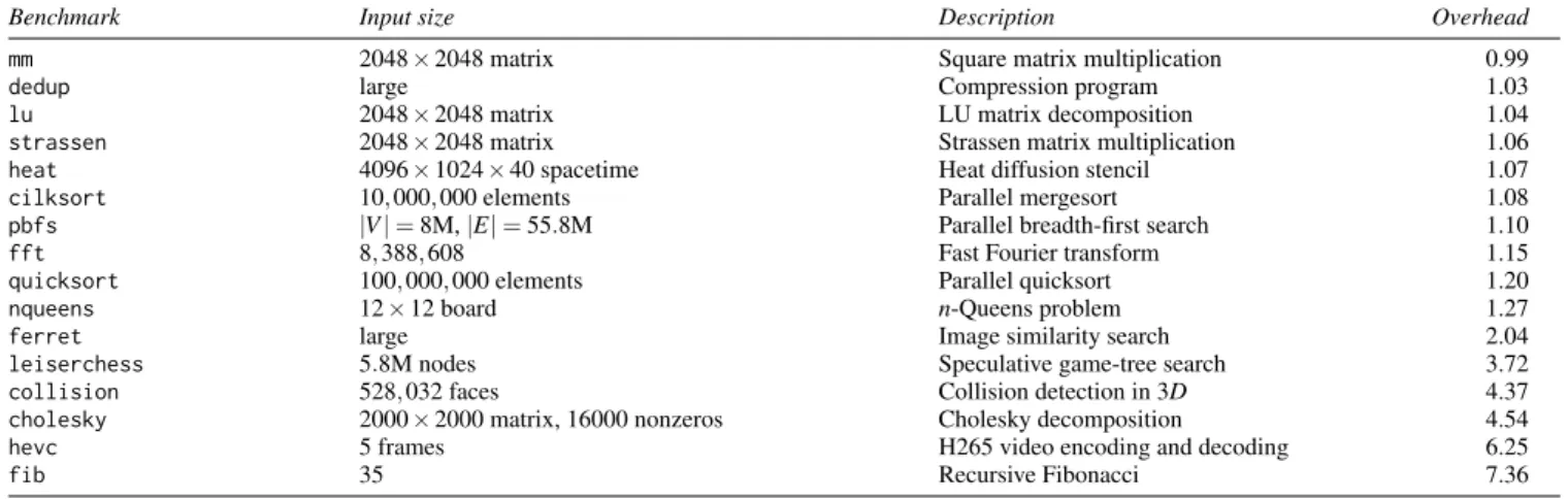
To study the empirical overhead of Cilkprof, we compiled a suite of 16 application benchmarks, as Figure 11 describes. The mm, quicksort, and fib benchmarks correspond to the Cilk pseu-docode in Figures 8, 1, and 5, respectively. The pbfs benchmark is a parallel breadth-first search code that implements the PBFS al-gorithm of [28]. We converted the dedup and ferret benchmarks from the PARSEC benchmark [3, 4] to use Cilk linguistics and a reducer_ostream(which is part of Cilk Plus) for writing output. The leiserchess program performs a parallel speculative game-tree search using Cilk. The hevc benchmark is a 30, 000-line im-plementation of the H265 video encoder and decoder [22] that we parallelized using Cilk. The remaining benchmarks are the same benchmarks included in the Cilk-5 distribution [10].

Figure 11 presents our empirical results. As the figure shows, the Cilkprof implementation incurs a geometric mean slowdown of 1.9× on these benchmarks compared to the uninstrumented

(11)

ver-sion of the benchmark. Furthermore, the maximum multiplicative overhead we observed on any benchmark was 7.4.

Optimizations

The implementation contains several optimizations:

• For basic timing measurements, we chose to use a cycle counter to measure blocks of instructions, rather than naively increment-ing a counter for every instruction executed, as in the basic pseu-docode from Figure 3. (We also adjust the measured numbers to compensate for the time it takes Cilkprof to execute the instru-mentation.)

• For a function F with no cilk_spawn’s, the implementation maintains only the prefix span variable F. p to store the span of F, rather than all 3 span variables.

• If a function G calls F, then the implementation sets the prof data structure for F. p to be the prof data structure for either G. p, if G has no outstanding spawned children when it calls F, or G. c, otherwise.

• When the span variable associated with a prof data structure R is set to 0, the implementation simply clears the nonempty entries of the array R. arr, rather than freeing its memory.

• The implementation maintains the set of nonempty entries in each prof data structure array in order to optimize the processes of combining and clearing those entries.

These optimizations reduced Cilkprof’s overhead on the fib benchmark by a factor of 5 and its overhead on the leiserchess benchmark dropped by a factor of 9.

At the risk of losing some information, Cilkprof declines to in-strument inlined functions, which, in Intel Cilk Plus, cannot spawn. To do so, we modified LLVM such that, when it inlines a function, it removes the instrumentation for the inlined version of that func-tion. When this program runs with Cilkprof, therefore, the work of the inlined function influences the work and span of its parent, but it will not create a separate entry in the profile Cilkprof produces.

We feel that this optimization is reasonable because inlined func-tions are typically unlikely to be scalability bottlenecks on their own. For example, the compiler often inlines C++ object methods to extract or set fields of that object, which the programmer wrote to provide a convenient abstraction in the program code, but which the compiler can often implement with a handful of data movement in-structions in the caller. If Cilkprof instruments such a function, then Cilkprof incurs overheads to measure and record very few instruc-tions. The cost of instrumenting such functions therefore seems to outweigh the benefits to scalability analysis.

We examined Cilkprof’s overhead when inlined functions are in-strumented on the application benchmarks. For all benchmarks ex-cept lu, leiserchess, collision, and hevc, Cilkprof incurred less than 2 times the overhead it incurred when inlined functions in that benchmark were not instrumented. On the leiserchess and collisionbenchmarks, however, instrumenting inlined functions increased Cilkprof’s overhead by a factor of 8–10. Both of these benchmarks make extensive use of small functions that simply get or set fields of an object, which are particularly light weight when inlined. Although this optimization does not affect every bench-mark, it can dramatically improve Cilkprof’s performance on the benchmarks it does affect.

8. CASE STUDY: PBFS

One of our first successes with Cilkprof2came when diagnosing a parallelism bottleneck in PBFS, an 1800-line parallel

breadth-2_{Actually, the original case study used the (much slower) Cilkprof}

Pin-tool [18] we built in collaboration with Intel. Since the data from this early experiment have since been lost, we recreated the experiment with our LLVM-based Cilkprof implementation.

first search Cilk program [28]. After just 2 hours of work using Cilkprof, we were able to identify a parallelism bottleneck in the PBFS code. Fixing this bottleneck enhanced the parallelism of the code by a factor of about 5. This section presents our experience diagnosing a scalability bottleneck in the PBFS code. You should not need to understand either the PBFS algorithm or its implemen-tation to follow this case study.

After designing and building PBFS, we observed that the code failed to achieve linear speedup on 8 processors. For example, PBFS was achieving a parallel speedup of 4 − 5 on our Grid3D200 benchmark graph, a 7-point finite-difference mesh generated using the Matlab Mesh Partitioning and Graph Separator Toolbox [12], on which PBFS explored 8M vertices and 55.8M edges during a search of depth 598. A back-of-the-envelope calculation suggested that the measured parallelism of PBFS should be around 200 − 400, ample for 8 processors, if one follows the rule of thumb that a pro-gram should have at least 10 times more parallelism than the num-ber of processors for scheduling overhead to be negligible.

We suspected that the scalability of this PBFS code suffered from insufficient memory bandwidth on the machine. For exam-ple, when we artificially inflated the amount of computation that the code performed in the base case of its recursive helper func-tions, then the code did exhibit linear speedup. The problem with this test, however, is that it also increased the parallelism of the code. We ran Cilkview on the original PBFS code to ensure that insufficient parallelism was not the issue. Cilkview, however, re-ported that the parallelism of this PBFS code was merely 12, which is not ample parallelism for 8 processors.

We ran the PBFS code with Cilkprof and examined Cilkprof’s profiles. The on-work profile showed us that the call to pbfs — our parallel BFS routine — from main accounted for most of the work of the program, and that the parallelism of pbfs was small, just as Cilkview had found. To discover what methods contributed most to the span, we sorted Cilkprof’s data by decreasing local T∞ on span. Viewing the data from this perspective showed us that the following three methods contributed the most to the span of the program overall:

1. First was a call to parseBinaryFile, a serial function that parses the input graph.

2. Second was a call to the serial Graph constructor to create the internal data structure storing the graph from the input. 3. Third was a call to pbfs_proc_Node, a function that

pro-cesses a constant-sized array of graph vertices.

Although the top two entries were not called from pbfs, the third entry for pbfs_proc_Node was called in the base case of the re-cursive helper methods of pbfs. Comparing the local T∞ on span of pbfs_proc_Node to the top-caller T∞of bfs showed us that this method accounted for 66% of the span of bfs. Furthermore, the top-call-site parallelism values from Cilkprof showed us that all in-vocations pbfs_proc_Node were serial.

These data led us to look more closely at pbfs_proc_Node. We discovered that this method evaluates a constant-sized array of ver-tices in the graph. Because the input array has constant size, this method evaluated the contents of this array serially. In the code, however, the size of this array was tuned to optimize the insertion of vertices into the array. The constant size of this array was there-fore too large for pbfs_proc_Node, causing the serial execution of pbfs_proc_Nodeto become a scalability bottleneck.

We parallelized the pbfs_proc_Node function to process its in-put array in parallel with an appropriate base-case size. We then ran our modified PBFS code through Cilkprof and sorted the new data by local T∞on span to examine the effect of our efforts. We found

(12)

Benchmark Input size Description Overhead

mm 2048 × 2048 matrix Square matrix multiplication 0.99

dedup large Compression program 1.03

lu 2048 × 2048 matrix LU matrix decomposition 1.04

strassen 2048 × 2048 matrix Strassen matrix multiplication 1.06 heat 4096 × 1024 × 40 spacetime Heat diffusion stencil 1.07

cilksort 10, 000, 000 elements Parallel mergesort 1.08

pbfs |V | = 8M, |E| = 55.8M Parallel breadth-first search 1.10

fft 8, 388, 608 Fast Fourier transform 1.15

quicksort 100, 000, 000 elements Parallel quicksort 1.20

nqueens 12 × 12 board n-Queens problem 1.27

ferret large Image similarity search 2.04

leiserchess 5.8M nodes Speculative game-tree search 3.72

collision 528, 032 faces Collision detection in 3D 4.37

cholesky 2000 × 2000 matrix, 16000 nonzeros Cholesky decomposition 4.54

hevc 5 frames H265 video encoding and decoding 6.25

fib 35 Recursive Fibonacci 7.36

Figure 11: Application benchmarks demonstrating the performance overhead of the Cilkprof prototype tool. The benchmarks are sorted in order of increasing overhead. For each benchmark, the Overhead column gives the ratio of its running time with when compiled with the Cilkprof implementation over its running time without instrumentation. Each ratio is computed as the geometric mean ratio of 5 runs with Cilkprof and 5 runs without Cilkprof. We used a modified version of the Cilk Plus/LLVM compiler to compile each benchmark with Cilkprof, and we used the original version of the Cilk Plus/LLVM compiler to compile the benchmarks with no instrumentation. The Cilkprof implementation and benchmark codes were compiled using the -O3 optimization level.

that, although pbfs_proc_Node was still the third-largest contribu-tor to the span of the program, the local T∞on span is a factor of 6 larger. Furthermore, the parallelism of pbfs is now 60, a factor of 5 larger than its previous value. Finally, pbfs_proc_Node accounts for 48% of this span. We also confirmed that reducing the new base-case size of pbfs_proc_Node can increase the parallelism of pbfsto 100, at the cost of scheduling overhead.

9. RELATED WORK

This section reviews related work on performance tools for par-allel programming.

We chose to implement Cilkprof using compiler instrumentation (e.g., [31, 32]), but there are other strategies we could have used to examine the behavior of a computation, such as asynchronous sam-pling (e.g., [13]) and binary instrumentation (e.g., [6, 9, 29, 30]). Although asynchronous sampling provides low-overhead solutions for some analytical tools, we do not know of a way to mea-sure the span of a multithreaded Cilk computation by sampling. Cilkview [14] is implemented using the Pin binary-instrumentation framework [29] augmented by support in the Intel Cilk Plus com-piler [20] for low-overhead annotations [17], and we collaborated with Intel to build a prototype Cilkprof as a Pintool. Because we found that this prototype Cilkprof ran slowly, we chose to imple-ment Cilkprof using compiler instruimple-mentation in order to improve its performance. In fact, because it uses compiler instrumentation, the Cilkprof implementation outperforms the existing Cilkview im-plementation, which only computes work and span for the entire computation and does not produce profiles of work and span for every call site as Cilkprof does.

Many parallel performance tools examine a parallel computation and report performance characteristics specific to that architecture and execution. Tools like HPCToolkit [1], Intel VTune Ampli-fier [21], and others [7,25,33] measure system counters and events, and provide reports based on a program execution. HPCToolkit, in particular, is an integrated suite of tools to measure and ana-lyze program performance that sets a high standard for capability and usability. HPCToolkit uses statistical sampling of timers and hardware performance counters to measure a program’s resource consumption, and attributes measurements to full calling contexts.

Other approaches for identifying scalability bottlenecks include normalized processor time [2] or the more precise parallel idleness metric [34]. The idea is that, in a work-stealing concurrency

plat-form, if at some particular point in time some worker threads are idle, then we can assign blame to the function that is running on the other workers: if that function were more parallel, then the idle threads would be doing something useful. These are helpful met-rics for identifying bottlenecks on the current architecture, and an-swer the question as to whether the program, run on a P-processor machine has at least P-fold parallelism. But they don’t provide scalability analysis beyond P processors.

In contrast to all of these applications and approaches, Cilkprof’s analysis applies to the measured work and span. Work and span are good metrics for inferring bounds on parallel speedup on ar-chitectures with any number of processors. A program compiled for Cilkprof will generate profile information that is generally ap-plicable, rather than just for the architecture on which it was run. Additionally, Cilkprof is distinguished in that it uses direct instru-mentation rather than statistical sampling.

Whereas Cilkprof computes the parallelism of call sites in a par-allel program, the Kremlin [11, 24] and Kismet [23] tools analyze serial programs to suggest parallelism opportunities and to predict the impact of parallelization. Kremlin can suggest which parts of a serial program might benefit from parallelization. It estimates the parallelism of a serial program using “hierarchical critical-path analysis” and connects to a “parallelism planner” to evaluate many possible parallelizations of the program. Based on its determina-tion of which regions (loops and funcdetermina-tions) of the program should be parallelized, it computes a work/span profile of the program, computing a “self-parallelism” metric for each region, which esti-mates the parallelism that can be obtained from parallelizing that region separate from other regions. The analysis produces a textual report as output suggesting which regions should be parallelized. Kismet, which is a product of the same research group, attempts to predict the actual speedup after parallelization, given a target ma-chine and runtime system.

10. CONCLUSION

Our work on Cilkprof has left us with some interesting research questions. We conclude by addressing issues of Cilkprof’s user interface, parallelizing Cilkprof, and making Cilkprof functionally more “complete.”

Chief among the open issues is user interface. How should the profiles produced by Cilkprof be communicated to a Cilk program-mer? Although we ourselves used just a spreadsheet to divine