HAL Id: inserm-00598351
https://www.hal.inserm.fr/inserm-00598351
Submitted on 6 Jun 2011HAL is a multi-disciplinary open access
archive for the deposit and dissemination of sci-entific research documents, whether they are pub-lished or not. The documents may come from
L’archive ouverte pluridisciplinaire HAL, est destinée au dépôt et à la diffusion de documents scientifiques de niveau recherche, publiés ou non, émanant des établissements d’enseignement et de
A multivolume visualization method for spatially aligned
volumes after 3D/3D image registration
Hui Tang, Jean-Louis Dillenseger, Xudong Bao, Limin Luo
To cite this version:
Hui Tang, Jean-Louis Dillenseger, Xudong Bao, Limin Luo. A multivolume visualization method for spatially aligned volumes after 3D/3D image registration. Innovation and Research in BioMedical en-gineering, Elsevier Masson, 2011, 32 (3), pp.195-203. �10.1016/j.irbm.2011.01.040�. �inserm-00598351�
A multi-volume visualization method for spatially
aligned volumes after 3D/3D image registration
M´ethode de fusion et de visualisation de volumes
spatialement align´es apr`es recalage 3D/3D
Tang Huia,b,c,d, Dillenseger Jean-Louisa,b,d, Bao Xu Dongc,d, Luo Liminc,d
aINSERM U642, 35042 Rennes, France
bUniversit´e de Rennes I, Laboratoire Traitement du Signal et de l’Image, 35042 Rennes,
France
cLaboratory of Image Science and Technology, Department of Computer Science and
Engineering, Southeast University, 210096, Nanjing, China
dCentre de Recherche en Information Biom´edicale Sino-Fran¸cais (CRIBs)
Abstract
Objective A new method for the visualization of spatially aligned volumes
after 3D/3D image registration is presented in this paper. This work aims at displaying the full information of the multi-volume in the same scene.
Materials and methods First, we form a vectorial volume from spatially
aligned multi-volume after 3D registration. Then, a statistical vectorial volume classification method based on neighborhood weighted Gaus-sian mixture model is applied to analyze the vectorial volume and get material distribution information. Finally, several rendering techniques are adapted to visualize the parameters.
Results We imply an application case: the visualization of preoperative
kidney planning system to express our visualization method, but this method is not limited to the specific application case.
Discussion According to the levels where the data intermixing occurs, our
method mixes the data at the earliest level so that it is called the acquisition level intermixing method.
R´esum´e
Objectifs Dans cet article nous pr´esentons une nouvelle m´ethode de visuali-sation de volumes de donn´ees align´ees apr`es recalage 3D/3D. L’objectif est de repr´esenter dans une mˆeme sc`ene l’ensemble de l’information align´ee.
Mat´eriel et m´ethodes Dans un premier temps, apr`es recalage, les donn´ees fusionn´ees dans un mˆeme rep`ere forment un volume de donn´ees vecto-rielles. Nous appliquons ensuite sur ce volume une m´ethode de classi-fication bas´ee sur une mixture de Gaussiennes pond´er´ees par une in-formation de voisinage. Cette classification nous permet d’estimer la r´epartition dans le volume des diff´erents tissus. Au final, diff´erentes techniques de visualisation 3D ont ´et´e adapt´ees pour pouvoir traiter le r´esultat de la classification.
R´esultats Notre technique a ´et´e valid´ee dans le cadre du planning pr´eop´eratoire d’une chirurgie r´enale par la visualisation des diff´erents tissus com-posant le rein. Notre m´ethode n’´etant pas limit´ee `a cette seule appli-cation, elle peut s’appliquer `a tous les cas pr´esentant un m´elange de donn´ees.
Discussion Contrairement aux m´ethodes de la litt´erature, notre technique travaille directement sur les donn´ees fusionn´ees. Elle peut donc ˆetre appel´ee ”m´ethode de visualisation par m´elange des donn´ees de d´epart”.
Keywords:
Direct volume rendering, Medical imaging, Multi-volume rendering, Scientific visualization, Vectorial volume classification, 3D image registration
Mots cl´es:
Classification de volumes vectoriels, Imagerie m´edicale, Recalage 3D, Rendu de volume, Visualisation de volumes fusionn´es, Visualisation scientifique
1. Introduction
In medical imaging, multiple images are often acquired from the same sub-ject at different times, and often with different imaging modalities. These
multiple acquisitions contain different kind of information of a complemen-tary nature (time evolution of metabolism, different anatomical structures, etc.). A medical image registration process must then be performed in order to bring the different acquisitions into a single reference space [1, 2, 3, 4, 5]. Image registration is the process of overlaying two or more images of the same scene at different times, from different viewpoints, and/or by different sensors [2]. After the 3D/3D registration, we got several volumes spatially-aligned on a common grid. If these volumes are rendered individually, the registration process will be useless. So that a combined presentation of reg-istered volume datasets is needed to give a better view of the information content, so that a multi-volume visualization method will be discussed in this paper.
For the visualization of a single volume, direct volume rendering convey an entire 3D dataset in a 2D image directly. Many studies have been conducted on direct volume rendering [6, 7, 8]. The process of constructing an image from a volumetric dataset using direct volume rendering can be summarized by the following steps [9]:
1. Data traversal: The positions of sample points within the volume are determined, which is usually according to the viewing point.
2. Sampling and interpolating: The dataset is sampled at the chosen po-sitions. The sampling points typically do not coincide with the grid points, and so interpolation is needed to recover the sample value. 3. Gradient computation: The data gradient is often needed, in particular
as an input to the shading component. Gradient computation requires additional sampling.
4. Transfer function: The sampled values are mapped to optical proper-ties, typically color and opacity values. The transfer function will help to visually distinguish materials in the volume.
5. Shading and illumination: Shading and illumination effects can be used to modulate the appearance of the samples. The three-dimensional impression is often enhanced by gradient-based shading which gives information about surface orientation.
6. Compositing: The pixels of the rendered image are computed by com-positing the optical properties and the colors of the sample points ac-cording to the volume rendering integral.
few literature did some research about multi-volume rendering techniques [10, 11, 12, 13].
The main idea of these multi-volume rendering algorithms is to mix the multi-information together at a certain level of the rendering pipeline. Cai and Sakas [10] classified the methods according to the levels where the data intermixing occurs. Three levels were defined: image level intermixing,
com-position level intermixing and illumination model level intermixing (Fig.1). • The simplest mixing technique is image level intermixing. It consists
to render each volume separately as a scalar dataset and then to blend the result images according to some weighting function that possibly includes the z-buffer of opacity channel. This method doesn’t require any modification of the volume renderer but it loses the depth ordering information.
• The composition level intermixing method solved this problem. For
each voxel of each volume, the opacity and color are estimated accord-ing to the voxel value and the illumination model. These opacities and colors are then intermixed at the compositing step, thus preserving the depth information. Most transfer function based methods belong to this category [12, 13].
• The third method is illumination model level intermixing. The volume
samples are combined before colors and opacities are computed. Cai and Sakas [10] proposed this method for their special application con-text and compared it with the two former methods. They also indicated its possibility to be applied in other multi-volume rendering contexts. All these above methods render the multi-volume by mixing the com-ponent volumes at one certain step of volume rendering pipeline. But ac-tually, these volumes are different acquisitions taken from the same patient so that they are not independent. While analyzing the registered volume dataset, each sample point should contain several elements which are sam-pled from the corresponding volumes. Therefore we can form a vectorial
volume dataset, in which each voxel contains a vector of n elements
corre-sponding to the information of the acquisitions (n is equal to the number of acquisitions). Then the analysis can be performed on this vectorial volume instead of several individual volumes. That is to say, the intermixing level can then occur before the rendering pipeline. We will call this level
first form a vectorial volume from the multi-volume; then apply a statistical multi-dimensional classification method to get the material property infor-mation; finally render the multi-volume according to the classified material properties.
The key idea of this paper is to consider the multi-volume as a vectorial volume and get the material distribution information by a vectorial volume classification method so that the acquisitions concerning the same subject can be considered together for the presentation of information. The rest of this paper is organized as follows. Section 2 expresses the proposed multi-volume rendering framework. The detail of the statistical vectorial multi-volume classification method is presented in section 3. After classification, several rendering methods can be used to display the material information, which are discussed in section 4. We take an application case of the proposed multi-volume visualization method for detail demonstration in this section. Finally, the conclusions are given in Section 5.
2. Multi-volume rendering framework
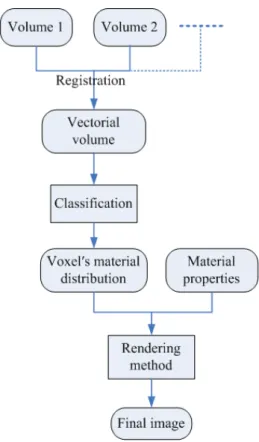
Based on the discussion in Section 1, we proposed a multi-volume render-ing method which belongs to the acquisition level intermixrender-ing. The frame-work of this method is described in Fig.2.
After registration, several volumes will be aligned into the same space (Fig.3-a to c). As analyzed before, the spatially aligned volumes can form a vectorial volume. If we analyze this vectorial volume instead of the individ-ual volumes, all acquisitions can be taken into account at the same time. So that we propose to first perform analysis on this vectorial volume and then apply rendering techniques to show the analysis result parameters. Since the multi-volumes are mixed together at the beginning, according to the lev-els where the data intermixing occurs, our method is called acquisition level
intermixing. The intermixing step is realized by a vectorial volume
classifi-cation method. It seems that any vectorial volume classificlassifi-cation technique can be applied in this framework. But see Fig.2 again, we can find that the rendering result relies much on the classification result so that the choice of the classification method becomes the essential step in this pipeline. We implemented a vectorial volume soft segmentation method based on neigh-borhood weighted Gaussian mixture model which has been presented in our previous paper [14] because this method is less affected by noises and it can avoid mis-classification on the boundaries.
After this classification, we get the material probability distributions on each grid of the volume. At this step, the user assigns some material prop-erties i.e. the material color Ck and the material global opacity αk with
1 ≤ k ≤ K, K the number of tissues (or material). With these material properties, several rendering techniques which are extended from scalar vol-ume rendering techniques can be applied to get the final image. For the rendering techniques for scalar volumes, most of the algorithms can be clas-sified into two categories: surface rendering algorithms and direct volume rendering algorithms [15]. Surface rendering algorithms first extract the sur-face representations from the volume data and then graphic techniques are used to render the extracted geometric primitives. Direct volume rendering algorithms get the final image from the volume data without going through an intermediate surface extraction step. In Section 4 we will show that both of the two rendering techniques can be adapted to the visualization of clas-sified vectorial volume.
3. Statistical vectorial volume classification
As mentioned in the introduction section, our initial data is a vectorial volume composed of I voxels denoted by xi (i = 1, 2, . . . , I) and where each
voxel is an n-dimensional vector (n the number of acquisitions). With K the number of tissues (or materials), the Gaussian mixture model assumes that each voxel is composed of K component densities mixed together with
K mixing coefficients. The kth component density is denoted by pk(xi|Θk)
governed by a parameter set Θk). Each component density follows a
Gaus-sian distribution with Θk the parameters of Gaussian, mean and standard
deviation. The kth mixing coefficient is denoted by βk. Based on statistical
theory, the parameters and mixing coefficients are estimated by maximum likelihood (ML) and expectation maximization (EM) algorithm is used as an optimization method so that we can get the class probabilities on each voxel according to the voxel intensity vector. But this model relies only on the intensity distributions, which will lead a misclassification on the boundaries and on inhomogeneous regions with noise. In order to solve this problem, we proposed a neighborhood weighted Gaussian mixture model by integrating the neighborhood information into the classification process according to the idea that for each voxel, the probability of the kth class should be affected by the neighbors’ kth class probabilities. This neighborhood information is integrated as a weight Wik into the iterative EM scheme.
So that the final result of the segmentation is that for each voxel, we get the probability for the kth (k = 1, . . . , K) class (material) governed by the Gaussian mixture model parameters and a neighborhood weight Wik:
p(k|xi, Θ) =
βkWikpk(xi|Θk)
∑K
j=1βkWjkpj(xi|Θj)
(1)
In the rest of the paper, on one voxel, the probability of the kth material
p(k|xi, Θ) will be denoted by pk.
4. Rendering methods
As shown in Fig.2, after classification, we will get the material distribution information on each voxel. That is to say, for each voxel, we will know that it contains how many percent of the kth material. So the next step is to find appropriate rendering techniques to render the classified material information. In order to give a better explanation, we introduce the rendering methods through an application case.
4.1. An application case
Our application case concerns the treatment of renal cancer surgery. In this therapy, the CT uroscan is the classical clinical preoperative examina-tion. It consists of three to four time spaced 3D acquisitions, which give complementary information about the kidney anatomy. The first acquisition is realized without injection of contrast agent and informs the surgeon about internal morphology of the patient. Just after a contrast medium injection, one or two acquisitions are taken, which reveal the renal vascular systems and the renal parenchyma and also give information about the nature and the location of the renal carcinoma. About ten minutes later on the last acquisition the renal collecting system is enhanced. The 3D/3D registration of these acquisitions has been presented in our previous work [16].
As an application example, we used a CT Urography taken by the GE product CTA1.0CO. This uroscan was composed by 3 acquisitions: unenhanced-, nephrographic- and excretory-phase. The pixel resolution is 0.65mm and the slice thickness is 5mm. After registration we get a database composed by a 132x119x155 voxels volume. As we introduced before, each voxel is a vector with 4 elements corresponding to the three contrast medium diffusion stage of the kidney.
The goal of our work now is the visualization of the four renal tissues (K = 4): fat, renal cortex, medulla and collecting system respectively.
After registration, according to the framework we proposed (Fig.2), a vectorial volume is formed. The vectorial 3D volume classification method based on the neighborhood weighted Gaussian mixture model is applied and this classification step gives the material distribution on each voxel of the volume. In order to show the classification result, we compute each pixel color of the result image (Fig.3) by the following equation:
C(xi) = K
∑
k=1
Ckpk (2)
where C(xi) is the color assigned to the ith voxel and Ck is the color
assigned to the kth material: red denotes fat, green denotes renal cortex, blue denotes renal medulla and white denotes collecting system.
Besides the material color Ck, the user should also assign a material
opac-ity αk to the kth material. With these material distributions and material
properties, both surface rendering and volume rendering techniques can be expanded to the vectorial volume visualization in the acquisition level inter-mixing method.
4.2. Surface rendering method
For scalar volume, surface rendering techniques approximate a surface by some geometrical primitives, most commonly triangles, which can then be rendered using conventional graphics accelerator hardware. A surface can be defined by applying a binary decision function B(v) to the volumetric data, where B(v) evaluates to 1 if the value v is considered part of the object, and evaluates to 0 if v is part of the background. The surface is then contained in the region where B(v) changes from 0 to 1. When B(v) is a step function:
B(v) = 1,∀v ∈ viso, where viso is called the iso-value, the resulting surface is
called the iso-surface [8]. The Marching Cubes algorithm [17] was developed to approximate an iso-valued surface with a triangle mesh.
This surface extraction cannot be applied on the vectorial volume directly because the vectorial iso-value is difficult to define. But the class distribu-tions we get after applying the vectorial classification method are relatively separated, as shown in Fig.3. Each material distribution can be treated as an independent volume. Each material distribution volume is closed to a binary volume with the value range [0, 1] (especially at the border) instead
of only 1 in a binary volume. We can get the surfaces of each material and then render them in the same scene as multiple objects so that the materials can be merged in the final image.
The value range of the material distribution is [0, 1]. From Fig.3 we can see that this data range only happens at the border and inside the object the material probabilities tend to 1, so that we choose 0.5 as the iso-value to extract the surfaces of the objects. The algorithm is summarized as follows: 1. Set the iso-value to 0.5 and extract surfaces from each material
distri-bution volume.
2. Assign material color and transparency to the corresponding surface. 3. Render the surfaces in the same scene by the graphical rendering
tech-niques
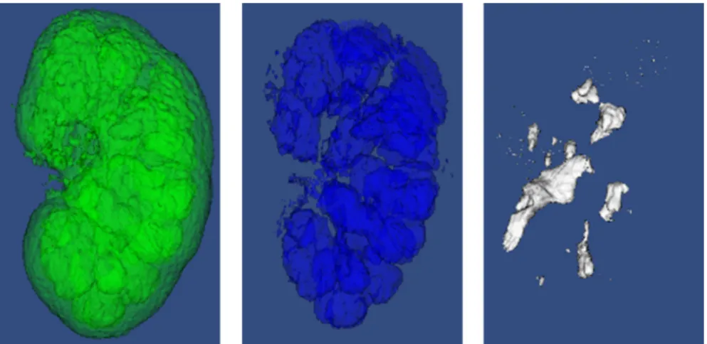
The results get from step 1) and 2) are illustrated in Fig.4. In this figure, we do not consider fat because it’s not useful for the illustration of the renal anatomical structure. We can see that the three materials are relatively independent from each other. At the border of two materials, the algorithm detects the surface for each of them respectively. That is to say, the algorithm cannot separate the surface inside and outside of the object and all of the borders are detected as surfaces. The three surfaces are rendered as three different objects with transparency properties and the final merged image is illustrated in Fig.5. From the results, we can see that the multi-object solution is practical for this situation. The advantage of this method is that the final image can be rendered very fast (> 24 Fps) after the surface extraction. The disadvantage is that the surfaces should be extracted first and the volumes are reduced to the boundaries of materials and all the other information is lost.
4.3. Volume rendering methods
We choose to perform direct volume rendering using ray casting. The framework of its rendering process is shown in Fig.6. As introduced before, the input of this rendering pipeline is the material probabilities on each voxel (Eq.1) and the material properties (color Ck and opacity value αk) assigned
by the user. The difficulty of the expansion from scalar volume to vectorial exists in the gradient computation and the transfer function design because the sample values are material probabilities and material properties instead of scalar values.
The sample positions depend on the direction of the casted rays. The material probabilities on the sample points are achieved by tri-linear inter-polation method. From the sampled material probabilities and the assigned material properties, we get the sample color Csand sample opacity αsfor the
composition step of the rendering pipeline. The sample color and opacity are given by a transfer function. Concerning the opacity, the transfer function can have two roles [6]: (a) assign to a specific voxel the tissue transparency and (b) enhance the surfaces by increasing the opacities in the boundary ar-eas and decrar-easing them in homogeneous regions. Different transfer functions will lead us to different direct volume rendering methods. Besides the trans-fer function, shading is another important issue in the rendering pipeline. Shading effects can be used to modulate the appearance of the samples. We apply the widely used Phong’s shading model [18] to calculate the shaded color. Both the calculation of transfer function and shading requires the gradient information.
4.3.1. Gradient estimation
Normally, for a scalar volume the gradient is approximated by intensity differences on each grid. But for the vectorial volume, the intensity differ-ences cannot be implemented as gradient information directly. Drebin et al. [19] proposed to form first a density volume by assigning a density value to each material and then composing the densities weighted by the materials’ probabilities. In his paper, a density characteristic ρk is assigned for the kth
material and then the density is formed by the following formula for each grid: D = K ∑ k=1 ρkpk (3)
We can see that the greater ρkis, the more important the kth material is.
If ρk equals to zero, the kth material will disappear in the final image. The
material opacity αk has the similar effect: αk = 1 implies that the material
is completely opaque, and αk = 0 implies that it is completely transparent
so that we can use the opacity αk to replace ρk to form the density volume.
This replacement can reduce the input parameters of the rendering pipeline so that it can simplify the user input because the two properties: opacity αk
D =
K
∑
k=1
αkpk (4)
Denote the gradient vector by G, and G = (Gx, Gy, Gz). Gx, Gy and Gz
are the directional gradient in x, y and z axis direction respectively. The gradient vector is calculated by 3D Sobel operator from the density volume
D. The normal direction is the gradient vector normalized by its magnitude |G|:
N = (Gx/|G| , Gy/|G| , Gz/|G|) (5)
4.3.2. Class decision method
When taking one sample during the ray casting process, the input are the material probabilities, it is natural to consider first to make a material decision from the pk’s (k = 1, . . . , K) and then to assign the corresponding
material properties to the sample point. This method is called class decision
method.
We first analyze the first derivate analysis of the material probabilities. Fig.7 shows the corresponding first order derivate of the result probabilities along one cut line (represented in white). We can see the border of two materials very clearly. At the boundary region, the positive derivate indicates that the line is going inside the material and the negative derivate indicates going out of the material. The first derivate tends to zero when the line passes inside of the materials. When we cast a ray into the volume, we calculate the first derivate along the ray. With the analysis before, we can easily distinguish the inside of the one material and the borders of materials. We can also get the information that we are going from material B to material A if the first derivate of A is positive and the first derivate of B is negative, as illustrated in Fig.7. Denote the directional first derivate of kth material as
f′(k), and the color and opacity of the kth material as Ckand αkrespectively,
the sample color Cs and the sample opacity αs are given by:
Cs= Cp αs= αp where p = arg max k
f′(k) (6)
With this formula, the inside of the materials will be discarded because the first derivate tends to zero. From Fig.7 we can see that the highest first derivate appears at the border of two materials which will give a high opacity
according to Eq.6. This formula defines a class decision for the boundary of two materials, so that it is called class decision method.
4.3.3. Composed color and opacity
Unlike the class decision method, the color and opacity for the sample position can be gotten from the material probabilities directly by multiplying the color and opacity assigned to that material by the probability of each material. The sample color Cs and the sample opacity αs are given by:
Cs= K ∑ k=1 Ckpk αs= K ∑ k=1 αkpk (7)
where pk denotes the probability of the kth material and the number of
materials is K.
As mentioned before, during the rendering process, the regions of interest are boundaries between materials and the transfer function is an efficient tool to express the boundaries [6]. Eq.7 has given out the color and opacity of the sample position, but it doesn’t have the ability to highlight any boundaries. The composed opacity has the same formula as the density volume (Eq.4). Fig.8 illustrates the relationship between the sample location and the first derivative of the density volume. The first derivate is actually just the gra-dient magnitude [20] (the gragra-dient computed on the densities D). We can see that the gradient magnitude magnifies at the material boundaries and equals to zero at the interior of one material, which is corresponding to the separated materials’ first derivative (Fig.7).
Usually the gradient magnitude is very sensitive to the noise, but due to the efficiency of neighborhood weighted classification method, the result of the classified material is almost homogeneous. As the density volume is con-structed according to the material opacities, the gradient magnitude agrees with the material opacity values. If two materials have similar opacities, the boundary between them will have small gradient magnitude; contrarily, if the two materials are quite different, the boundary between them will have a big gradient magnitude. The gradient magnitude can be considered as the ”importance” of a boundary surface. If we use the gradient magnitude as an opacity mask, all the boundaries will appear in the final image according to their ”importance”.
αs = ( K ∑ k=1 αkpk ) · |Gs|′ (8)
where|Gs|′ is the normalized gradient magnitude at the sample position,
it is given by:
|Gs|′ =
|Gs| − |G|min
|G|max− |G|min
(9)
where |G|max and |G|min denote respectively the global maximum and minimum gradient magnitude of the whole volume.
4.3.4. Volume rendering results
According to the framework described in Fig.6, we did some experiment on the classified kidney volume. The input is the material probabilities on each grid and the materials’ colors and opacities. The ”fat” material is useless for the observer, so a totally transparent property (opacity equals to zero) is assigned to it.
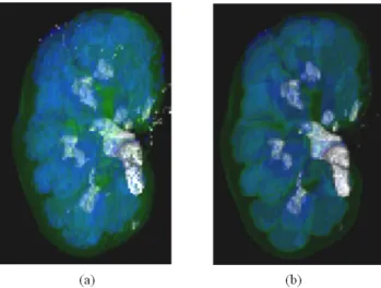
Fig.9 shows the difference between the two transfer function design meth-ods: Fig.9(a): class decision method and Fig.9(b): composed color and opac-ity. Comparing these two methods we can state the following remarks. In Fig.9(a) and (b), the same material properties are applied. On Fig.9(a), we can see that the class decision method can better discriminate the differ-ent material; there is less color confusion in the rendering result. But the decision making process is a 0-1 procedure so the rendering results appear discrete. In contrast, on Fig.9(b), the final result appears more continual because the boundaries are composed of two materials. To go further, the comparison between the three results (Fig.5 and Fig.9(a) and (b)) is rather delicate because of the subjectivity of any visualization evaluation. As men-tioned previously, the methods based on a decision (surface rendering and class decision method) give sharp boundaries and so seem to provide a more accurate visualization. However, this felt accuracy is totally subjective and depends entirely on the accuracy of the segmentation and the decision rules. Moreover, some pioneer works done in the early 90’s [21, 22] showed that methods based on the composition of color and opacity like direct volume rendering or our ”composed color and opacity” can give visualization results with more useful information than the decision based one. This assertion is based on the fact that on direct volume rendering the data is visually
analyzed and interpreted by the human psychovisual system and then some information can be perceived even if it cannot been formally extracted or described by a processing.
The computational costs of the two methods are almost the same because the difference of them only exists in the transfer function. For the volume rendering methods, the computation burden appears in the data resample part during data traversal. Every time the view direction changes, we need to recast the rays and perform the whole volume rendering process. So that comparing to the surface rendering method, low rendering speed is still a problem for volume rendering techniques. The improvement of the volume rendering speed is out of our discussion range in this paper. So that we use an eclectic method to interactively choose the appropriate visual direction: reduce resolution during the interactive process and back to resolution when the view direction is settled. The GPU based techniques [23] can be applied to speed up volume rendering and achieve real-time rendering speed.
5. Conclusions
With the development of 3D/3D medical image registration methods, more and more applications meet the requirement of the visualization of spatially-aligned volumes. Most of the existing methods for multi-volume visualization are based on the intermixing of the volumes at one certain step in the rendering pipeline. In this paper, we propose an acquisition level intermixing method, in which the intermixing step appears at the beginning of the rendering process.
First, the individual volumes are combined into a vector volume. The analysis is performed on this vectorial volume instead of several separated scalar volumes.
Then we performed a statistical vectorial volume classification method based on the Gaussian mixture model. But in order to integrate more infor-mation into the classification process, we propose a neighborhood weighted method for the analysis of the vectorial volume. The basic ideas of this method are that the voxels’ intensity vectors distribution can be modeled by a mixture of Gaussians and that the classes distributions on each voxel are affected by its neighbors’ class probability distributions. This neighbor-hood information is integrated into the classification process by amending the voxel’ s class distributions at each iteration step.
Then several rendering techniques are applied on the classification result. Both of the surface rendering and direct volume rendering techniques can be adapted to this situation. Two kinds of transfer design methods for direct volume rendering (class decision method and composed color and opacity) are implemented and compared. Similar to the single volume visualization techniques, the volume rendering method takes longer time to compute the final image because it requires to resample the whole dataset each time when the view direction changes. The rendering results of the two methods are given and the comparison of them is discussed.
From this framework, we can see that the rendering results rely much on the classification result because the final rendering techniques are ap-plied on the classification result. Comparing the traditional multi-volume visualization methods, in this framework, the rendering techniques play less important role. We can see that both surface rendering and volume rendering techniques can work well if the classification results are good. So that the key step of this framework becomes the classification instead of rendering, which should be further worked on.
6. Multi-volume rendering framework References
[1] Maintz, J.B., Viergever, M.A.. A survey of medical image registration. Med Image Anal 1998;2(1):1–36.
[2] Zitova, B., Flusser, J.. Image registration methods: a survey. Image Vision Comput 2003;21(11):977–1000.
[3] Hill, D.L., Batchelor, P.G., Holden, M., Hawkes, D.J.. Medical image registration. Phys Med Biol 2001;46(3):R1–45.
[4] Jannin, P., Grova, C., Gibaud, B.. Fusion de donn´ees en imagerie m´edicale: revue m´ethodologique bas´ee sur le contexte clinique. ITBM-RBM 2001;22(4):196 – 215.
[5] Betrouni, N.. Le recalage en imagerie m´edicale : de la conception `a la validation. IRBM 2009;30(2):60 – 71.
[6] Levoy, M.. Display of surfaces from volume data. IEEE Comput Graph Appl 1988;8(3):29–37.
[7] Levoy, M.. Efficient ray tracing of volume data. ACM T Graph 1990;9(3):245–261.
[8] Kaufman, A., Mueller, K.. The visualization Handbook; chap. Overview of volume rendering. Academic Press; 2004,.
[9] Hadwiger, M., Kniss, J.M., Rezk-salama, C., Weiskopf, D., Engel, K.. Real-time Volume Graphics. Natick, MA, USA: A. K. Peters, Ltd.; 2006.
[10] Cai, W., Sakas, G.. Data intermixing and multi-volume rendering. Comput Graph Forum 1999;18(3):359–368.
[11] Wilson, B., Lum, E., Ma, K.L.. Interactive multi-volume visualization. In: Computational Science - ICCS 2002; vol. 2330 of Lecture Notes in
Computer Science. Springer Berlin; 2002, p. 102–110.
[12] Roettger, S., Bauer, M., Stamminger, M.. Spatialized transfer func-tions. In: Eurographics-IEEE VGTC Symposium on Visualization. Leeds; 2005, p. 271–278.
[13] Firle, E.A., Keil, M.. Multi-volume visualization using spatialized transfer functions. gradient- vs. multi-intensity-based approach. In: CARS’07. Berlin; 2007, p. S121–S123.
[14] Tang, H., Dillenseger, J.L., Bao, X.D., Luo, L.M.. A vectorial im-age soft segmentation method based on neighborhood weighted gaussian mixture model. Comput Med Imag and Grap 2009;33(8):644–650. [15] Elvins, T.T.. A survey of algorithms for volume visualization. In:
SIGGRAPH ’92; vol. 26. Chicago: Computer Graphics; 1992, p. 194– 201.
[16] Tang, H., Dillenseger, J.L., Luo, L.M.. Intra subject 3D/3D kidney registration using local mutual information maximization. In: 29th conf. of the IEEE Engineering in Medicine and Biology Society. Lyon; 2007, p. 6379–6382.
[17] Lorensen, W.E., Cline, H.E.. Marching cubes: A high resolution 3D surface construction algorithm. In: SIGGRAPH ’87; vol. 21. Computer Graphics; 1987, p. 163–169.
[18] Phong, B.T.. Illumination for computer generated pictures. Commun ACM 1975;18(6):311–317.
[19] Drebin, R.A., Carpenter, L., Hanrahan, P.. Volume rendering. In: SIGGRAPH ’88; vol. 22. New York: Computer Graphics; 1988, p. 65–74. [20] Kindlmann, G., Durkin, J.W.. Semi-automatic generation of transfer functions for direct volume rendering. In: IEEE Symposium on Volume Visualization. 1998, p. 79–86.
[21] Vannier, M.W., Pilgram, T., Hidebolt, C., Marsh, J.L., Gilula, L.. Diagnostic evaluation of three dimensional CT reconstruction methods. In: CAR’89. Berlin; 1989, p. 87–91.
[22] H¨ohne, K.H., Bomans, M., Pommert, A., Riemer, M., Tiede, U., Wiebecke, G.. 3D Imaging in Medicine; vol. F 60; chap. Rendering tomographic volume data: adequacy of methods for different modalities and organs. NATO ASI Series,; 1990, p. 197–215.
[23] Kruger, J., Westermann, R.. Acceleration techniques for GPU-based volume rendering. In: 14th IEEE Visualization 2003 (VIS’03). Wash-ington, DC; 2003, p. 38.
List of Figures
1 Rendering pipeline for different intermixing levels . . . 19 2 Multi-volume rendering pipeline . . . 20 3 Registered slices from uro CT scans: a) unenhanced-, b)
nephrographic-and c) excretory-phase. d) Classification result: fat (red), re-nal cortex (green), rere-nal medulla (blue) and collecting system (white) . . . 20 4 Surface extraction result of the material probability volumes,
from left to right: renal cortex, renal medulla and collecting system . . . 21 5 Merged scene rendered by semi-transparent surface rendering
technique . . . 21 6 Volume rendering framework . . . 22 7 Probability first order derivate along one cut line. The
cir-cled region means the line goes from material B (red part) to material A (green part) . . . 22 8 The first derivative of the density volume . . . 23 9 Rendering results with the same material properties. (a):
Figure 2: Multi-volume rendering pipeline
Figure 3: Registered slices from uro CT scans: a) unenhanced-, b) nephrographic- and c) excretory-phase. d) Classification result: fat (red), renal cortex (green), renal medulla (blue) and collecting system (white)
Figure 4: Surface extraction result of the material probability volumes, from left to right: renal cortex, renal medulla and collecting system
Figure 6: Volume rendering framework
Figure 7: Probability first order derivate along one cut line. The circled region means the line goes from material B (red part) to material A (green part)
Figure 8: The first derivative of the density volume
Figure 9: Rendering results with the same material properties. (a): Class decision; (b): Composed color and opacity