for Visual Reasoning Tasks
Doctoral Dissertation submitted to the
Faculty of Informatics of the Università della Svizzera Italiana in partial fulfillment of the requirements for the degree of
Doctor of Philosophy
presented by
Sjoerd van Steenkiste
under the supervision of
Jürgen Schmidhuber
Cesare Alippi Università della Svizzera Italiana, Switzerland
Natasha Sharygina Università della Svizzera Italiana, Switzerland
Bernhard Schölkopf Max Planck Institute for Intelligent Systems, Germany
Michael C. Mozer University of Colorado Boulder, USA
Leslie P. Kaelbling Massachusetts Institute of Technology, USA
Dissertation accepted on 23 November 2020
Research Advisor PhD Program Director
Jürgen Schmidhuber Silvia Santini
I certify that except where due acknowledgement has been given, the work presented in this thesis is that of the author alone; the work has not been submit-ted previously, in whole or in part, to qualify for any other academic award; and the content of the thesis is the result of work which has been carried out since the official commencement date of the approved research program.
Simon Jacob “Sjoerd” van Steenkiste Lugano, 23 November 2020
Deep neural networks learn representations of data to facilitate problem-solving in their respective domains. However, they struggle to acquire a structured representation based on more symbolic entities, which are commonly understood as core abstractions central to human capacity for generalization. This dissertation studies this issue for visual reasoning tasks. Inspired by how humans solve these tasks, we propose to learn structured neural representations that distinguish objects: abstract visual building blocks that can separately be composed and reasoned with. We investigate the limitations of current deep neural networks at effectively discovering, representing, and relating these more symbolic entities, and present several improvements.
To address the problem of discovering and representing objects, we propose two novel approaches. In one case, we formalize this problem as a pixel-level clustering problem and formulate a neural differentiable clustering algorithm that solves it. We demonstrate how, unlike standard representation learning techniques, it can be trained to learn about objects in an unsupervised manner and acquire corresponding representations that can be treated as symbols for rea-soning. In the other case, we adopt a purely generative approach and demonstrate how a neural network equipped with the right inductive bias can learn about objects in the process of synthesizing images, even in complex visual settings.
Concerning the problem of relating symbolic entities with neural networks, we investigate how object representations can help facilitate building structured models for common-sense physical reasoning that generalize more systematically. We extend our previous representation learning approach to facilitate model building in this way and demonstrate how it can learn about general relations between objects to reason about their (future) physical interactions.
Finally, we investigate the utility of a representational format that isolates inde-pendent sources of information for encoding the features of individual objects. We conduct a large-scale study of such ‘disentangled’ representations that includes var-ious methods and metrics on two new abstract visual reasoning tasks. Our results indicate that better disentanglement enables quicker learning using fewer samples.
I would like to thank Jürgen Schmidhuber for providing me with the opportunity to pursue a PhD under his supervision, and for giving me the freedom to research the topics in this dissertation. Through our discussions, I learned to think critically and to develop my own understanding of AI.
Next, I would like to thank Klaus Greff in particular, for being my main collaborator and a friend throughout all these years. Several of the ideas we published together would not have existed if it were not for his initial curiosity and tenaciousness regarding the binding problem in neural networks. Through countless hours of discussion and collaboration, we went far beyond what I could have independently achieved.
I would also like to thank my other colleagues at IDSIA for providing an inspirational research environment throughout the years. It were the interactions with Jan Koutník, Bas Steunebrink, Rupesh Srivastava, and Marijn Stollenga that led me to join IDSIA, and with Paulo Rauber and Imanol Schlag that kept me going. I would also like to thank Paulo Rauber for feedback on this dissertation and Louis Kirsch, Aleksandar Stani´c, Róbert Csordás, and Anand Gopalakrishnan for collaborations.
Throughout my PhD, I was fortunate to intern at Google Brain in Zürich with Karol Kurach and Sylvain Gelly, which I would like to thank for this opportunity and as collaborators. I am also grateful for collaborations with many others at Google, including Olivier Bachem, Francesco Locatello, Thomas Unterthiner, Raphaël Marinier, and Marcin Michalski. I would like to thank Michael Chang for collaborating during his visit at IDSIA in the summer of 2018.
Many thanks go out to Kari for helping me balance work with much needed distraction during all these years, and to Wiebke for her patience and support. I would also like to thank Stefano and Dina for their continued support and good faith.
Finally, I would like to thank my brother, Job, and my parents, Ben & Marion, for their unconditional support and enthusiasm, and for all the memories we have made over the years. Without you, none of this would have been possible.
Contents vii
1 Introduction 1
1.1 Problem Statement and Contributions . . . 3
1.2 Structure of the Dissertation . . . 6
2 Background 9 2.1 Notation . . . 9 2.2 Machine Learning . . . 10 2.2.1 Statistical Modeling . . . 11 2.2.2 Classification . . . 19 2.3 Neural Networks . . . 20 2.3.1 Architectures . . . 21 2.3.2 Learning . . . 25
3 Challenges & Related Work 31 3.1 The Binding Problem . . . 33
3.1.1 Importance of Symbols . . . 33
3.1.2 Symbolic Processing in Connectionist Methods . . . 34
3.1.3 The Binding Problem in Connectionist Methods . . . 36
3.2 Representation . . . 39 3.2.1 Representational Format . . . 40 3.2.2 Representational Dynamics . . . 41 3.2.3 Methods . . . 43 3.3 Segregation . . . 48 3.3.1 Objects . . . 49 3.3.2 Segregation Dynamics . . . 51 3.3.3 Methods . . . 53 3.4 Composition . . . 59 3.4.1 Structure . . . 60 vii
viii Contents
3.4.2 Reasoning . . . 64
3.4.3 Methods . . . 66
3.5 Disentangling Factors of Variation . . . 71
3.5.1 Informative Factors of Variation . . . 71
3.5.2 Learning Disentangled Representations . . . 72
4 Neural Expectation Maximization 75 4.1 Method . . . 76
4.1.1 Neural Spatial Mixture Model . . . 77
4.1.2 Expectation Maximization . . . 77
4.1.3 Trainable Clustering Procedure . . . 79
4.1.4 Training Objective . . . 80 4.2 Related work . . . 82 4.3 Experiments . . . 83 4.3.1 Static Shapes . . . 84 4.3.2 Flying Shapes . . . 85 4.3.3 Flying MNIST . . . 87 4.4 Discussion . . . 89
5 Relational Neural Expectation Maximization 91 5.1 Method . . . 92
5.1.1 RNN-EM as a Predictive World Model . . . 92
5.1.2 Interaction Function . . . 95 5.2 Related Work . . . 97 5.3 Experiments . . . 99 5.3.1 Bouncing Balls . . . 100 5.3.2 Hidden Factors . . . 103 5.3.3 Space Invaders . . . 103 5.4 Discussion . . . 104
6 Object Compositionality in GANs 107 6.1 Method . . . 108
6.1.1 Generative Adversarial Networks . . . 108
6.1.2 Incorporating Architectural Structure . . . 109
6.2 Related Work . . . 113
6.3 Experiments . . . 115
6.3.1 Qualitative Analysis . . . 118
6.3.2 Quantitative Analysis . . . 121
7 Evaluating Disentangled Representations 127
7.1 Methodology . . . 128
7.1.1 Disentanglement . . . 129
7.1.2 Abstract Visual Reasoning . . . 130
7.2 Results . . . 134
7.2.1 Learning Disentangled Representations . . . 134
7.2.2 Abstract Visual Reasoning . . . 135
7.3 Discussion . . . 141
8 Conclusion 143 8.1 Future Directions . . . 146
A Additional Experiment Details 149 A.1 Neural Expectation Maximization . . . 149
A.1.1 Static Shapes . . . 149
A.1.2 Flying Shapes . . . 150
A.1.3 Flying MNIST . . . 151
A.2 Relational Neural Expectation Maximization . . . 152
A.2.1 Bouncing Balls . . . 152
A.2.2 Space Invaders . . . 154
A.3 Object Compositionality in GANs . . . 155
A.3.1 Model specifications . . . 155
A.3.2 Hyperparameter Configurations . . . 156
A.3.3 Instance Segmentation . . . 157
A.3.4 Human Study . . . 158
A.4 Evaluating Disentangled Representations . . . 160
A.4.1 Architectures . . . 160
A.4.2 Abstract Visual Reasoning Data . . . 162
B Additional Results 165 B.1 Object Compositionality in GANs . . . 165
B.1.1 FID Study . . . 165
B.1.2 Human Study - Properties . . . 168
B.1.3 Examples of Generated Images . . . 171
B.2 Evaluating Disentangled Representations . . . 186
B.2.1 Learning Representations . . . 186
B.2.2 Abstract Visual Reasoning . . . 188
Introduction
The study of Artificial Intelligence (AI) is concerned with programming machines to behave intelligently [Russell et al., 1995; Hutter, 2004]. Broadly speaking, such behavior is characterized by the capacity to achieve meaningful goals in a variety of situations, and by the ability to improve based on prior experiences. The most prominent examples of intelligent behavior are found among animals and humans, which have acquired general ‘programs’ throughout the course of evolution that enable them to learn from experiences and act as general problem solvers. In its most general form, the study of AI is therefore also concerned with certain aspects of neuroscience and cognitive psychology, which focus on understanding human intelligence and cognition.
The possibility of (an) AI to rival or surpass human capacity for problem-solving offers tremendous potential for automation and innovation in numerous domains. Conversely, the typical more ‘narrow’ approach to AI that is concerned with a particular domain, or problem setting, and that may sooner yield promising application, can serve as an intermediate step towards achieving this more general overarching goal. Indeed, several decades of AI research have led to significant advances in natural language understanding, computer vision, planning, and automated reasoning.
In recent years, artificial Neural Networks (NNs) have re-emerged as a promis-ing technique for AI in several of these domains [Schmidhuber, 2015a]. Modern NNs consist of simple connected nodes (neurons) organized in layers that each compute a non-linear transformation of their input (i.e. the output of the previous layer) based on the weights on the incoming connections. Like other Machine
Learning (ML) approaches [Mitchell et al., 1997], they can be programmed to
produce the desired input-output mapping (in this case by adjusting their weights) through learning from data. This makes it possible to teach NNs to perform tasks
2
that are otherwise difficult to manually program efficiently, such as recognizing objects in images, but for which corresponding data (e.g. in the form of correct input-output pairs) is more easily obtained.
Part of the reason for the success of recent ‘deep’ neural networks — neu-ral networks consisting of many layers — is that their intermediate layers form alternative descriptions, or representations, of the input data [Ivakhnenko and Lapa, 1965; Bengio et al., 2013]. Indeed, the importance of using the right representation (or features) for machine learning is well-established in the litera-ture [Murphy, 2012]. For example, a representation that focuses only on relevant information content is less susceptible to noise and generally easier to learn from. Similarly, when considering more abstract ‘high-level’ features that are robust to certain changes in the input, it becomes easier to learn programs that generalize to other inputs. It is for this reason that a lot of previous work in ML has focused on engineering input features, whose primary purpose was to enrich the input data based on prior knowledge about relevant aspects for solving a given task (e.g. Lowe [1989]; Dalal and Triggs [2005] for vision).
Deep neural networks are capable of learning representations of the input data together with the desired output for the task under consideration. This sig-nificantly reduces the need for feature engineering and has led neural networks to become the default choice for learning directly from unprocessed data, such as raw visual images [Ciresan et al., 2011, 2012; Krizhevsky et al., 2012; Sharif Razavian et al., 2014]. It also makes NNs an attractive choice for representation learning specifically, where the main goal is to learn useful representations of the input data for the purpose of some other ‘down-stream’ application [Lee et al., 2009; Bengio et al., 2013]. In this case, learning can take place through more generic unsupervised learning objectives that do not require access to data that is labeled or include rewards [Schmidhuber, 1991b, 1992c; Vincent et al., 2008]. This is highly advantageous, since human labor is costly, especially when considering that deep neural networks trained on unprocessed data require access to large amounts of inputs to even learn a single task. Nonetheless, in either of these cases, several key challenges remain.
One major challenge is that it can not be guaranteed that the desired represen-tation simply emerges as a by-product of learning, even when large amounts of su-pervised data are provided. Spurious correlations due to data set bias may corrupt the learned representation, while in other cases not enough data can be provided so that all possible invariances are observed. These issues are known to have impor-tant consequences for generalization, while at the same time being difficult to ad-dress during learning (since only a finite amount of data is considered) without in-corporating additional assumptions [Jo and Bengio, 2017; Lake and Baroni, 2018].
Indeed, in neural networks the quality of the learned representations is primar-ily due to inductive bias [Mitchell, 1980], requiring careful consideration of the neural network architecture, objective function, and optimization procedure.
A related challenge is encountered specifically in the unsupervised case, where representations are learned based on some auxiliary task. In this case, to ensure that the learned representations turn out useful for other down-stream tasks, it is important to incorporate prior knowledge (often based on assumptions) about how such tasks are solved and the corresponding utility of a particular representational format [Kansky et al., 2017; Locatello et al., 2018]. This then also implies a trade-off, where more useful representations can often be obtained by making additional assumptions about a particular task, but which may come at the cost of their relevance to other tasks. Striking the right balance between utility and generality is another challenge that must be addressed in this framework.
1.1 Problem Statement and Contributions
The central focus of this dissertation is on unsupervised representation learning for
(relational) reasoning tasks from vision1. The capacity to perform reasoning is a
core aspect of human cognition and an essential ingredient to how humans solve many everyday tasks. Traditionally, this has made reasoning one of the focus areas of AI [Russell et al., 1995]. In the real world, reasoning often proceeds from vision, which offers a rich source of information that can readily be obtained and is not contingent on any form of pre-processing. On the contrary, it is difficult to reason directly in terms of low-level features, such as the color values of individual pixels. This has led researchers to consider alternative representations based on manual feature engineering or large-scale supervised learning for the purpose of solving a specific task. Unfortunately, this approach is highly laborious and therefore difficult to extend to the much broader class of visual reasoning tasks as encountered in the real world, which makes unsupervised representation learning an important problem in this domain.
To arrive at a good representation for solving visual reasoning tasks (e.g. for common-sense physical reasoning) in the unsupervised case, we will draw inspiration from how humans learn to solve such tasks. In particular, we note how human perception is structured around the discovery and representation of objects, which serve as abstract ‘building blocks’ for many aspects of cognition [Spelke and Kinzler, 2007]. For example, they allow humans to view a complex visual
1We define reasoning as the process of making inferences about the world based on one’s
4 1.1 Problem Statement and Contributions scene in terms of separate (independent) parts and describe relations between them, which can then be reasoned with. Two important properties of objects for the purpose of representing complex visual information are their modularity and their generality. The former ensures that they can be composed in different ways to efficiently describe a variety of encountered scenes, which enables humans to reuse knowledge about an object across many different contexts. The latter implies that the notion of an object can be used to describe a wide variety of visual appearances according to a shared format, which allows them to easily be compared, and reasoned with.
We hypothesize that a representation based on objects2 offers similar benefits
to neural networks for visual reasoning tasks. Indeed, there are interesting paral-lels between the idea of incorporating ‘object representations’ (that are modular and can be composed) and the use of symbols in more classic symbolic approaches to AI [Nillson, 1980]. While the latter relied on hand-crafted symbols and rules of manipulation that required a prohibitive amount of human engineering, their underlying compositionality (due to treating reasoning as a symbol manipulation process) did allow them to generalize in predictable and systematic ways akin to humans. In contrast, while standard neural network approaches that learn repre-sentations are naturally able to overcome this issue of ‘symbol grounding’ (i.e. how to obtain abstractions that have meaning in the real world [Harnad, 1990]), their failure at generalizing more systematically suggest that they lack an inductive bias to acquire the ability to process information more symbolically [Lake and Baroni, 2018; Santoro et al., 2018b].
To this extent, we make the following contributions:
The Binding Problem in Artificial Neural Networks We investigate the inability
of existing neural networks to effectively form, represent, and relate symbol-like entities (i.e. objects). We propose that the underlying cause for this is the binding problem: The inability to dynamically and flexibly bind information that is distributed throughout the network. The binding problem affects their capacity to form meaningful entities from unstructured sensory inputs (segregation), to maintain this separation of information at a representational level (representation), and to use these entities to perform new inferences, predictions, and behaviors (composition). Based on connections to neuroscience and cognitive psychology (e.g. Treisman [1999]), where the binding problem has been extensively studied in
2We define objects as abstract patterns in the (visual) input that serve as modular building
blocks (i.e. they are self-contained and reusable independent of context) for solving a particular task, in the sense that they can be separately intervened upon or reasoned with.
the context of the human brain, we work towards a solution to the binding problem in neural networks and identify several important challenges and requirements. We also survey relevant mechanisms from the machine learning literature that either directly or indirectly already address some of these challenges. Our analysis provides a starting point for identifying the right inductive bias to enable neural networks to process information more symbolically and thereby generalize in a more systematic fashion.
Discovering and Representing Objects We propose two novel approaches to
discover and represent objects in a way that allows them to be treated as symbols for reasoning, unlike the representations learned by standard neural network approaches. Learning about objects is particularly difficult in the unsupervised case, where the notion of an object must be acquired solely through observing statistical regularities in the data. Moreover, due to the binding problem, it is not trivial how to best encode their information with a neural network.
In order to learn about objects, we will focus on their functional role as abstract computational units that are modular and reusable across many different contexts. In one case, this allows us to treat this problem as a pixel-level clustering problem, where pixels are related through belonging to the same cluster, and where each cluster corresponds to a particular object. We propose a trainable clustering procedure called Neural Expectation Maximization (N-EM) that can be formalized as maximum likelihood estimation (using generalized EM [Dempster et al., 1977]) in a spatial mixture model, where each component is parametrized by a shared neural network. The weights of the neural network act as the similarity function according to which to cluster pixels, and we demonstrate how one can backpropagate gradients through the generalized EM procedure so that they can be adjusted to learn about objects in a purely unsupervised fashion.
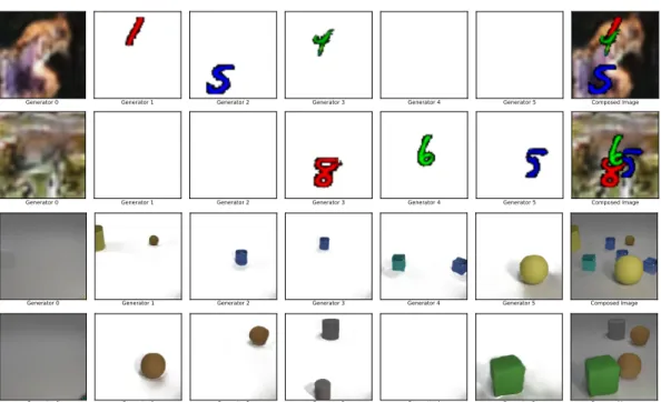
We also investigate an alternative approach to learning about objects based on more powerful implicit generative models. In this case, this requires learning a generative process that explicitly considers such abstractions at a representational level, which can be addressed by incorporating a corresponding inductive bias that encourages the learned generative process to be compositional. We propose a structured neural network generator that allows for compositionality in this way and demonstrate how it learns about objects, relations, and background. Using this approach, we find that it is possible to learn about objects in more complex visual settings that previous approaches (including N-EM) find difficult. We also demonstrate how to leverage the learned structured generative process, which is now interpretable and semantically understood, to perform inference and recover
6 1.2 Structure of the Dissertation information about individual objects without additional supervision.
Common-sense Physical Reasoning We propose a novel approach to learning
structured models for common-sense physical reasoning that takes advantage of the underlying compositionality of learned object representations to generalize in more predictable and systematic ways. To address this problem, a neural network should learn about possible relations between objects in a way that is general and reusable, and incorporate a mechanism for dynamically evaluating corresponding interactions at a representational level. Our neural approach combines N-EM with a compositional interaction function that is capable of modeling interactions between objects in this way. It decomposes complex interactions in the environ-ment into much simpler local pair-wise interactions between individual objects and dynamically decides which objects will interact. We demonstrate how this enables it to learn a structured world model capable of making predictions about physical interactions between objects, without access to supervision, in a way that applies to scenes consisting of more or fewer objects.
Abstract Visual Reasoning using Disentangled Representations We study the
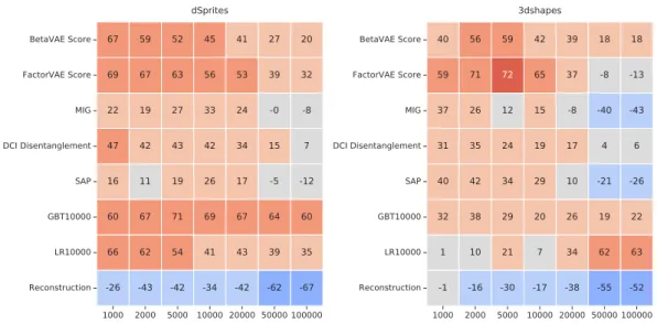
usefulness of representations that are disentangled, which provide a particular representational format for representing information about visual scenes. In a dis-entangled representation, information about informative factors of variation (e.g. the color, or shape of an object) can be readily accessed and is robust to changes in the input that do not affect this factor. While ‘disentanglement’ may be used to refer to different ways of imposing structure at a representational level, here we are mainly concerned with disentanglement as a way of encoding information about the features of individual objects. We conduct a large-scale evaluation of disentangled representations on two abstract visual reasoning tasks (similar to Raven’s Progressive Matrices [Raven, 1941]) that challenge the current capabil-ities of state-of-the-art deep neural networks. On these tasks, we demonstrate how representations that are more disentangled yield better sample-efficiency for learning the considered down-stream reasoning tasks.
1.2 Structure of the Dissertation
In Chapter 2 we provide a succinct overview of relevant concepts from statistical modeling and deep learning, which serve as technical background material. A reader that is already familiar with these concepts is welcome to skip this chapter or refer back to it on a case-by-case basis as indicated in the proceeding chapters.
In Chapter 3 we provide a detailed overview of the challenges and related work relevant to the topic of this dissertation. The focus of this chapter is on the binding problem, which will be introduced there since it provides a useful framework for identifying important challenges and requirements for incorporating object representations in neural networks. We also survey relevant mechanisms from the machine learning literature that either directly or indirectly already address some of these challenges. Towards the end of this chapter, we provide an overview of the challenges and related work for learning disentangled representations.
In Chapter 4 we introduce Neural Expectation Maximization (N-EM), which offers a trainable clustering approach based on neural networks. We demonstrate how N-EM is able to learn about objects in a purely unsupervised fashion and can be applied to images and videos to compute object representations.
In Chapter 5 we introduce Relational Neural Expectation Maximization (R-NEM), which combines N-EM with a relational mechanism to learn a structured model for common-sense physical reasoning. We demonstrate how it is able to leverage object representations to learn about physical interactions in a way that can be extrapolated to scenes consisting of more or fewer objects.
In Chapter 6 we introduce an alternative approach to learning about objects based on more powerful implicit generative models. In particular, we propose several modifications to a standard neural network generator to enable it to learn about objects, relations, and background, in the process of synthesizing complex visual scenes. We also demonstrate how to perform inference in this model and extract information about individual objects in unseen images.
In Chapter 7 we investigate the benefits of disentangled representations as a format for encoding information about individual objects on several abstract vi-sual reasoning tasks. We conduct a large-scale study that spans multiple different approaches to learning disentangled representations, notions of disentanglement, data sets and hyperparameters. We present compelling evidence that more disen-tangled representations are beneficial for down-stream abstract visual reasoning tasks in the few-sample regime.
Chapter 8 provides a summary of our contributions and offers an outlook on promising directions for future research.
Background
This chapter reviews background material on Machine Learning (ML) and Neural Networks (NNs) that is relevant to the methods developed in this dissertation. Regarding ML, most emphasis will be placed on unsupervised learning using sta-tistical models, while for NNs we limit ourselves to a discussion of basic concepts. The reader is referred to Bishop [2006]; Bousquet et al. [2011]; Goodfellow et al. [2016] for a more detailed exposition of these topics. Prior knowledge about probability theory and statistics is assumed and we recommend Casella and Berger [2002] for an overview.
2.1 Notation
Throughout this dissertation, we will adopt the following notation. We will write a variable x as x if it is a scalar, x for (column) vectors, and X for a matrix or higher-order tensor. Capital letters are used to denote scalar random variables, e.g. X , while vector-valued or higher-order random variables are written as X. Regarding the latter, we will clarify if X is a random variable or not if this is can not be determined from the surrounding context. Individual elements of vector-valued, or higher-order tensors (or random variables) are accessed via indices
i, j, k. For example, we will write Xi, j to refer to the i, j-th element of a matrix X. To select the j-th slice, we will write X:, j. In other cases, we will make use of
subscripts to denote separate variables e.g. x1, . . . , xN, which will be made clear from the surrounding context. The use of the element-wise product (or Hadamard product) will be indicated using , otherwise, the standard dot-product or matrix product is assumed.
We will write X ⇠ pXto denote that X is distributed according to the probability density (or mass) function pX. The dependency on X is typically clear from the
10 2.2 Machine Learning surrounding context and will normally be omitted. Similarly, depending on whether X is a discrete or a continuous random variable, we will use pX to either refer to a probability mass function (pmf) or probability density function (pdf). We will use the common shorthand p(x) to refer to p(X = x), which is the value of the pdf or pmf of a particular realization of X under pX. In certain cases, we will also write p(x) to refer to the function p(·) when this improves readability. The possible values that a random variable X can take will be denoted with calligraphy letters, e.g. X .
Often we will assume the existence of a ‘true’ or otherwise optimal value for a parameter ✓ , which will be denoted with an asterisk ✓⇤. The shorthand f
✓ is sometimes used to refer to a function f having parameters ✓ .
In all other circumstances, we will either make use of standard notation or clarify particular notation in the respective chapters.
2.2 Machine Learning
Machine learning is the field of research dedicated to the study of algorithms and statistical models that learn from data. At a high level, the ‘machine’ may be given by an agent, a model, or a function, whose behavior (output) in response to some input is governed by parameters. Learning then corresponds to the process of changing these parameters in relation to the observed data to achieve the desired behavior.
Broadly speaking, ML can be partitioned into supervised learning, unsuper-vised learning, and reinforcement learning1. The main distinction between
su-pervised and unsusu-pervised learning is due to requiring a data set containing correct input-output pairs in the supervised case. This makes it possible to apply supervised ML directly to learn to solve some task of interest, i.e. via classification (categorical output) or regression (real-valued output). In the unsupervised case, this is not possible, which typically limits its application to discovering patterns in the data to form alternative (potentially more effective) representations. On the other hand, since acquiring supervised data is costly, this alternative way of de-scribing the input data can have a profound impact on ‘down-stream’ applications that focus on prediction or analysis.
1For an overview of reinforcement learning, which is concerned with the study of agents that
interact with an environment according to a policy as to maximize a form of reward, we refer the reader to Kaelbling et al. [1996]; Sutton et al. [1998].
2.2.1 Statistical Modeling
In the context of unsupervised learning, we will primarily concern ourselves with statistical models in this work. Let D = {x1, x2, . . . , xN} be a sample drawn from a sequence of random variables X1, X2, . . . , XN that are independent and
identically distributed (i.i.d.) according to p(· | ✓⇤)2. Our goal is to model D with
a parametrized model m that specifies some probability distribution p(· | ✓, m) over X based on parameters ✓ 2 ⇥3. The probability distribution p(x | ✓, m) is
referred to as the likelihood, since it determines the likelihood of observing x under ✓ . The prior p(✓ | m) encodes our initial beliefs about likely parameter values before observing the data, which treats ✓ as a random variable.
Bayesian inference suggests a natural approach to unsupervised learning by computing the posterior distribution using Bayes’s rule, which updates our beliefs about the parameters upon observing the data:
p(✓ | D, m) = p(D | ✓, m)p(✓ | m)
p(D | m) . (2.1)
The posterior distribution p(✓ | D, m) tells us not only about the most likely parameter value that was used to generate D, but also provides a measure of uncertainty. The quantity in the denominator of (2.1) is referred to as the model
evidence (or as a marginal likelihood), which here acts as a normalization term
that is independent of ✓ . It can be computed by marginalizing (integrating) the joint likelihood p(D | ✓, m)p(✓ | m) over all possible parameter values ⇥. In order to make predictions about the probability of observing new data (that is i.i.d. as before) we can compute the posterior predictive:
p(x | D, m) =
Z ⇥
p(x | ✓, m)p(✓ | D, m)d✓. (2.2)
The posterior predictive weighs the likelihood of observing x under the current model using a particular choice of ✓ , by our beliefs about ✓ after observing D as encoded by the posterior (i.e. following the result of learning).
While making predictions using (2.2) (also known as the fully Bayesian ap-proach) is advantageous for a number of reasons [Bishop, 2006], it is usually difficult to compute the exact posterior due to the normalization term in (2.1). Therefore, a standard technique that we will adopt is to use a point estimate ˆ✓ in
2For simplicity we will mostly focus on the univariate case in this section, although it is
straightforward to extend these results to the multivariate setting.
12 2.2 Machine Learning place of the full posterior, such as the Maximum Likelihood (ML) estimate that is obtained by maximizing the likelihood function L(✓ | D, m) := p(D | ✓, m):
ˆ ✓M L := arg max ✓ L(✓ | D, m) = arg max✓ N Y i=1 p(xi| ✓, m). (2.3)
The maximum likelihood estimate corresponds to the largest mode of the posterior when assuming a Uniform prior for ✓ over ⇥. This makes it a natural choice, although note that normally ✓ is not treated as a random quantity in this framework. During learning it is often easier to use the (natural) logarithm of the likelihood to compute ˆ✓M L. The product of likelihoods in (2.3) then becomes
a sum, while monotonicity of the logarithm leaves the location of the maximum unchanged. When using a point estimate, the predictive distribution reduces to the likelihood of the model at the estimated parameter value.
Let us now briefly consider the following example of computing ˆ✓M L for a
Gaussian model, which will allow us to introduce some useful results for later in this dissertation.
Gaussian Example We assume that D = {x1, x2, . . . , xN} is an i.i.d. sample of
p(· | ✓⇤) and use a univariate Gaussian model with mean parameter µ, and variance 2, having the following probability density function:
N (x | µ, 2 ) := p12⇡exp ß 1 2 ⇣ x µ⌘2™ . (2.4)
For simplicity we will treat 2 as a fixed hyperparameter using 2
= 1, which leaves ✓ = µ. In this case, the likelihood becomes:
L(✓ | D) = N Y i=1 p(xi | ✓) = N Y i=1 1 p2⇡exp ß 1 2 (xi ✓ ) 2™ = 1 (2⇡)N/2exp ® 1 2 N X i=1 (xi ✓ )2 ´ , (2.5)
where we have left the dependence on the model m implicit.
In order to compute the ML estimate we will make use of (2.3), but then using the log of the likelihood:
ˆ ✓M L= arg max ✓ log L(✓ | D) = arg max ✓ N 2 log 2⇡ 1 2 N X i=1 (xi ✓ )2 = arg min ✓ 1 2 N X i=1 (xi ✓ )2 = arg min ✓ 1 2 N X i=1 (xi x)¯ 2+12 N X i=1 (¯x ✓ )2 Ç with ¯x = N1 N X i=1 xi å = N1 N X i=1 xi. (2.6)
In some cases, as we will encounter, it will be more difficult to compute these estimates analytically. Using gradient-based optimization may then provide a good alternative. The gradient of the log-likelihood of a univariate Gaussian model with fixed variance and mean parameter ✓ = µ is given by:
d d✓ log L(✓ | D) = d d✓ ñ N log p2⇡ 1 2 N X i=1 Å xi ✓ã2ô = 12 N X i=1 d d✓ Å xi ✓ã2 = N X i=1 Å xi ✓ 2 ã . (2.7)
Notice how this gradient points in the direction of ˆ✓M L, which in this case is
given by the sample mean.
Latent Variable Models
The purpose of statistical modeling usually varies between tasks. In some cases the primary goal of learning is density estimation, i.e. accurately estimating the prob-ability density function (or pmf in the case of discrete observations) from which the observed data was generated. In other cases, the emphasis is on uncovering ‘hidden’ latent structure in the data or representation learning. Representations are alternative ways of describing the data that focus on particular properties,
14 2.2 Machine Learning which will be of primary interest in this dissertation. The prototypical unsuper-vised learning techniques to learning representations focus on dimensionality reduction and clustering, which can be expressed using latent variable models that additionally include unobserved latent variables.
Consider a latent variable model of the form p(x, z | ✓) = p(x | z, ✓)p(z), where X captures the observed data, Z the unobserved latent variables, and ✓ 2 ⇥ are the parameters as before. In order to use this latent variable model to model
p(· | ✓⇤) we need to integrate over all possible values that Z can take:
p(x | ✓) = Z Z p(x, z | ✓)dz = Z Z p(x | z, ✓)p(z)dz. (2.8)
The assumptions about the interaction between Z and X dictate the structure of the model, and thereby of the learned representation. For example, if we assume that Z is a K-dimensional binary random variable that can take on K possible one-hot encoded states, and that the conditional likelihood p(x | Zk= 1, ✓k) is Gaussian, then we recover the well-known Gaussian Mixture Model (GMM):
p(x | ✓ ) =
K X
k=1
N (x | Zk= 1, µk, 2k)p(Zk= 1 | ⇡k). (2.9) In this model, we have K sets of parameters ✓ = {(µ, 2)
1, . . . , (µ, 2)K} for the
conditional likelihood and the latent variable Z determines which were used to generate x. The prior p(z | ⇡), having parameters ⇡, encodes our initial beliefs about the proportion of data assigned to each component. In order to perform inference about z we can compute the posterior p(z | x, ✓ , ⇡), which tells us which of the Gaussian components (clusters) x is expected to belong to. Together with the learned cluster centers µ1. . . µK and variances 2
1. . . 2K this provides an alternative description for x. Indeed, we will explore an adaptation of standard GMMs for representation learning in Chapter 4.
Another relevant model that we will make use of in this dissertation is based on the linear Gaussian model. In this case, we assume that Z is Gaussian and that the conditional likelihood p(x | z, ✓ ) is also Gaussian, but that its mean linearly depends on z through the matrix W of parameters:
p(x | ✓ ) =
Z Z
N (x | W z, ⌃)N (z | µz, ⌃z)d z. (2.10)
where ✓ = (W, ⌃) and ⇡ = (µz, ⌃z). If x is high-dimensional and z of lower
dimension, then we can think of z as being a compressed representation of x that can be inferred (after learning ✓ ) by computing p(z | x, ✓ , ⇡). Several other
models used for representation learning, such as Factor Analysis and Probabilistic PCA, have a similar functional form [Roweis and Ghahramani, 1999].
Expectation Maximization In principle, we can make use of the same techniques
from Bayesian inference to perform unsupervised learning and make predictions when using latent variable models. However, unlike before, log p(x | ✓) now includes an integration (or summation) term, which complicates maximization with respect to ✓ .
An alternative approach to Maximum Likelihood Estimation (MLE) for latent variable models (that is typically easier to work with) can be obtained by formu-lating a lower-bound based on some auxiliary distribution q:4
log p(x | ✓) = log Z Z p(x, z | ✓)dz = log Z Z q(z)p(x, z | ✓) q(z) dz Z Z q(z) logp(x, z | ✓)q(z) dz. (2.11)
where the final expression is obtained by applying Jensen’s inequality. This enables us to increase the data log-likelihood log p(x | ✓) and fit the model by maximizing (2.11) with respect to ✓ .
In order to determine how to choose q, we can make the following observation:
q⇤= arg max q(z) Z Z q(z) logp(x, z | ✓) q(z) dz = arg max q(z) Z Z q(z) log p(x | ✓) + q(z) logp(z | x, ✓)q(z) dz = arg max q(z) Z Z q(z) logp(z | x, ✓) q(z) dz = arg min q(z) DK L[q(z) || p(z | x, ✓ )] = p(z | x, ✓ ). (2.12)
where DK L[q || p] =RZq(z) log q(z)/p(z | x, ✓)dz is the KL divergence, which is minimized if and only if both distributions are identical. Hence, (2.11) is
4The conceptually simpler alternative of using Monte Carlo to approximate the
expecta-tion Ep(z)[p(x | z, ✓ )] with a sample average is extremely sample inefficient when x is high-dimensional [Doersch, 2016].
16 2.2 Machine Learning maximized wrt. q when choosing q(z) = p(z | x, ✓). In fact, it is easy to see that in this case the lower-bound is tight:
log p(x | ✓) Z Z q(z) logp(x, z | ✓)q(z) dz = Z Z p(z | x, ✓) log p(x | ✓)dz = log p(x | ✓). (2.13)
Together, these results suggest a simple iterative algorithm to maximizing log p(D | ✓) wrt. ✓, which is known as the Expectation Maximization algorithm [Dempster et al., 1977]. In each iteration, we first compute the E-step for each observation xi 2 D based on the previous parameter estimate ✓old (here we assume a single i.i.d. latent variable Zi for each observation), which tightens the lower-bound in (2.11) while holding the parameters fixed:
qi= arg max qi(zi) ñZ Zi qi(zi) logp(xi , zi| ✓old) qi(zi) dzi ô = p(zi | xi, ✓old). (2.14) Next, we compute the M-step, which produces a new parameter estimate by maximizing (2.11) wrt. ✓ across the data set:
✓ = arg max ✓ ñX i Z Zi qi(zi) logp(xi, zi| ✓) q(zi) dzi ô = arg max ✓ ñX i Z Zi
p(zi| xi, ✓old) log p(xi, zi | ✓)dzi ô
.
(2.15)
By iterating this EM algorithm until convergence, we are guaranteed to find a local optimum of the data log-likelihood [Wu, 1983]. However, it can sometimes still be difficult to analytically compute (2.15). In this case, we can use a gradient-based approach (similar to before), where we update ✓ in the direction of steepest ascent by differentiating (2.15) (optionally using a Monte Carlo approximation of the expectation). This procedure, which we will make use of in Chapter 4, is sometimes referred to as generalized EM.
Variational Inference
When using latent variable models for representation learning, we will some-times make us of Variational Inference (VI) [Wainwright and Jordan, 2008] (see
Blei et al. [2017]; Zhang et al. [2018a] for more recent overviews). It provides a framework for approximating the posterior distribution over a set of unobserved latent variables p(z | x, ✓) by an approximate ‘variational’ distribution q. In this case, inference can be treated as an optimization problem where the goal is to find a good approximate distribution q from a family of distributions Q over Z that minimizes some divergence between itself and the true posterior. The standard choice of divergence is the reverse KL-divergence, which yields the following optimization problem:
q⇤= arg min
q2Q DK L[q(z) || p(z | x, ✓ )]. (2.16)
The accuracy of the approximation is determined both by the flexibility of the distributions in Q, and by the ability to perform the optimization adequately. Although it is possible to use other divergences to perform variational inference (including the forward KL [Minka, 2001]), we will make use of the reverse KL, which has a closer resemblance to EM, as we will see next.
Note that it is not possible to optimize (2.16) directly due to its dependence on the marginal likelihood p(x | ✓) (here due to marginalizing Z), which is usually intractable to compute and the main reason that we can not use the exact posterior in the first place. Indeed, we have that:
DK L[q(z) || p(z | x, ✓ )] =
Z Z
q(z) log q(z) q(z) log p(x, z | ✓)dz + log p(x | ✓)
= LE LBO(q, ✓ ) + log p(x | ✓ ),
(2.17) where LE LBO is known as the Evidence Lower Bound (ELBO), defined as:
LE LBO(q, ✓ ) := Z Z q(z) log p(x, z | ✓) q(z) log q(z)dz = Z Z q(z) log p(x | z, ✓)dz DK L[q(z) || p(z)]. (2.18)
Because log p(x | ✓) acts as a constant in this optimization problem, we can now optimize (2.16) by maximizing the ELBO wrt. q. Moreover, by moving LE LBO(q, ✓ ) to the left-hand side in (2.17), it can also be seen how the ELBO forms a valid lower-bound to log p(x | ✓) (hence the name) as the KL-divergence is always positive.
18 2.2 Machine Learning Indeed, we note how the ELBO closely relates to our previous result for EM in (2.11), which was obtained by attempting to estimate the parameters of a latent variable model, i.e. to increase the marginal log-likelihood log p(x | ✓) wrt. ✓. Meanwhile, the ELBO was obtained by attempting to find an accurate variational approximation to the posterior p(z | x, ✓), i.e. to minimize DK L[q(z) || p(z | x, ✓ )] wrt. q. It turns out that these different optimization problems can be related through (2.17) and give rise to a similar objective.
It is straightforward to make use of this connection. In the E-step (2.14) of EM we found that we could tighten the lower-bound on log p(x | ✓) by choosing
q⇤= p(z | x, ✓ ). Hence, if this is not possible, for example, because it is intractable to compute the exact posterior under the current model, then it can now be seen how we can use a variational approximation to the posterior by using the ELBO to optimize q. This gives rise to the Variational Expectation Maximization algorithm, which uses (2.18) to minimize the variational objective in (2.16) in the E-step5.
Choosing a flexible family of variational distributions Q that also yields tractable optimization of the ELBO may still require careful inspection of the model. An alternative approach is to use “black-box” variational inference using a parametrized family of distributions Q = {q(· | ) : 2 ⇤} [Ranganath et al., 2014]. In this case, we can optimize by treating the integral in (2.18) as an expectation and use Monte Carlo approximation to compute stochastic gradients. Unbiased low variance gradients can often be obtained for continuous latent variables by using the ‘reparametrization trick’ [Kingma and Welling, 2014].
In the standard VI framework, the optimization problem in (2.16) is solved for each sample individually and therefore qi need not functionally depend on the actual observation. On the other hand, this makes plain VI computationally expensive for learning on large data sets. An alternative approach is to use an
inference model f : x 7! (e.g. a neural network having weights ) that amortizes
variational inference over an entire data set [Gershman and Goodman, 2014]. The inference model outputs variational parameters i for a given observation xi to implement q(· | xi, i). The parameters of the model are trained to optimize (2.16) for all data points simultaneously.
Variational Auto Encoder A well-known framework, which we will make use
of in Chapter 7 for representation learning, is that of Variational Auto-Encoders (VAEs) [Kingma and Welling, 2014]. VAEs employ amortized variational inference
5Note that the use of VI is not limited to finding ML estimates in latent variable models as
is EM. Rather, VI can be used to perform learning in fully Bayesian models, where the model parameters are themselves treated as latent variables that are optimized via (2.16).
using inference models to learn a statistical latent variable model of the observed data. The model is similar to the Linear Gaussian model in that it assumes a con-tinuous vector-valued random variable Zi for each observation and a conditional likelihood (often Gaussian) whose parameters depend on zi. However, unlike in the linear case, it uses a neural network f✓ to implement this mapping. This makes exact posterior inference intractable and amortized variational inference is used to approximate the posterior. The inference model in this case is also implemented by a neural network f , which allows (2.18) to be interpreted as a regularized auto-encoding objective: an observation is ‘encoded’ by the inference model to obtain q(zi | f (xi)) (from which we can sample zi) and then ‘decoded’ by the model to obtain p(xi | f✓(zi)) to evaluate the first term. The KL-term then acts as the regularizer. Typically the dependence on the neural network is left implicit and we will write q (zi | xi) and p✓(xi| zi) in this case as shorthand.
2.2.2 Classification
In other parts of this dissertation we will make use of supervised learning for classification tasks [Bishop, 2006]. We will also adopt a statistical approach in this case, and assume that D = {(x1, y1), (x2, y2), . . . , (xN, yN)} is a sample drawn from a sequence of random variables (X1, Y1), (X2, Y2), . . . , (XN, YN) that are i.i.d. according to p(x, y | ✓⇤). Since we are concerned with classification, the Yi are discrete random variables that each take on one of {0, 1, . . . , C 1} values (class labels). Our goal will be to learn a function h : X 7! Y (the classifier) which assigns the correct label y to any (new) observation x that is drawn from the corresponding conditional distribution.
In order to decide about h we introduce a loss function L : Y ⇥ Y 7! R, which measures how different the prediction ˆyi is from the true class yi for an observation xi. Next, we let the risk associated with h be given by:
R(h) =
Z X
Z Y
L(ˆy, y)p(x, y)d yd x. (2.19)
This then gives rise to a natural optimization objective for learning h 2 H , i.e. find the h that minimizes the risk. In most problems p(x, y) is not available and we will resort to minimizing the empirical risk based on D (i.e. the training data) in stead: Remp(h) = 1 N N X i=1 L(ˆyi, yi). (2.20)
20 2.3 Neural Networks Notice how, in this case of Empirical Risk Minimization (ERM), we are prone to an issue known as overfitting. Depending on the function class H , it may be possible to minimize Remp(h) in a way that does not generalize to new instances drawn from the same distribution. Similarly, it may occur that the sample D that is available to us was obtained with low probability (i.e. it is not representative) and can mislead the classifier. The framework of Probably Approximately Correct
(PAC) learning is concerned with providing guarantees about generalization for a
particular hypothesis class in these situations, and we refer the reader to Shalev-Shwartz and Ben-David [2014] for an overview. In this work, we will protect against overfitting by measuring the capacity to generalize explicitly using a separate validation data set, which is standard practice.
There exist multiple approaches to minimizing Remp [Bishop, 2006]. One approach is to learn a discriminant function that directly maps inputs to outputs. Another common approach, which we will make use of in this work is to learn a discriminative model that models the posterior class probabilities p(y | x, ✓) directly (the class label with the highest probability is chosen as the output). In this case, we can choose L as the negative log-likelihood and empirical risk minimization becomes equivalent to maximum likelihood estimation of ✓ . As we will see, it is natural to train neural networks in this way, i.e. when treating their output for a given input x as a probability distribution over Y . Finally, one can attempt to model the joint p(x, y | ✓) in its entirety and use Bayes’ rule to derive the posterior class probabilities, which will additionally incorporate uncertainty about ✓ and help against overfitting. However, similar to before, the issue of obtaining the marginal likelihood prevents us from using this approach in practice.
2.3 Neural Networks
In this disseration, we will focus heavily on machine learning using artificial Neural Networks (NNs). Generally speaking, NNs consist of simple connected nodes (neurons) that each compute an activation. Inputs may be received directly from the environment (e.g. sensory inputs) or indirectly in the form of the outputs (activations) of other nodes in the network. A real-valued multiplicative weight is associated with each connection that, together with its input, determines the activation of each neuron. The activation of a subset of the neurons is treated as the output of the network, which can be adjusted by changing the neural network weights. Hence, it is useful to think of neural networks as simply implementing a mapping from input to output, based on the value of its weights.
In modern neural networks [Schmidhuber, 2015b], neurons are organized in layers, such that each node in a layer is only connected to nodes in the previous layer. Deep neural networks consist of many layers of non-linear transformations and their ‘depth’ is determined by the number of consecutive layers that are used6.
Hence, deep neural networks can be viewed as successively transforming the input data to produce the desired output. In this case, the activations of the nodes in each intermediate (or ‘hidden’) layer provide an alternative representation of the input data, where each successive transformation contributes towards a representation that is better suited to produce the desired output [Lee et al., 2009]. This has recently allowed deep neural networks to overcome the limitations of manual feature engineering in several application domains (e.g. Fernández et al. [2007]; Ciresan et al. [2011]; Hinton et al. [2012]; Ciresan et al. [2012]; Krizhevsky et al. [2012]; He et al. [2017]). More important in the context of this work, is that (deep) neural networks learn representations that are also useful for solving other (related) tasks (e.g. Rumelhart et al. [1985]; Schmidhuber [1991a]; Zemel and Hinton [1994]; Bengio et al. [2013]; Zeiler and Fergus [2014]). This allows us to apply them for representation learning purposes directly, which will be our main use case in this work.
2.3.1 Architectures
Many different types of neural network architectures exist. Early approaches were often designed to function as (somewhat) plausible computational models of the human brain and include a number of specific components [Rosenblatt, 1958; Fukushima, 1980]. In contrast, the more modern architectures that we will consider mostly differ in how they combine a number of standard layers that essentially function as composable building blocks. These have little resemblance to how the human brain processes information, although there is evidence that in some cases similar activation patterns can be obtained during information processing [Yamins et al., 2013; Nayebi et al., 2018].
At a fundamental level, one can distinguish between feedforward neural
net-works and recurrent neural netnet-works. In feedforward neural netnet-works the first
layer receives its input directly from the environment, and the activations of the neurons in the final layer serve as the output of the network. Recurrent Neural Networks (RNNs) additionally incorporate circular dependencies between nodes that are resolved through time. Depending on the choice of architecture and
6Recently, this has popularized the term deep learning to refer to machine learning using deep
22 2.3 Neural Networks availability of data, feedforward neural networks are in principle able to learn any required transformation of the input data [Hornik, 1991; Lu et al., 2017], while an RNN can in principle simulate any Turing machine [Siegelmann and Sontag, 1991].
In the following, we will briefly introduce several standard neural network architectures that we will make use of throughout this dissertation. Variations on these architectures can be obtained by mixing and combining different layer types. We refer the reader to Goodfellow et al. [2016] for a more detailed overview.
Multi-Layer Perceptrons
Fully-connected layers are the basic building block of many modern neural net-work architectures. In a fully-connected layer, every unit in a layer receives as input the output of every unit in the previous layer. A well-known architecture that consists of L ‘hidden’ layers and an output layer that are fully-connected is the Multi-Layer Perceptron (MLP). In an MLP the jth unit in layer l computes:
z(l) j = N 1 X i=0 W(l) i, j · a(l 1)i + b(l)j , (2.21) a(l) j = (z(l)j ), (2.22)
where W(l)2 RN⇥M contains the weights on the edges from units i in layer l 1
to units j in layer l, and b(l) 2 RM contains the bias for units j in layer l. Here a(l 1)2 RN is the output of the previous layer l 1, where a(0)= x acts as the
input layer, and ˆy = a(L+1) as the output. Together, the weights and biases of
each unit in each layer form the parameters of the MLP.
Activation Functions The quantities z(l)
j and a(l)j are sometimes referred to as the pre-activation and the activation of a unit. The latter is obtained by applying an
activation function to each unit. Standard activation functions we will make use of include the Sigmoid: 1/(1 ez
), the Hyperbolic Tangent: tanh(z), the Rectified
Linear Unit (ReLU): max(0, z) [von der Malsburg, 1973], and variations on the
ReLU, such as the Leaky ReLU [Maas et al., 2013] and the Exponential Linear Unit (ELU) [Clevert et al., 2015].
It is important to note that when using a linear activation function, i.e. (z) =
z, the discriminative power of an MLP with multiple hidden layers is equivalent
to that of an MLP with a single hidden layer7. Hence, usually takes the form of
a non-linearity in order to make effective use of the depth of the network.
Output Layers The dimensionality of the output layer and its activation function
typically depends on the task itself, especially since we will often treat neural network outputs as implementing probability distributions. In a binary classifica-tion setting, where inputs x are said to either belong to class Y = 0 or Y = 1, the output layer consists of a fully-connected layer with a single unit and a Sigmoid activation function. The output of the network ˆy can then be interpreted as the
probability that the input belongs to the first class:
p(Y = 0 | x) = ˆy and p(Y = 1 | x) = 1 ˆy. (2.23)
Alternatively, this can be viewed as the network f✓ parametrizing a Bernoulli random variable Y ⇠ Bernoulli(p = f✓(x)). Notice also the similarity between an MLP that computes the output for a given input in this way, and the well-known
logistic regression model [Bishop, 2006].
In a multi-class classification setting where Y = {0, 1, . . . , C 1}, which we will explore in Chapter 7, we will let the network implement a categorical distribution in a similar fashion. In this case, the activation function needs to consider the pre-activation of all output neurons simultaneously in order to obtain a valid probability mass function. More specifically, for a classification problem having C classes, the output layer consists of a (fully-connected) layer with C units and the following softmax activation function [Bridle, 1990]:
p(Y = j | x) = softmax(zj) = e
zj
PC 1 j0=0ezj0
. (2.24)
In this case, the possible values Y can take are essentially one-hot encoded by the output neurons.
In other settings, like when using a neural network to implement a conditional Gaussian distribution N (x | f✓(z)), we will take a similar approach. We will let the output of the neural network correspond to the parameters of the corresponding distribution (in this case µ, 2), which will then dictate the choice of activation
function or output dimensionality.
Convolutional Neural Networks
When modeling images we will often make use of Convolutional Neural Networks (CNNs) [Fukushima, 1979; Waibel et al., 1989; LeCun et al., 1989, 1998]. The basic building block of a CNN is the convolutional layer whose activation A(l)2
differences in error back-propagation and the resulting credit assignment [Baldi and Hornik, 1995].
24 2.3 Neural Networks Rhl⇥wl⇥cl is given by a three-dimensional volume. Here h
l and wl are the spatial dimensions whose size is derived from the corresponding spatial dimensions of the input image, and cl is the feature dimension.
The computations of a convolutional layer are best described at the level of two-dimensional activation maps A(l)
c 2 Rhl⇥wl. Each map contains the activations of the neurons that are co-located in the feature dimension. Neurons that belong to this same feature map share their weights, hence the naming of this dimension as the feature dimension. The activation of a neuron at spatial location (i, j) in A(l)
k is computed as a weighted sum of the activations of the neurons in the previous layer at the same spatial locations (i, j) and the surrounding neighborhood. In other words, the activations in feature map k are obtained by first convolving a kernel W(l)
k 2 Rkh,kw,cl 1 with A(l 1) across the spatial dimensions, followed by a sum across the feature dimension (and adding a bias term for each feature). Here
kh, kw are the width and height of the kernel (hyperparameters) that determine the size of the neighborhood, and cl 1 is the number of feature maps in the previous layer.
It is desirable in a CNN to gradually decrease the size of the spatial dimensions with each consecutive layer as a means of increasing their receptive field and encourage more global (hierarchical) features to be learned [Fukushima, 1979; LeCun et al., 1989]. The approach that we will make use of in this case is to use
strided convolutions, where the kernel is applied only at regular intervals along
the spatial dimensions.
Note that it is trivial to combine convolutional layers with fully-connected layers via reshaping. In that sense, convolutional layers are also compatible with the fully-connected output layers discussed previously. Similarly, a convolutional layer may itself act as the output layer by appropriately choosing the output dimensionality and activation function as before.
Weight-sharing across the spatial dimensions as encountered in CNNs provides an inductive bias that is particularly helpful when processing images. In particular, this spatial invariance in lower layers makes it easy to learn features that capture local image statistics, such as edges or other local patterns, that can be re-used across a variety of image locations [Lee et al., 2009; Zeiler and Fergus, 2014]. Meanwhile, higher layers that act on the image more globally (i.e. due to having a larger receptive field) are able to learn more specialized (hierarchical) features, such as a ‘face feature’ [Lee et al., 2009], that use low-level features as building blocks.
Recurrent Neural Networks
The neural network architectures discussed previously only propagate information forward. A Recurrent Neural Network (RNN) also incorporates cyclic dependen-cies that are resolved through time [McCulloch and Pitts, 1943; Kleene, 1956; Werbos, 1988; Hochreiter and Schmidhuber, 1997; Gers et al., 2000; Chung et al., 2014]. From this perspective, an RNN can also be viewed as a dynamical system whose state evolves over time and which can function as a type of memory when processing sequential inputs [Schmidhuber, 1992b; Hochreiter and Schmidhuber, 1997].
Although an RNN can incorporate a number of fully-connected, convolutional, or other layers, it includes at least one recurrent layer. The most basic RNN consists of a single fully-connected recurrent layer that computes:
zj[t] = N 1 X i=0 Wi, j· xi[t] + M 1 X i=0 Ri, j· aj[t 1] + bj, (2.25) aj[t] = (zj), (2.26)
where W 2 RN⇥M contains the weights on the edges from units i in the input layer to the hidden units j, R 2 RM⇥M contains the weights on the edges from the hidden units i at time-step t 1 to hidden units j at time-step t, and b 2 RM contains the bias for the hidden units j. Here x [t] 2 RN is the input (layer), z[t] 2 RM the pre-activations, and a[t] 2 RM the activations at timestep t. The output of the RNN at timestep t are given by the activations a[t], although more commonly a fully-connected output layer is used to decouple the dimensionality of the hidden state (the memory) from the task under consideration.
The weights of the RNN are shared across time, which is an architectural inductive bias that simplifies learning solutions that are invariant across time. Moreover, this makes it possible to apply and train RNNs on sequences of varying time-length. A common choice of activation function is the Sigmoid, which squashes the pre-activation to [0, 1] and prevents the activations from ‘exploding’ when increasing the sequence length.
2.3.2 Learning
In order to train neural networks, we will make use of a loss function L(✓ , D) that relates the neural network weights and the observed data. The goal of learning is then to find the neural network weights ✓ that minimizes L(✓ , D). Due to the non-linearity of neural networks, it is usually not possible to solve for ✓