A Comparative Evaluation of the Performance of Passive and Active 3-D Vision Systems

READ THESE TERMS AND CONDITIONS CAREFULLY BEFORE USING THIS WEBSITE. https://nrc-publications.canada.ca/eng/copyright

Vous avez des questions? Nous pouvons vous aider. Pour communiquer directement avec un auteur, consultez la

première page de la revue dans laquelle son article a été publié afin de trouver ses coordonnées. Si vous n’arrivez pas à les repérer, communiquez avec nous à PublicationsArchive-ArchivesPublications@nrc-cnrc.gc.ca.

Questions? Contact the NRC Publications Archive team at

PublicationsArchive-ArchivesPublications@nrc-cnrc.gc.ca. If you wish to email the authors directly, please see the first page of the publication for their contact information.

NRC Publications Archive

Archives des publications du CNRC

This publication could be one of several versions: author’s original, accepted manuscript or the publisher’s version. / La version de cette publication peut être l’une des suivantes : la version prépublication de l’auteur, la version acceptée du manuscrit ou la version de l’éditeur.

Access and use of this website and the material on it are subject to the Terms and Conditions set forth at

A Comparative Evaluation of the Performance of Passive and Active 3-D

Vision Systems

El-Hakim, Sabry; Beraldin, Jean-Angelo; Blais, François

https://publications-cnrc.canada.ca/fra/droits

L’accès à ce site Web et l’utilisation de son contenu sont assujettis aux conditions présentées dans le site LISEZ CES CONDITIONS ATTENTIVEMENT AVANT D’UTILISER CE SITE WEB.

NRC Publications Record / Notice d'Archives des publications de CNRC:

A Comparative Evaluation of the Performance of Passive and Active 3-D Vision Systems Proc.: St. Petersburg Conference on Digital Photogrammetry, St. Petersburg,

Russia, SPIE Vol. ??, pp.??, June 25-30, 1995. NRC 39160. S. F. El-Hakim, J.-A. Beraldin and F. Blais

Institute for Information Technology National research Council of Canada Ottawa, Ontario, Canada K1A 0R6

ABSTRACT

Automated digital photogrammetric systems are considered to be passive three-dimensional vision systems since they obtain object coordinates from only the information contained in intensity images. Active 3-D vision systems, such as laser scanners and structured light systems obtain the object coordinates from external information such as scanning angle, time of flight, or shape of projected patterns. Passive systems provide high accuracy on well defined features, such as targets and edges however, unmarked surfaces are hard to measure. These systems may also be difficult to automate in unstructured environments since they are highly affected by the ambient light. Active systems provide their own illumination and the features to be measured so they can easily measure surfaces in most environments. However, they have difficulties with varying surface finish or sharp discontinuities such as edges. Therefore each type of sensor is more suited for a specific type of objects and features, and they are often complementary. This paper compares the measurement accuracy, as applied to various type of features, of some technologically-different 3-D vision systems: photogrammetry-based (passive) systems, a laser scanning system (active), and a range sensor using a mask with two apertures and structured light (active).

Keywords: accuracy, performance evaluation, active sensors, 3-D sensors, dimensional inspection, 3-D measurements. 1. INTRODUCTION

1.1. Previous Work

Figure 1 shows the major sources of error affecting the accuracy of vision systems. For passive systems, the sensors are usually commercial CCD cameras which are currently advanced enough for many applications and their parameters and distortions can be effectively calibrated. Active sensors are usually custom made and may contain moving parts that must be stable and accurately calibrated. Manufacturing an active sensor that produces highly accurate data is usually costly. There are very limited literature, outside photogrammetry, investigating the effect of all the sources in figure 1. For a passive vision system, Yi et al.1 provide an extensive theoretical study about the propagation of error from feature detection

3-D object coordinate measurement

calibration

sensor feature method range

2-D image coordinate measurement

calibration

sensor feature method

3-D object coordinate computation geometry light Passive vision Active vision

Figure 1: Major sources of measurement errors in passive and active vision on the image through the calculation of the final measurement in an inspection task. However, their analysis applies only to 2-D image measurements and does not propagate to the 3-D coordinates of object points, thus the effect of calibration errors and the geometry of the camera were not considered. The accuracy of 3-D coordinate measurements has been evaluated in several photogrammetric publications.2-8 Specific sensor parameteres contribution to errors in 2-D images were studied extensively.9,10 and methods for effective calibration of CCD cameras were investigated.11,12 Techniques for measurement with subpixel accuracy will significantly influence the final measurement accuracy.13-15 The camera configuration, or the geometry of the intersecting rays, controls the propagation of image coordinates error to the final 3-D coordinates.16,17 For active sensors, accuracy evaluation are investigated, albeit less extensively, in few literature.18-21 Comparing the measurement accuracy of various vision technologies using the same tests and criteria is difficult to find in the literature.

1.2. Measurement of Object Features

An important factor affecting the accuracy of a machine vision system is the type of feature to be measured. Therefore, selecting a vision system for a particular application must take into account the ability of the system to measure the features of interest with the required accuracy.

In a large number of applications where vision systems are considered, different types of feature are required to fully represent the object.

Interactive Model Building

CAD Model

Object Representation for recognition scheme

Design of Recognition strategy

Segmentation

2-D recognition for stereo matching

stereo matching Labelled 3-D coordinates 3-D coordinates Segmentation Application-specific Object / Feature Recognition & Mesurement Application Requirements : -inspection -on-line control -assembly positioning -... Off-line On-line Active 3-D sensor Stereo system

Figure 2: Main processing steps for object recognition and measurement

Object

Vertices Edges Surfaces

chain explicit splines

straight line circle ... Bezier NURBS ...

octree explicit splines

plane cylinder ... Bezier Patch NURBS ... Figure 3: Geometric object representation

In the processing steps (figure 2) the object is represented by geometric entities (figure 3): vertices (points), boundaries (edges) and regions (surfaces). In addition, topological parameters, or the relationships between these entities, are also part of the object representation. In some objects, such as polyhedron types and simple sheet metals, vertices and edges may be sufficient, however, many other manufactured objects will also require curved and free form surfaces to be measured. The capabilities of vision systems to extract and accurately measure these different types of primitives vary from one technology to another. In addition, many applications do not allow, or it is not feasible, to alter the object to suite the vision system (for example by placing markings or change the reflectivity of the surface.) Therefore, the objective of this paper is to provide accuracy figures to help the system engineer in selecting the appropriate system for the application. In the next section we will overview three different vision technologies and summarize their strengths and weaknesses. This will include a discussion on criteria for selecting a technology for an application or object type. A special facility for calibration and evaluation of vision systems and techniques will be described in section 3. A testing procedure and sample results will be given in section 4 to provide accuracy numbers for different types of features using different vision technologies.

2. CHARACTERISTICS OF SOME 3-D VISION TECHNOLOGIES 2.1. Passive Triangulation

Photogrammetry algorithms provide the highest accuracy among vision systems of this type. However, only high contrast targets and well defined edges can be measured with high accuracy. Untargeted, or featureless, surfaces may not be measured at all. In addition, the ambient light affects significantly the ability of the system to successfully extract all the desired features unless controlled lighting is used. These systems are well tested and there are several accuracy values reported in photogrammetry literature. Therefore, we will not report any new experiments here using this technology, instead the state of the art of the achievable accuracy is summarized and used for comparison with other vision technologies.

Most of the published accuracy figures are on high contrast targets and in controlled environment conditions. Reported accuracies in the 1:50,000 - 1:80,000 range have been achieved using high resolution ( 1024x1024 pixels or higher) digital-output CCD-cameras.2-6 However, when using analogue cameras with standard (512x512 pixels) resolution, the accuracy is in the 1:15,000 - 1:20,000 range. On edges, there are fewer experiments reported.7,8,22 Measurement accuracy on sharp edges, using high resolution digital cameras is in the 1:15,000 - 1:25,000 range. However, this can deteriorate significantly using standard resolution analogue cameras and is largely affected by the edge shape and illumination.

2.2. Active Triangulation

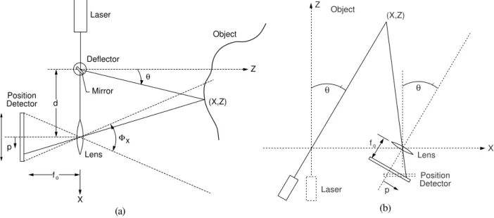
The basic geometrical principle of optical triangulation is shown in Figure 4(a). The light beam generated by the laser is deflected by a mirror and scanned on the object. A camera, composed of a lens and a position sensitive photodetector, measures the location of the image of the illuminated point on the object. By simple trigonometry, the X , Z coordinates of the illuminated point on the object are calculated.

Laser Object Deflector Position Detector P p X Z Lens d Mirror (X,Z) θ Φ_x fo (a) θ θ Object Z Laser Position Detector Lens (X,Z) p X fo (b)

The error in the estimate of Z is inversely proportional to both the separation between the laser and the position detector and the effective position of the lens, but directly proportional to the square of the distance. Unfortunately, f₀ and d cannot be made as large as desired. d is limited mainly by the mechanical structure of the optical setup and by shadow effects.

A synchronized geometry provides a way to alleviate these tradeoffs. Rioux23 introduced a synchronized scanning scheme, with which large fields of view with small triangulation angles can be obtained without sacrificing precision. With smaller triangulation angles, a reduction of shadow effects is inherently achieved. The intent is to synchronize the projection of the laser spot with its detection. As depicted in Figure 4(b), the instantaneous field of view of the position detector, defined by P and f₀, follows the spot as it scans the scene. The focal length of the lens is therefore related to the desired depth of field or measurement range and not to the field of view. Implementation of this triangulation technique by an auto-synchronized scanner approach allows a considerable reduction in the optical head size compared to conventional triangulation methods. Figure 5 displays schematically the basic components of a dual-axis auto-synchronized camera. A 3-D surface map is obtained by (1) scanning a laser beam onto a scene with two oscillating mirrors mounted orthogonally from one another, (2) collecting the light that is scattered by the scene in synchronism with the projection mirrors, and (3) focusing this light onto a linear position detector. See Beraldin et al.20 for the functions of 3-D coordinates computation.

0.5 m _Position Detector Laser Y-Axis Scanner X-Axis Scanner Collecting Lens

Figure 5: Auto-synchronized scanner approach: dual-axis synchronized scanner.

Range cameras based on structured light can generate complete image data of visible surfaces that are rather featureless to the human eye or a video camera. Those that use a laser source can attain depth of fields larger than what is achievable with incoherent light but at the expense of reduced depth precision due to speckle noise. One exception is in the case of synchronized range cameras equipped with a discrete response position detector. These can perform quite well in the presence of speckle noise.24 But unfortunately, range cameras based on structured light methods may produce erroneous results when sudden changes in surface height occur, on surfaces with large reflectance variations and on rough surfaces. This is explained by the fact that, in practice, the laser ray projected onto a scene is not infinitesimal in diameter. Hence, when the laser spot crosses a transition, as shown on Figure 6, the imaged spot will lose most of its symmetry. As the laser spot crosses the reflectance transition, the centroid of the light distribution will shift to indicate, for example, longer distances between the camera and the object being inspected. The result is a small height bump in the range map near the transition. Similarly, when a height step is crossed, the laser spot on the position detector will provide erroneous range data.

S can direction L aser spot

: True centr oid : M easured centroid T rue centroid

Spot distribution on

∆p

Fa r Close

High reflec tance Low reflectance

These conditions are bound to happen in the metrology field because of the many shapes and reflectance characteristics of machined objects. Some systems based upon mirror-like optical arrangements25 or dual-detector arrangements19,26 are capable of eliminating the problems or at least reject erroneous measurements with some basic signal processing. As has been demonstrated in previous work,27 the registered intensity image generated by a regular range camera can be used advantageously to alleviate the impact of erroneous range on edge measurements.

The expected precision from the auto-synchronized laser (ASL) camera measurement at various ranges is shown in figure 7. This curve is computed from the error propagation of measurement of the position of the laser spot on the detector, the scanning mirror controller and the geometry of the sensor.

Distance from camera along Z (m) Expected Precision (mm) 0 0 . 1 0 . 2 0 . 3 0 . 4 0 . 5 0 . 6 0 . 7 0 0 . 5 1 1 . 5 X Y Z

Figure 7: The expected precision of the ASL camera 2.3. BIRIS Technology (Structured Light)

The BIRIS range sensor was developed, at NRC, to work in difficult environments where reliability, robustness, and ease of maintenance are important. The optical principle of BIRIS is shown in Figure 8. The main components are: a mask with two apertures, a camera lens, and a standard CCD camera. In a practical implementation, the double aperture mask replaces the iris of a standard camera lens (hence the name bi-iris). A laser line, produced by a solid state laser diode and a cylindrical lens, is projected on the object and a double image of the line is measured on the CCD camera. The separation between the two imaged lines is proportional to the distance between the object and the camera and provides direct information about the shape and dimensions of the object. For example, in Figure 8, the line separations b1 and b2 represent the ranges Z1 and Z2 respectively. Details of the mathematical model and the calibration can be found in28.

Figure 9 shows accuracy numbers (RMS values of measurements in mm) at various ranges, obtained by BIRIS using 30o field of view with 256 points per profile. The figures were obtained using measurements on planar surfaces at known positions, using a translation stage. It is assumed that laser power and

theoretical referece plane

BIRIS Image Equivalent Range Image

mask Object mathematical transformation b1 b2 from b to z z1 z2 CCD Camera Laser system

Figure 8: The BIRIS range sensor surface reflectance are sufficient to detect the laser line.

Figure 9: Typical accuracy of the BIRIS sensor at various

ranges _{Range [m]} RMS [mm] 0 1 2 3 4 5 6 0 . 3 0 . 6 0 . 9 1 . 2 1 . 5

2.4. The Comparison Criterion

Besl's survey of range sensors29 was intended to provide quantitative comparison of performance between different methods to assist system engineers in performing preliminary evaluation for their applications. He computed a simple figure of merit that combines in a single number: the repeatability or the resolution of measurement (but not the accuracy), speed of data acquisition, and the depth of field. The comparison was based on the data published by the system developers. Here, our criteria for comparing 3-D technologies is based on how accurately the object or the site is recovered. The accuracy (defined in section 4) will be expressed relative to the field of view (FOV). This is the most critical factor that limits the use of a sensor and sometimes is not explicitly provided by the manufacturer. The other criteria for evaluation, such as speed, depth of field, and cost are also important, however, the way they influence the selection criteria is an engineering issue that is beyond the scope of this paper.

3. THE CALIBRATION AND EVALUATION LABORATORY - C E L 3.1. General Description

A laboratory at the Institute for Information Technology of the National Research Council of Canada, has been dedicated to calibration and evaluation of machine vision sensors and systems. Specifically, the objectives of CEL are:

1- Performing precise model-based calibration of various types of sensors and systems and provide internal precision numbers for the sensors.

2- Monitoring sensor stability over time and under variations in environment conditions such as temperature and ambient light.

3- Evaluating system geometric measurement accuracy, with extensive statistical analysis, using a wide range of specially designed standard objects and high- precision positioning devices.

4- Validating computer vision algorithms, such as target and edge measurement, multi-view registration, model-based recognition, and sensor fusion.

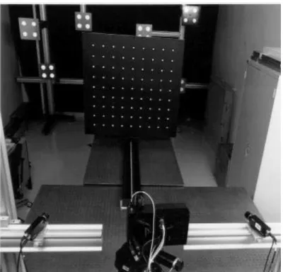
The laboratory (figure 10) is currently equipped with: 1- Precise targets in various arrangements

2- Optical bench, with vibration isolators, and custom mounting devices

3- High precision positioning devices such as translation and rotation stages

4- Theodolites and electronic distance measurement (EDM) devices

5- Standard test objects, of different shapes and sizes, such as planes, spheres, cylinders, and straight and circular edges.

6- PC and SGI workstation. 7- Different light sources.

8- General laboratory equipment such as thermometer, barometer, height gauges, and VCR.

Software tools include, among others;

1- Calibration based on sensor model, including added distortion parameters.

2- Measurement and inspection using 3-D data produced by various types of vision systems (figure 11)

3- Display and manipulation of 3-D data files. 4- Statistical analysis packages.

5- Computer-aided design (CAD).

Figure 10: Part of the CEL showing camera mounts , translation stage and targets

3.2. The Calibration Procedure

The calibration procedure for all the vision sensors in the CEL is described in details in earlier publications.20,27 A plate carrying targets at known locations is imaged by the sensors in at least two positions covering the volume of interest. The positioning of the plate is accomplished by a precise linear stage. The known positions of the targets in the 3-D object space and their extracted position on the sensor are used to solve for the camera parameters, including any modeled distortion parameters. A statistical analysis of the quality of the calibration is also provided to make sure that systematic errors larger than the noise level have been eliminated.

Figure 11: GUI for calibration and measurement software tool

4. TEST PROCEDURE AND RESULTS 4.1. Standards for Performance Tests

ANSI standards for automated vision systems-performance test-measurement of relative position of target features in two dimensional space30, will be followed here, with changes to suit the 3-D space. We will list here some of the definitions from those standards, which will be used in this paper:

Accuracy: The degree of conformance between a measurement of an observable quantity and a recognized standard or specification that indicates the true value of the quantity.

Field of Measurement: The area within which targets or target clusters can be positioned. Field of View: The area of space imaged at the focal plane of a camera.

Repeatability: The degree to which repeated measurements of the same quantity vary about their mean.

Target: A test object or objects having shape, size, position, or relative position characteristics that are known and traceable to recognized standard of measurement.

Test Controller: The computer or other mechanism that initiates the actions, communications with the system under test, and records data necessary for performance of the defined test.

According to the standards, the equipment required for the test are: a machine vision system; a test controller; a target with associated lighting; and a translating table. All these equipment are part of CEL described above. Some of the notable standards are:

● The accuracy of the known target dimensions or relationships between targets shall be at least three times the measured accuracy of the vision system for the test to be valid. This also applies to the accuracy of any translation device.

● At each target location, the machine vision system shall take ten measurements. The number of distinct points measured shall be at least ninety.

● The basic procedure for testing shall be to move the target(s) to a random position and orientation and allow the machine vision system to take measurements. In the standards this procedure is intended for multi-point target plate. For the 3-D test object, we will start with a random position of the object then rotate it by a known angle.

● For multi-point test, the accuracy is calculated by comparing the nominal distance to the measured distance between every pair of points.

We now add one other test procedure:

● For object surfaces and 3-D edges, the accuracy is calculated by comparing the given parameters of the surface or edge-curve function to the computed parameters from fitting the measured data to the function.

The various test objects are shown in figure 12. For the ASL scanner, the field of view used for the reported tests is about 650mmx600mm and the objects are placed at about 800 mm from the camera. All the objects are measured with a coordinate measuring machine (CMM) with better than 0.005 mm accuracy. The ASL-camera accuracy at this range is expected to be about 0.100 mm (figure 7) thus the CMM measurements are well within the standards.

Objects A, B, C and D have known surface parameters while object E, which will be used for edge-measurement tests, has various circular holes of known sizes. The object is placed on a rotating table in order to be positioned at various orientations.

For the ASL and BIRIS cameras, extensive repeatability tests, over several days and at varied temperatures, showed that the data produced are very stable and that the calibration is valid over time. The variations in measurements taken of objects at the same location was at the noise level of the sensor. For the repeatability tests to be realistic, they will also be performed by scanning the objects at different positions and orientation in addition to repeating the measurements at the same position.

4.2. Test Results on Surfaces

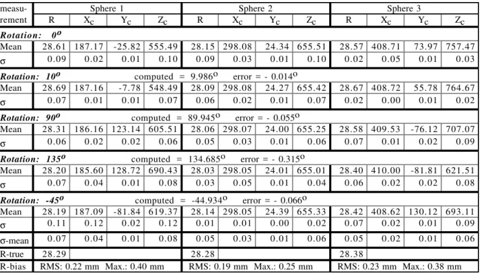
Table 1 displays a sample of the results of measuring object A with the ASL scanner. The object, mounted on a rotating table, was scanned at numerous angular positions. At every position, the X, Y, and Z coordinates of each surface were segmented from the background using a region growing technique. A sphere was fitted to the segmented region using least squares adjustment and the radius and the coordinates of the center of the sphere were determined.

60 0 m m 650 mm 800 mm 0 Camera A B

O bject A : Spheres on a rotating table O bject B : Co ncentric cylinders O bject C: L ong cylinder

O bject D : C om posed of various planes O bject E: Flat object w ith circular holes C D E 1 23 4 1 2 3

Figure 12: Camera set up for evaluation tests and test objects

Object A was designed in such a way so that when it is mounted on the rotating table the center rod axis will coincide with the axis or rotation. The three rods carrying the spheres were placed on a straight line at known distances from each other. Therefore, the computed centers of the spheres can be used to compute the angle of rotation between table positions.

measu- Sphere 1 Sphere 2 Sphere 3

rement R _{Xc Yc Zc} R _{Xc Yc Zc} R _{Xc Yc Zc}

R o t a t i o n : 0 o

Mean 28.61 187.17 -25.82 555.49 28.15 298.08 24.34 655.51 28.57 408.71 73.97 757.47

σ 0.09 0.02 0.01 0.10 0.09 0.03 0.01 0.10 0.02 0.05 0.01 0.03

Rotation: 10o _{computed = 9.986o error = - 0.014o}

Mean 28.69 187.16 -7.78 548.49 28.09 298.08 24.27 655.42 28.67 408.72 55.78 764.67

σ 0.07 0.01 0.01 0.07 0.06 0.02 0.01 0.07 0.02 0.00 0.01 0.02

Rotation: 90o _{computed = 89.945o error = - 0.055o}

Mean 28.31 186.16 123.14 605.51 28.06 298.07 24.00 655.25 28.58 409.53 -76.12 707.07

σ 0.06 0.02 0.02 0.06 0.05 0.03 0.01 0.06 0.07 0.01 0.02 0.09

Rotation: 135o _{computed = 134.685o error = - 0.315o}

Mean 28.20 185.60 128.72 690.43 28.03 298.05 24.01 655.01 28.40 410.00 -81.81 621.51

σ 0.07 0.04 0.01 0.08 0.03 0.05 0.01 0.04 0.06 0.02 0.02 0.08

Rotation: -45o _{computed = -44.934o error = - 0.066o}

Mean 28.19 187.09 -81.84 619.37 28.14 298.05 24.39 655.33 28.42 408.62 130.12 693.11

σ 0.11 0.12 0.02 0.12 0.01 0.01 0.00 0.02 0.07 0.02 0.01 0.09

σ-mean 0.07 0.04 0.01 0.08 0.05 0.03 0.01 0.06 0.05 0.02 0.01 0.06

R-true 28.29 28.28 28.38

R-bias RMS: 0.22 mm Max.: 0.40 mm RMS: 0.19 mm Max.: 0.25 mm RMS: 0.23 mm Max.: 0.38 mm Table 1: Sample results of surface measurements on spheres (R: radius; Xc,Yc,Zc: center)

Table 1 shows the mean of the computed parameters at each position and the standard deviation of the repeated measurements. Tables 2 and 3 display sample results of measurements on cylinders (objects B and C)

Measurement Cyl. B-1 Cyl. B-2 Cyl. B-3 Cyl. B-4 Cyl. C

Radius - mm 39.39 29.81 22.45 12.75 44.25

Axis Angleo 88.41 88.41 88.49 88.39 89.60

True Radius 39.63 30.02 22.60 12.75 44.42

Radius Bias -0.24 -0.21 -0.15 0.00 -0.17

Table 2: Sample results of surface measurements on cylinders (bias)

Measurement # 1 # 2 # 3 # 4 # 5 Mean _σ

Radius - mm 29.86 29.79 29.80 29.83 29.79 29.81 0.03 Axis Angleo 88.54 88.35 88.51 88.43 88.24 88.41 0.11 Table 3: Sample results of repeatability test on cylinder B-2

Plane Surface angle fit-residual RMS angle residualo Plane 1 0 0.139 0 . 0 Plane 2 0 0.132 0.425 Plane 3 2 0 0.121 - 0.273 Plane 4 3 0 0.132 0.124 Plane 5 4 0 0.112 - 0.476 Plane 6 1 0 0.128 0.090

all planes fitting-plane RMS : 0.127 mm surface angle RMS: 0.290 deg. Table 4: Sample results of surface measurements on

planes (object D)

Up to now, the tests dealt with distance measurements. Surface orientation is another issue that can be examined. Because of the ability of range cameras to acquire data from surfaces, one might wonder how well angles between planes can be determined. This question can be answered in two ways. In the first, one tries to predict theoretically the variance of the angle of a plane according to the error propagation model for a range camera, e.g. using the variance-covariance matrix. The model should include random errors, calibration errors and artifact caused by the optical system and the laser spot detection method. Haralick & Shapiro31 present an approximation to the variance of the angle in the case of line fitting where the noise in both coordinates is additive, independent and identically distributed, having zero mean and a distribution that is an even function. They also included the variance-covariance matrix. This error model is of limited use with real range cameras.

The authors are planning to address this issue with a better error model for their range cameras. In the mean time, a second method is recommended. This method is strictly experimental. Hebert et al32. present a more realistic error model for line extraction. They conducted an experiment to estimate the variance-covariance matrix on x and z values as a function of incident angle and depth on an actual range camera. Hence, they achieve invariability in line fitting independently from range camera position. For the purpose of verifying the accuracy and precision in plane extraction, an object with a number of planes was manufactured from a stable material and with tight tolerances. It was then measured with a CMM that is accurate within 25 µm over a distance of 1000 mm. Figure 12 shows a representation of the test object (D). It measures about 250 mm by 250 mm by 100 mm. Table 4 gives the results obtained with a CMM and the ASL camera.

From all the tests on surfaces, the accuracy of the ASL camera, on unmarked surfaces and over a range up to 2.5 m, is about 1:3500 relative to the FOV. For the BIRIS sensor, when similar tests were applied, the accuracy is about 1:2500. 4.3. Test Results on Targets

Target plate mounted on a translation stage (figure 10) was scanned by the camera at various ranges between 500mm and 2500mm. For larger ranges, retroreflective targets mounted on a stable frame at various ranges (shown in figure 10 on the back wall) were employed. The true positions of the targets on the plate were measured with a CMM while those of the targets on the far frame were measured with a theodolite. Both intensity and 3-D data were used to measure the target coordinates with the ASL and the BIRIS cameras. The target center is measured on the intensity image with subpixel accuracy and the corresponding X, Y, and Z coordinates were interpolated from the registered 3-D image. The distances between all the targets were computed and compared to the true distances. Table 5 shows the RMS values of the differences at sample distances using the ASL camera.

distance FOV RMS-X RMS-Y RMS-Z accuracy-XY accuracy-Z

800 650x600 0.080 0.102 0.155 1 : 7200 1 : 4200

2200 1750x1500 0.226 0.235 0.672 1 : 7600 1 : 2600

5600 4500x4100 0.611 0.539 1.950 1 : 7700 1 : 2300

4.4. Test Results on Edges

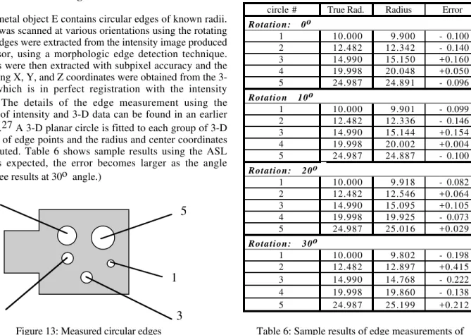
The flat metal object E contains circular edges of known radii. The object was scanned at various orientations using the rotating table. The edges were extracted from the intensity image produced by the sensor, using a morphologic edge detection technique. Edge points were then extracted with subpixel accuracy and the corresponding X, Y, and Z coordinates were obtained from the 3-D image which is in perfect registration with the intensity image.33 The details of the edge measurement using the integration of intensity and 3-D data can be found in an earlier publication.27 A 3-D planar circle is fitted to each group of 3-D coordinates of edge points and the radius and center coordinates were computed. Table 6 shows sample results using the ASL camera. As expected, the error becomes larger as the angle increases (see results at 30o angle.)

4

5

1

3

2

Figure 13: Measured circular edges

circle # True Rad. Radius Error

R o t a t i o n : 0 o 1 10.000 9.900 - 0.100 2 12.482 12.342 - 0.140 3 14.990 15.150 +0.160 4 19.998 20.048 +0.050 5 24.987 24.891 - 0.096 R o t a t i o n 1 0 o 1 10.000 9.901 - 0.099 2 12.482 12.336 - 0.146 3 14.990 15.144 +0.154 4 19.998 20.002 +0.004 5 24.987 24.887 - 0.100 R o t a t i o n : 2 0 o 1 10.000 9.918 - 0.082 2 12.482 12.546 +0.064 3 14.990 15.095 +0.105 4 19.998 19.925 - 0.073 5 24.987 25.016 +0.029 R o t a t i o n : 3 0 o 1 10.000 9.802 - 0.198 2 12.482 12.897 +0.415 3 14.990 14.768 - 0.222 4 19.998 19.860 - 0.138 5 24.987 25.199 +0.212

Table 6: Sample results of edge measurements of circles

The accuracy on edges obtained from all the tests translates to about 1:7500 of the FOV (excluding edges at 30o angles and larger.) For the BIRIS sensor, similar tests were performed and the resulting accuracy was about 1:1500.

5. CONCLUDING REMARKS

We briefly presented an approach to evaluating the measurement accuracy of machine vision systems. The procedure can be applied to passive and active systems. A specially equipped calibration and evaluation laboratory has been used to evaluate the 3-D vision systems developed at the National Research Council of Canada. Results from the active systems have been presented and a comparison with passive vision systems employing photogrammetric principals is as follows:

1- On well defined targets, the accuracy obtained by active systems is much lower than the one obtained by a photogrammetric system (1: 3000 - 1:7500 for the ASL scanner compared to 1:20000 or better). Therefore, for applications allowing the placement of targets on the object surfaces and requiring high accuracy, passive systems are the obvious choice.

2- On edges, passive systems still provide better accuracy than active systems (1:15,000 or better compared to 1:7500 for the ASL scanner). It should be noted, however, that the active systems provide a more complete 3-D data on all the visible edges in the scene while the passive system will be affected significantly by the ambient light and may require several camera arrangements to extract 3-D coordinates on all edges. Therefore, the choice here is not as obvious as in the case of targets and is dependent on the application environment particularly since the accuracy from an active system, particularly the ASL camera, may be acceptable for many applications.

3- On untargeted surfaces, active systems can provide a complete 3-D map of the visible surfaces with about 1:3500 accuracy while passive systems may not be able to acquire any measurements without distinguished features. Therefore, the comparison based on accuracy is not valid here.

From the above short comparison, selection of a vision technology is largely dependent on the type of feature to be measured and the required accuracy. In some applications, when a variety of features are required to be measured, a combination of different technologies may be the answer. The results presented in this paper are intended to help system engineers in making the choice.

REFERENCES

1. S. Yi, R.M. Haralick and L.G. Shapiro, "Error propagation in machine vision", Machine Vision and Applications, 7 (2), 93-114, 1994.

2. H.A. Beyer, T.Kersten, and A.Streilein,"Metric accuracy performance of solid-state camera systems", in Proc.

Videometrics, SPIE-1820, 103-110, 1992.

3. P.C. Gustafson, "An accuracy / repeatability test for a video photogrammetric measurement", in Proc. Industrial Vision

Metrology, SPIE-1526, 36-41, 1991.

4. C.S. Fraser, and M.R.Shortis,"Vision metrology in industrial inspection: a practical evaluation", International Archives

of Photogrammetry and Remote Sensing, XXX (5); 87-91, 1994.

5. H.-G. Maas and T.P. Kersten, "Experiences with a high resolution still video camera in digital photogrammetric applications on a shipyard", International Archives of Photogrammetry and Remote Sensing, XXX (5); 250-255, 1994.

6. J. Peipe, C.-T. Schneider and K. Sinnreich,"Performance of a PC based digital photogrammetric station", International

Archives of Photogrammetry and Remote Sensing, XXX (5); 304-309, 1994.

7. S.F. El-Hakim,"Application and performance evaluation of a vision-based automated measurement system", in Proc.

Videometrics, SPIE-1820, 181-195, 1992.

8. A. Gruen and D. Stallmann, "High accuracy matching of object edges", in Proc. Videometrics, SPIE-1820, 70-82, 1992.

9. J. Dahler, "Problems in digital image acquisition with CCD cameras," ISPRS Intercommission conference on fast processing of photogrammetric data, pp. 48-59, 1987.

10. Lenz, R. and D.Fritsch,“On the accuracy of videometry”, International Archives of Photogrammetry and Remote Sensing, XXVII (B5); 345-355, 1988.

11. H.A. Beyer, "Some aspects of the geometric calibration of CCD-cameras", ISPRS Intercommission Conference on fast processing of photogrammetric data, Interlaken, 1987.

12. T. Luhmann and W.Wester-Ebbinghaus, "On geometric calibration of digital video images of CCD arrays", ISPRS Intercommission conference on fast processing of photogrammetric data, Interlaken, 1987.

13. D.T. Havelock, “Geometric precision in noise-free digital images,” IEEE Trans. Pattern Analysis and Machine

Intelligence, PAMI-11(10), 1065-1075, 1989.

14. J.D. Thurgood and E.M. Mikhail, "Subpixel mensuration of photogrammetric targets in digital images", School of Civil Engineering, Purdue University, Tech. Report CE-PH-82-2, (1982.

15.R.O. Mitchell, E.P. Lyvers, K.A. Dunkelberger and M.L.Akey, "Recent results in precision measurements of edges, angles, areas and perimeters", SPIE Vol. 730, Automated Inspection and Measurement, pp. 123-134, 1986.

16. Fraser, C.S., “Network design considerations for non-topographic photogrammetry”, Photogrammetric Engineering and Remote Sensing, 50(8); 1115-1126, 1994.

17. Fraser, C.S.,"Limiting error propagation in network design", Photogrammetric Engineering and Remote Sensing, 53(5); 487-493, 1987.

18. P.J. Besl,”Active, optical range imaging sensors”, Machine Vision and Applications, 1(2), 127-152, 1988.

19. M. Buzinski, A. Levine and W.H. Stevenson,"Performance characteristics of range sensors utilizing optical triangulation", in IEEE/AESS National Aerospace and Electronics Conference Proc., 1230-1236, 1992.

20. J.-A. Beraldin, S.F. El-Hakim and L. Cournoyer,”Practical range camera calibration”, in Proc.Videometrics II, SPIE 2067, 21-31, 1993.

21. J. Paakkari and I. Moring, "Method for evaluating the performance of range imaging devices", in Proc. Industrial Applications of Optical Inspection, Metrology, and Sensing", SPIE 1821, 350-356, 1992.

22. D. Petkovic, B. Dom, J. Sanz, and J. Mandville, "Verifying accuracy of machine vision algorithms and systems", in Proc. 22nd ASILOMAR Conf. Signals, Systems and Computers, MAPLE Press, 955-961, 1988.

23. M. Rioux, ”Laser range finder based on synchronized scanners”, Applied Optics, 23, 3837-3844 (1984).

24. R. Baribeau and M. Rioux,"Influence of speckle on laser range finders", Applied Optics, 30, 2873--2878 (1991). 25. F. Blais, M. Rioux and J. Domey,"Optical range image acquisition for the navigation of a mobile robot", in Proc.

IEEE Intl. Conf. Robotics and Automation, Sacrameto, Apr. 9-11, 2574-2580 (1991).

26. K.S. Kooijman and J.L. Horijon,"Video rate laser scanner: Considerations on triangulation optics, detectors and processing circuits", in Optics, Illumination, and Image Sensing for Machine Vision VIII, Proc. SPIE 2065, 251-263 (1993).

27. S.F. El-Hakim and J.-A. Beraldin,"On the integration of range and intensity data to improve vision-based three-dimensional measurements", in Videometrics III, Proc. SPIE 2350, 306-321, 1994.

28. Blais, F., M.Lecavalier, J.Domey, P.Boulanger, and J.Courteau,"Application of the BIRIS range sensor for wood volume measurement", NRC/ERB-1038, 19 pages, 1992.

29. P.J. Besl, "Range imaging sensors", General Motors Research Publication GMR-6090, Warren, Michigan, 1988. 30. American National Standard for Automated Vision Systems - Performance Test - Measurement of Relative Position of

Target Features in Two-Dimensional Space. ANSI/AVA A15.05/1 - 1989.

31. R.M. Haralick and L.G. Shapiro, "Computer and Robot Vision", Chap. 11 Arc Extraction and Segmentation, Addison-Wesley Publishing Company, 1992.

32. P. Hebert, D. Laurendeau and D. Poussart, "Surface Profile Description: Invariant Stable Extraction of Straight Line Segments", Vision Interface 93, Toronto, Canada, pp.21-26, 1993.

33. J.-A.Beraldin, M.Rioux, F.Blais, L.Cournoyer and J.Domey, ”Registered intensity and range imaging at 10 mega-samples per second,” Optical Engineering, 31(1), 88-94, (1992).