HAL Id: hal-01373784
https://hal.archives-ouvertes.fr/hal-01373784
Submitted on 29 Sep 2016
HAL is a multi-disciplinary open access
archive for the deposit and dissemination of
sci-entific research documents, whether they are
pub-lished or not. The documents may come from
teaching and research institutions in France or
abroad, or from public or private research centers.
L’archive ouverte pluridisciplinaire HAL, est
destinée au dépôt et à la diffusion de documents
scientifiques de niveau recherche, publiés ou non,
émanant des établissements d’enseignement et de
recherche français ou étrangers, des laboratoires
publics ou privés.
Fast Single Image Super-Resolution Using a New
Analytical Solution for l2–l2 Problems
Ningning Zhao, Qi Wei, Adrian Basarab, Nicolas Dobigeon, Denis Kouamé,
Jean-Yves Tourneret
To cite this version:
Ningning Zhao, Qi Wei, Adrian Basarab, Nicolas Dobigeon, Denis Kouamé, et al.. Fast Single Image
Super-Resolution Using a New Analytical Solution for l2–l2 Problems. IEEE Transactions on Image
Processing, Institute of Electrical and Electronics Engineers, 2016, vol. 25 (n° 8), pp. 3683-3697.
�10.1109/TIP.2016.2567075�. �hal-01373784�
O
pen
A
rchive
T
OULOUSE
A
rchive
O
uverte (
OATAO
)
OATAO is an open access repository that collects the work of Toulouse researchers and
makes it freely available over the web where possible.
This is an author-deposited version published in :
http://oatao.univ-toulouse.fr/
Eprints ID : 16140
To link to this article : DOI : 10.1109/TIP.2016.2567075
URL :
http://dx.doi.org/10.1109/TIP.2016.2567075
To cite this version :
Zhao, Ningning and Wei, Qi and Basarab,
Adrian and Dobigeon, Nicolas and Kouamé, Denis and Tourneret,
Jean-Yves Fast Single Image Super-Resolution Using a New
Analytical Solution for l2–l2 Problems. (2016) IEEE Transactions
on Image Processing, vol. 25 (n° 8). pp. 3683-3697. ISSN
1057-7149
Any correspondence concerning this service should be sent to the repository
administrator:
[email protected]
Fast Single Image Super-Resolution Using a New
Analytical Solution for ℓ
2
–ℓ
2
Problems
Ningning Zhao, Student Member, IEEE, Qi Wei, Student Member, IEEE, Adrian Basarab, Member, IEEE,
Nicolas Dobigeon, Senior Member, IEEE, Denis Kouamé, Member, IEEE,
and Jean-Yves Tourneret, Senior Member, IEEE
Abstract— This paper addresses the problem of single image super-resolution (SR), which consists of recovering a high-resolution image from its blurred, decimated, and noisy version. The existing algorithms for single image SR use different strate-gies to handle the decimation and blurring operators. In addition to the traditional first-order gradient methods, recent techniques investigate splitting-based methods dividing the SR problem into up-sampling and deconvolution steps that can be easily solved. Instead of following this splitting strategy, we propose to deal with the decimation and blurring operators simultaneously by taking advantage of their particular properties in the frequency domain, leading to a new fast SR approach. Specifically, an analytical solution is derived and implemented efficiently for the Gaussian prior or any other regularization that can be formulated into an ℓ2-regularized quadratic model, i.e., an ℓ2–ℓ2 optimization
problem. The flexibility of the proposed SR scheme is shown through the use of various priors/regularizations, ranging from generic image priors to learning-based approaches. In the case of non-Gaussian priors, we show how the analytical solution derived from the Gaussian case can be embedded into traditional splitting frameworks, allowing the computation cost of existing algorithms to be decreased significantly. Simulation results conducted on several images with different priors illustrate the effectiveness of our fast SR approach compared with existing techniques.
Index Terms— Single image super-resolution, deconvolution, decimation, block circulant matrix, variable splitting based algorithms.
I. INTRODUCTION
S
INGLE image super-resolution (SR), also known as image scaling up or image enhancement, aims at estimating a high-resolution (HR) image from a low-resolution (LR) observed image [1]. This resolution enhancement problem is still an ongoing research problem with applications in variousN. Zhao, N. Dobigeon, and J.-Y. Tourneret are with the Univer-sity of Toulouse, Toulouse 31071, France (e-mail: [email protected]; [email protected]; [email protected]).
Q. Wei is with the Department of Engineering, University of Cambridge, Cambridge CB21PZ, U.K. (e-mail: [email protected]).
A. Basarab and D. Kouamé are with the Institut de Recherche en Informa-tique de Toulouse, University of Toulouse, Toulouse F-31062, France (e-mail: [email protected]; [email protected]).
Digital Object Identifier 10.1109/TIP.2016.2567075
fields, based on remote sensing [2], video surveillance [3], hyperspectral [4], microwave [5] or medical imaging [6].
The methods dedicated to single image SR can be classi-fied into three categories [7]–[9]. The first category includes the interpolation based algorithms based on nearest neighbor interpolation, bicubic interpolation [10] or adaptive inter-polation techniques [11], [12]. Despite their simplicity and easy implementation, it is well-known that these algorithms generally over-smooth the high frequency details. The second type of methods consider learning-based (or example-based) algorithms that learn the relations between LR and HR image patches from a given database [7], [13]–[16]. Note that the effectiveness of the learning-based algorithms highly depends on the training image database and that these algorithms have generally a high computational complexity. Reconstruction-based approaches that are considered in this paper belong to the third category of SR approaches [8], [9], [17], [18]. These approaches formulate the image SR as a reconstruction prob-lem, either by incorporating priors in a Bayesian framework or by introducing regularizations into an inverse problem.
Existing reconstruction-based techniques used to solve the single image SR include the first order gradient-based meth-ods [7]–[9], [17], the iterative shrinkage thresholding-based algorithms [19] (also called forward-backward algorithms), proximal gradient algorithms and other variable splitting algo-rithms that rely on the augmented Lagrangian (AL) scheme. The AL-based algorithms include the alternating direction method of multipliers (ADMM) [2], [6], [18], [20], split Bregman (SB) methods [5] (known to be equivalent to ADMM in certain conditions [21]) and their variants. Particularly, Ng
et al. [18] proposed an ADMM-based algorithm to solve a
TV-regularized single image SR problem, where the decima-tion and blurring operators are split and solved iteratively. Due to this splitting, the cumbersome SR problem can be decomposed into an up-sampling problem and a deconvolution problem, that can be both solved efficiently. Yanovsky et
al. [5] proposed to solve the same problem with an Split
Bregman (SB) algorithm. However, the decimation operator was handled through a gradient descent method integrated in the SB framework. Sun et al. [8], [17] proposed a gradient profile prior and formulated the single image SR problem as an ℓ2-regularized optimization problem, further solved with the gradient descent method. Yang et al. [7] proposed a learning-based algorithm for single image SR by seek-ing a sparse representation usseek-ing the patches of LR and
HR images, followed by back-projection through a gradient descent method.
This paper aims at reducing the computational cost of these SR methods by proposing a new approach handling the decimation and blurring operators simultaneously by explor-ing their intrinsic properties in the frequency domain. It is interesting to note that similar properties were explored in [22] and [23] for multi-frame SR. However, the implemen-tation of the matrix inversions proposed in [22] and [23] are less efficient than those proposed in this work, as it will be demonstrated in the complexity analysis conducted in Section III. More precisely, this paper derives a closed-form expression of the solution associated with the ℓ2-penalized least-squares
SR problem, when the observed LR image is assumed to be a noisy, subsampled and blurred version of the HR image with a spatially invariant blur. This model, referred to as ℓ2–ℓ2in
what follows, underlies the restoration of an image contami-nated by additive Gaussian noise and has been used intensively for the single image SR problem, see, e.g., [7], [8], [24]. The proposed solution is shown to be easily embeddable into an AL framework to handle non-Gaussian priors (i.e., non-ℓ2
regularizations), which significantly lightens the computational burdens of several existing SR algorithms.
The remainder of the paper is organized as follows. Section II formulates the single image SR problem as an optimization problem. In Section III, we study the properties of the down-sampling and blurring operators in the frequency domain and introduce a fast SR scheme based on an ana-lytical solution for the ℓ2–ℓ2 model that can be formulated
in the image or gradient domains. Section IV generalizes the proposed fast SR scheme to more complex regularizations in image or transformed domains. Various experiments presented in Section V demonstrate the efficiency of the proposed fast single image SR scheme. Conclusions and perspectives are finally reported in Section VI.
II. IMAGESUPER-RESOLUTIONFORMULATION
A. Model of Image Formation
In the single image SR problem, the observed LR image is modeled as a noisy version of the blurred and decimated HR image to be estimated as follows,
y = SHx + n (1)
where the vector y ∈ RNl×1(N
l = ml × nl) denotes the LR
observed image and x ∈ RNh×1(N
h = mh × nh) is the
vectorized HR image to be estimated, with Nh > Nl. The
vectors y and x are obtained by stacking the corresponding images (LR image ∈ Rml×nl and HR image ∈ Rmh×nh) into
column vectors in a lexicographic order. Note that the vector
n ∈ RNl×1 is an independent identically distributed (i.i.d.)
additive white Gaussian noise (AWGN) and that the matrices
S ∈ RNl×Nh and H ∈ RNh×Nh represent the decimation
and the blurring/convolution operations respectively. More specifically, H is a block circulant matrix with circulant blocks, which corresponds to cyclic convolution boundaries, and left multiplying by S performs down-sampling with an integer factor d (d = dr × dc), i.e., Nh = Nl × d. The decimation
factors dr and dc represent the numbers of discarded rows
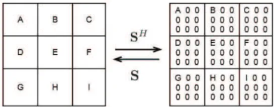
Fig. 1. Effect of the up-sampling matrix SH on a 3 × 3 image and of the
down-sampling matrix S on the corresponding 9 × 9 image (whose scale up factor equals 3).
and columns from the input images satisfying the following relationships mh = ml × dr and nh = nl × dc. Note that
the image formation model (1) has been widely considered in single image SR problems, see, e.g., [7], [8], [17], [18], [25]. We introduce two additional basic assumptions about the blurring and decimation operators. These assumptions have been widely used for image deconvolution or image SR problems (see, e.g., [7], [16], [26], [27]) and are necessary for the proposed fast SR framework.
Assumption 1: The blurring matrix H is the matrix repre-sentation of the cyclic convolution operator, i.e., H is a block circulant matrix with circulant blocks (BCCB).
This assumption has been widely used in the image process-ing literature [22], [23], [28]. It is satisfied provided the blur-ring kernel is shift-invariant and the boundary conditions make the convolution operator periodic. Note that the BCCB matrix assumption does not depend on the shape of the blurring kernel, i.e., it is satisfied for any kind of blurring, including motion blur, out-of-focus blur, atmospheric turbulence, etc. Using the cyclic convolution assumption, the blurring matrix and its conjugate transpose can be decomposed as
H = FH3F (2)
HH = FH3HF (3) where the matrices F and FH are associated with the Fourier
and inverse Fourier transforms (satisfying FFH = FHF = I Nh)
and 3 = diag{Fh} ∈ CNh×Nh is a diagonal matrix, whose
diagonal elements are the Fourier coefficients of the first column of the blurring matrix H, denoted as h. Using the decompositions (2) and (3), the blurring operator Hx and its conjugate HHx can be efficiently computed in the frequency
domain, see, e.g., [26], [29], [30].
Assumption 2: The decimation matrix S ∈ RNl×Nh is a
down-sampling operator, while its conjugate transpose SH ∈ RNh×Nl interpolates the decimated image with zeros.
Once again, numerous research works have used this assumption [7], [16], [22], [23]. Fig. 1 shows a toy example highlighting the roles of the decimation matrix S and its conjugate transpose SH. The decimation matrix satisfies the
relationship SSH = I
Nl. Denoting S , S
HS, multiplying
an image by S can be achieved by making an entry-wise multiplication with an Nh × Nh mask having ones at the
sampled positions and zeros elsewhere.
B. Problem Formulation
Similar to traditional image reconstruction problems, the estimation of an HR image from the observation of an
LR image is not invertible, leading to an ill-posed problem. This ill-posedness is classically overcome by incorporating some appropriate prior information or regularization term. The regularization term can be chosen from a specific task of interest, the information resulting from previous experi-ments or from a perceptual view on the constraints affecting the unknown model parameters [31], [32]. Various priors or regularizations have already been advocated to regular-ize the image SR problem include: (i) traditional generic image priors such as Tikhonov [24], [33], [34], the total variation (TV) [18], [20], [35] and the sparsity in trans-formed domains [36]–[39], (ii) more recently proposed image regularizations such as the gradient profile prior [8], [9], [17] or Fattal’s edge statistics [40] and (iii) learning-based priors [41], [42]. The fast approach proposed in the next section is shown to be adapted to many of the existing regularization terms. Note that proposing new regularization terms with improved SR performance is out of the scope of this paper.
Assuming that the noise n in (1) is AWGN and incorporat-ing a proper regularization to the target image x, the maximum
a posteriori(MAP) estimator of x for the single image SR can
be obtained by solving the following optimization problem min x 1 2ky − SHxk 2 2 ! "# $ data fidelity + τ φ(Ax) ! "# $ regularization (4) where ky − SHxk2
2 is a data fidelity term associated with
the model likelihood and φ(Ax) is related to the image prior information and is referred to as regularization or penalty [43]. Note that the matrix A can be the identity matrix when the regularization is imposed on the SR image itself, the gradient operator, any orthogonal matrix or normalized tight frame, depending on the addressed application and the properties of the target image. The role of the regularization parameter τ is to weight the importance of the regularization term with respect to (w.r.t.) the data fidelity term. The next section derives a closed-form solution of the problem (4) for a quadratic regularizing operator φ(·) when the assumptions 1 and 2 hold.
III. PROPOSEDFASTSUPER-RESOLUTION
USING ANℓ2-REGULARIZATION
Before proceeding to more complicated regularizations investigated in Section IV, we first consider the basic ℓ2-norm regularization defined by
φ(Ax) = kAx − vk22 (5) where the matrix AHAis assumed, unless otherwise specified,
to be invertible. Typical examples of matrices A include the Fourier transform matrix, the wavelet transform matrix, etc. Under this ℓ2-norm regularization, a generic form of a fast solution to problem (4) will be derived in Section III-A. Then, two particular cases of this regularization widely used in the literature will be discussed in Sections III-B and III-C.
A. Proposed Closed-Form Solution for theℓ2–ℓ2Problem
With the regularization (5), the problem (4) transforms to min
x 1
2ky − SHxk22+ τ kAx − vk22 (6) whose solution is given by
ˆx = (HHSH +2τ AHA)−1(HHSHy +2τ AHv) (7)
with S = SHS. Direct computation of the analytical solution
(7) requires the inversion of a high dimensional matrix, whose computational complexity is of order O(N3
h). One can think of
using optimization or simulation-based methods to overcome this computational difficulty. The optimization-based methods, such as the gradient-based methods [17] or, more recently, the ADMM [18] and SB [5] method approximate the solution of (6) by iterative updates. The simulation-based methods, e.g., the Markov Chain Monte Carlo methods [44]–[46], are drawing samples from a multivariate posterior distribution (which is Gaussian for a Tikhonov regularization) and compute the average of the generated samples to approximate the minimum mean square error (MMSE) estimator of x. However, simulation-based methods have the major drawback of being computationally expensive, which prevents their effective use when processing large images. Moreover, because of the particular structure of the decimation matrix, the joint operator
SH cannot be diagonalized in the frequency domain, which prevents any direct implementation of the solution (7) in this domain. The main contribution of this work is to propose a new scheme to compute (7) explicitly, getting rid of any sampling or iterative update and leading to a fast SR method. In order to compute the analytical solution (7), a property of the decimation matrix in the frequency domain is first stated in Lemma 1.
Lemma 1 (Wei et al. [34]): The following equality holds
FSFH = 1
dJd⊗ INl (8)
where Jd ∈ Rd×d is a matrix of ones, INl ∈ R
Nl×Nl is the
Nl× Nl identity matrix and ⊗ is the Kronecker product.
Using the property of the matrix FSFH given in Lemma 1
and taking into account the assumptions mentioned above, the analytical solution (7) can be rewritten as
ˆx = FH% 1 d3 H3+2τ FAHAFH &−1 F'HHSHy +2τ AHv( (9) where the matrix 3 ∈ CNl×Nh is defined as
3= [31, 32, · · · , 3d] (10)
and where the blocks 3i ∈ CNl×Nl (i = 1, · · · , d) satisfy the
relationship
diag{31, · · · , 3d} = 3. (11)
The readers may refer to the Appendix A for more details about the derivation of (9) from (7).
To further simply the expression (9), we propose to use the following Woodbury inverse formula.
Lemma 2 (Woodbury Formula [47]): The following equal-ity holds conditional on the existence of A−11 and A−13
(A1+ A2A3A4)−1
= A−11− A−11A2(A−31+ A4A−11A2)−1A4A−11 (12)
where A1, A2, A3 and A4 are matrices of correct sizes.
Taking into account the Woodbury formula of Lemma 2, the analytical solution (9) can be computed very efficiently as stated in the following theorem.
Theorem 1: When Assumptions 1 and 2 are satisfied, the solution of Problem (6) can be computed using the following closed-form expression ˆx = 1 2τF H9Fr − 1 2τF H93H)2τ dI Nl + 393 H*−139Fr (13) where r = HHSHy +2τ AHv, 9 = F'AHA(−1FH and 3 is defined in (10).
Proof: See Appendix A.
Complexity Analysis: The most computationally expensive
part for the computation of (13) in Theorem 1 is the imple-mentation of FFT/iFFT. In total, four FFT/iFFT computations are required in our implementation. Comparing with the original problem (7), the order of computation complexity has decreased significantly from O(Nh3) to O(Nhlog Nh),
which allows the analytical solution (13) to be computed efficiently. Note that [22] and [23] also addressed image SR problems by using the properties of S in the frequency domain, where Nl small matrices of size d × d were inverted. The
total computational complexity of the methods investigated in [22] and [23] is O(Nhlog Nh+ Nhd2). Another important
difference with our work is that the authors of [22] and [23] decomposed the SR problem into an upsampling (including motion estimation which is not considered in this work) and a deblurring step. The operators H and S were thus considered separately, thus requiring two ℓ2regularizations for the blurred
image (referred to as z in [22]) and the ground-truth image (referred to as x in [22]). On the contrary, this work considers the blurring and downsampling jointly and achieve the SR in one step, requiring only one regularization term for the unknown image. It is worthy to mention that the proposed SR solution can be extended to incorporate the warping operator considered in [22] and [23], which can also be modelled as a BCCB matrix. This is not included in this paper but will be considered in future work.
In the sequel of this section, two particular instances of the ℓ2-norm regularization are considered, defined in the image
and gradient domains, respectively.
B. Solution of the ℓ2–ℓ2 Problem in the Image Domain
First, we consider the specific case where A = INh and v = ¯x, i.e., the problem (6) turns to
min x 1 2ky − SHxk 2 2+ τ kx − ¯xk22. (14)
This implies that the target image x is a priori close to the image ¯x. The image ¯x can be an estimation of the HR image,
Algorithm 1 FSR With Image-Domain ℓ2-Regularization:
Implementation of the Analytical Solution (15)
e.g., an interpolated version of the observed image, a restored image obtained with learning-based algorithms [7] or a cleaner image obtained from other sensors [24], [34], [48]. In such case, using Theorem 1, the solution of the problem (14) is
ˆx = 1 2τr − 1 2τF H3H)2τ dI Nl + 33 H*−13Fr (15) with r = HHSHy +2τ ¯x.
Algorithm 1 summarizes the implementation of the pro-posed SR solution (15), which is referred to as fast
super-resolution (FSR)approach.
C. Solution of theℓ2–ℓ2 Problem in the Gradient Domain
Generic image priors defined in the gradient domain have been successfully used for image reconstruction, avoiding the common ringing artifacts see, e.g., [8], [9], [17]. In this part, we focus on the gradient profile prior proposed in [17] for the single image SR problem. This prior consists of considering the regularizing term k∇x − ¯∇xk22, yielding the following problem
min x
1
2ky − SHxk22+ τ k∇x − ¯∇xk22 (16) where ∇ is the discrete version of the gradient ∇ := [∂h, ∂v]T
and ¯∇x is the estimated gradient field. More explanations about the motivations for using the gradient field may be found in [8] and [17]. For an image x ∈ Rm×n, under the periodic
boundary conditions, the numerical definitions of the gradient operators are
(∂hx)(i, j ) = x((i +1) mod m, j) − x(i, j) if i ≤ m (∂vx)(i, j ) = x(i, ( j +1) mod n) − x(i, j) if j ≤ n
where ∂hand ∂vare the horizontal and vertical gradients. The gradient operators can be rewritten as two BCCB matrices Dh and Dv corresponding to the horizontal and vertical discrete
Algorithm 2 FSR With Gradient-Domain ℓ2-Regularization:
Implementation of the Analytical Solution of (16)
matrices 6h and 6v (CNh×Nh) are obtained by decomposing Dh and Dvin the frequency domain, i.e.,
Dh= FH6hF and Dv= FH6vF. (17) Thus, the problem (16) can be transformed into
min x 1 2ky − SHxk 2 2+ τ kAx − vk22 (18) with A = [DT
h, DTv] ∈ R2Nh×Nh and using the notation ¯∇x = v = [vh, vv]T ∈ R2Nh×1. Note that the invertibility of AHA
is violated here because of the periodic boundary assumption. Thus, adding a small ℓ2-norm regularization τ σ kxk2
2 (where
σ is a very small constant) to (18) can circumvent this invertibility problem while keeping the solution close to the original regularization. Using Theorem 1, the analytical solu-tion of (18) (including the addisolu-tional small ℓ2-norm term) is
given by (13) with 9 ='6hH6h+ 6vH6v+ σ IN
h
(−1 . The pseudocode used to implement this solution is summa-rized in Algo. 2.
IV. GENERALIZEDFASTSUPER-RESOLUTION
As mentioned previously, a large variety of non-Gaussian regularizations have been proposed for the single image SR problem, in both image or transformed domains. Many SR algorithms, e.g., [5], [18], require to solve an ℓ2–ℓ2 problem
similar to (6) as an intermediate step. This section shows that the solution (13) derived in Section III can be combined with existing SR iterative methods to significantly lighten their computational costs.
A. General Form of the Proposed Algorithm
In order to use the analytical solution (13) derived for the ℓ2-regularized SR problem into an ADMM framework,
Algorithm 3 Proposed Generalized Fast Super-Resolution
(FSR) Scheme
the problem (4) is rewritten as the following constrained optimization problem min x,u 1 2ky − SHxk 2 2+ τ φ(u) subject to Ax = u. (19) The AL function associated with this problem is
L(x, u, λ) = 1 2ky − SHuk 2 2+ τ φ(u) + λT(Ax − u) + µ 2kAx − uk 2 2 or equivalently L(x, u, d) = 1 2ky − SHuk22+ τ φ(u) + µ 2kAx − u + dk22. (20) To solve problem (19), we need to minimize L(x, u, d) w.r.t.
x and u and update the scaled dual variable d iteratively as
summarized in Algo. 3.
Note that the 3rd step updating the HR image x can be solved analytically using Theorem 1. The variable u is updated at the 4th step using the Moreau proximity operator whose definition is given by proxλ,φ(ν) =argmin x φ(x) + 1 2λkx − νk 2. (21)
The generic optimization scheme given in Algo. 3, including the non-iterative update of the HR image following Theo-rem 1, is detailed hereafter for three widely used regularization techniques, namely the TV regularization [18], the ℓ1-norm regularization in the wavelet domain [38] and the learning-based method of [7].
B. TV Regularization
Using a TV prior, problem (4) can be rewritten as min
x 1
2ky − SHxk22+ τ φ(Ax) (22) where the regularization term is given by
φ(Ax) = kxkTV =
+
kDhxk2+ kDvxk2 (23)
with A = [Dh, Dv]T ∈ R2Nh×Nh. We can solve (22) using
Algo. 3, with the auxiliary variable u = [uh, uv]T ∈ R2Nh×1
such that Ax = u. The resulting pseudocodes of the proposed fast SR approach for solving (22) are detailed in Algo. 4, which is reported in Appendix B.
C. ℓ1-Norm Regularization in the Wavelet Domain
Assuming that x can be decomposed as a linear combination of wavelets (e.g., as in [36]), the SR can be conducted in the wavelet domain. Denote as x = Wθ the wavelet decomposition of x, where θ ∈ RNh×1is the vector containing
the wavelet coefficients and multiplying by the matrices WH
and W (∈ RNh×Nh) represent the wavelet and inverse wavelet
transforms (satisfying that WWH = WHW = I
Nh). The
single image SR with ℓ1-norm regularization in the wavelet
domain can be formulated as follows min x 1 2ky − SHxk 2 2+ τ kAxk1 (24)
where A = WH. By introducing the additional variable
u = WHx, the problem (24) can be solved using Algo. 3. The
corresponding pseudocodes of the resulting fast SR algorithm with an ℓ1-norm regularization in the wavelet domain are detailed in Algo. 5 in Appendix B.
D. Learning-Basedℓ2-Norm Regularization
The effectiveness of the learning-based regularization for image reconstruction has been proved in several studies. In particular, Yang et al. [7] solved the single image SR problem by jointly training two dictionaries for the LR and HR image patches and by applying sparse coding (SC). Interestingly, the HR image x0obtained by SC was projected
onto the solution space satisfying (1), leading to the following optimization problem ˆx =argmin x 1 2ky − SHxk 2 2+ τ kx − x0k22. (25)
This optimization problem was solved using a gradient descent approach in [7]. However, it can benefit from the analytical solution provided by Theorem 1 that can be implemented using Algo. 1.
V. EXPERIMENTALRESULTS
This section demonstrates the efficiency of the proposed fast SR strategy by testing it on various images with different regularization terms. The performance of the single image SR algorithms is evaluated in terms of reconstruction quality and computational load. Given the ability of our algorithm to solve the SR problem with less complexity than the existing methods, one may expect a gain in computational time and convergence properties. All the experiments were performed using MATLAB 2013A on a computer with Windows 7, Intel(R) Core(TM) i7-4770 CPU @3.40GHz and 8 GB RAM.1
Color images were processed using the illuminate channel only, as in [7]. Precisely, the RGB images were transformed into YUV coordinates and the color channels (Cb,Cr) were up-sampled using bicubic interpolation. In the illuminate channel, the HR image was blurred and down-sampled in each spatial direction with factors dr and dc. The resulting blurred and
1The MATLAB codes are available in the first author’s homepage
http://zhao.perso.enseeiht.fr/.
decimated images were then contaminated by AWGN of variance σ2
n with a blurred-signal-to-noise ratio defined by
BSNR = 10 log10 , kSHx − E(SHx)k22 Nσn2 -(26) where N is the total number of pixels of the observed image and E(·) is the arithmetic mean operator.
Unless explicitly specified, the blurring kernel is a 2D-Gaussian filter of size 9 × 9 with variance σ2
h = 3, the
decimation factors are dr = dc = 4 and the noise level is
BSNR = 30dB.
The performances of the different SR algorithms are evalu-ated both visually and quantitatively in terms of the following metrics: root mean square error (RMSE), peak signal-to-noise ratio (PSNR), improved signal-to-signal-to-noise ratio (ISNR) and mean structural similarity (MSSIM). The definitions of these metrics, widely used to evaluate image reconstruction methods, are given below
RMSE =+kx − ˆxk2 (27) PSNR = 20 log10max(x, ˆx)
RMSE (28)
ISNR = 10 log10kx − ¯yk2
kx − ˆxk2 (29) MSSIM = 1 M M . j =1 SSIM(xj, ˆxj) (30)
where the vectors x, ¯y, ˆx are the ground truth (reference image/HR image), the bicubic interpolated image and the restored SR image respectively and max(x, ˆx) defines the largest value of x and ˆx. Note that MSSIM is implemented blockwise, with M the number of local windows, xj and ˆxj
are local regions extracted from x and ˆx and SSIM is the structural similarity measure of each window (defined in [49]). Note that it is nonsensical to compute the ISNR for bicubic interpolation (always be 0) due to its definition.
A. Fast SR Using ℓ2-Regularizations
1)ℓ2− ℓ2 Model in the Image Domain:
a) Gaussian blurring kernel: We first explore the single
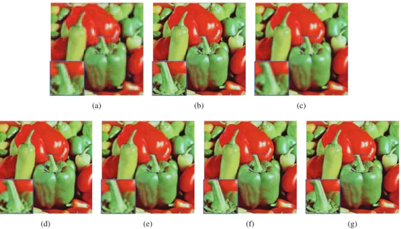
image SR problem with the “pepper” image and standard Tikhonov/Gaussian regularization corresponding to the opti-mization problem formulated in (14). The size of the ground truth HR image shown in Fig. 2(b) is 512×512. Fig. 2(c)–2(f) show the restored images with bicubic interpolation, the pro-posed analytical solution given in Algo. 1 and the splitting algorithm ADMM of [18] adapted to a Gaussian prior. The prior mean image ¯x (approximated HR image) is the up-sampled version of the LR image by bicubic interpolation (Case 1) with the results in Fig. 2(e) and 2(d), whereas ¯x is the ground truth (Case 2) with the results in Fig. 2(g) and 2(f). The regularization parameter was τ = 1 in Case 1 and τ = 0.1 in Case 2. The numerical results corresponding to this experiment are summarized in Table I. The visual impression and the numerical results show that the reconstructed HR images obtained with our method are similar to those obtained with ADMM. However, the proposed FSR method performs much
Fig. 2. SR of the pepper image when considering an ℓ2–ℓ2-model in the image domain: visual results. The prior image mean ¯x is defined as the bicubic
interpolated LR image in Case 1 and as the ground truth HR image in Case 2. (a) Observation.2 (b) Ground truth. (c) Bicubic interpolation. (d) Case 1: ADMM. (e) Case 1: Algo. 1. (f) Case 2: ADMM. (g) Case 2: Algo. 1.
TABLE I
SROF THEPEPPERIMAGEWHENCONSIDERING ANℓ2–ℓ2-MODEL IN THEIMAGEDOMAIN: QUANTITATIVERESULTS
faster than ADMM. More precisely, the computational time with our method is divided by a factor of 60 for Case 1 and by a factor of 80 for Case 2. Note also that the restored images obtained with Case 2 (¯x set to the ground truth) are visually much better than the ones obtained with Case 1 (¯x equal to the interpolated LR image), as expected.
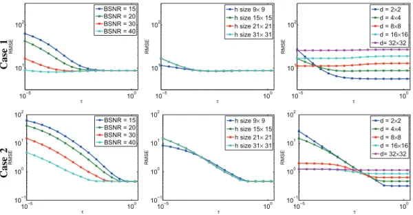
The performance of the proposed method has been also evaluated with various experimental parameters, namely, the BSNR level, the size of the blurring kernel and the decimation factors. The corresponding RMSEs are depicted in Fig. 3 as functions of the regularization parameter τ for the two considered scenarios (Cases 1 and 2). Note that the same performance is obtained by the ADMM-based SR technique since it solves the same optimization problem.
b) Motion blurring kernel: This paragraph considers a
dataset composed of images that have been captured by a camera placed on a tripod, whose Z-axis rotation handle has been locked and X- and Y-axis rotation handles have been 2Note that the LR images have been scaled for better visualization in
this figure (i.e., the actual LR images contain d times fewer pixels than the corresponding HR images).
TABLE II
SROF THEMOTIONBLURREDIMAGEWHENCONSIDERING AN
ℓ2–ℓ2-MODEL IN THEIMAGEDOMAIN: QUANTITATIVERESULTS
loosen [50]. The corresponding dataset is available online.3
The observed LR image, motion kernel and corresponding SR results are shown in Fig. 4. The size of the motion kernel is 19 ×19. As in the previous paragraph, the prior mean image ¯x is the bicubic interpolation of the LR image in Case 1, while ¯x is the ground truth in Case 2. The regularization parameter is set to τ = 0.01 and τ = 0.1 in Cases 1 and 2, respectively. Quantitative results are reported in Table II and show that the proposed method provides competitive results w.r.t. the other methods, while being more computational efficient.
2)ℓ2− ℓ2 Model in the Gradient Domain: This section
compares the performance of the proposed fast SR strat-egy with the gradient profile regularization proposed in [8]. As shown in Section III-A, Theorem 1 allows an analytical SR solution to be computed. The “face” image (of size 276 × 276) shown in Fig. 5(b) was used for these tests. In this experiment, ¯∇x is calculated using the reference HR image and the regularization parameters have been set to 3Available online at http://www.wisdom.weizmann.ac.il/∼levina/papers/
Fig. 3. SR of the “pepper” image when considering the ℓ2–ℓ2model in the image domain: RMSE as functions of the regularization parameter τ for various
noise levels (1st column), blurring kernel sizes (2nd column) and decimation factors (3rd column). The results in the 1st column were obtained for dr= dc=4
and 9 × 9 kernel size; in the 2nd column, dr= dc=4 and BSNR= 30 dB; in the 3rd column, the kernel size was 9 × 9 and BSNR= 30 dB.
Fig. 4. SR of the motion blurred image when considering an ℓ2–ℓ2-model in the image domain: visual results. The prior image mean ¯x is defined as
the bicubic interpolated LR image in Case 1 and as the ground truth HR image in Case 2. (a) Observation. (b) Ground truth. (c) Bicubic interpolation. (d) Case 1: ADMM. (e) Case 1: Algo. 1. (f) Case 2: ADMM. (g) Case 2: Algo. 1.
τ =10−3 and σ = 10−8. The proposed method is compared with the ADMM as well as the conjugate gradient (CG) method instead of the gradient descent (GD) method initially proposed in [17] (since CG has shown to be much more efficient than GD in this experiment). The restored images using bicubic interpolation, ADMM, the CG method and the proposed Algo. 2 are shown in Fig. 5(c)-5(e). The correspond-ing numerical results are reported in Table III. These results illustrate the superiority of the approach in terms of compu-tational time. This significant difference can be explained by the non-iterative nature of the proposed method compared to CG and ADMM. Moreover, all the three methods converge to
the same global minimum as shown by the objective curves in Fig. 6. The convergence of the objective curves is in agreement with the visual and numerical results.
3) Learning-Based ℓ2-Norm Regularization: This section
studies the performance of the algorithm obtained when the analytical solution of Theorem 1 is embedded in the learning-based method of [7]. The method investi-gated in [7] computed an initial estimation of the HR image via SC and used a BP procedure to improve the SR performance. The BP operation was performed by a GD method in [7]. Here, this GD step has been replaced by the analytical solution provided by Theorem 1 and Algo. 1.
Fig. 5. SR of the face image when considering an ℓ2–ℓ2-model in the
gradient domain: visual results. (a) Observation. (b) Ground truth. (c) Bicubic. (d) ADMM. (e) CG [8]. (f) Algo. 2.
TABLE III
SROF THEFACEIMAGEWHENCONSIDERING ANℓ2–ℓ2-MODEL IN THEGRADIENTDOMAIN: QUANTITATIVERESULTS
Fig. 6. SR of the face image when considering an ℓ2–ℓ2-model in the
gradient domain: objective functions.
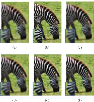
The image “zebra” was used in this experiment to compare the performance of both algorithms.4 The LR and HR images
(of size 300 × 200) are shown in Fig. 7(a) and 7(b). The regularization parameter was set to τ = 0.1. The restored images shown in Figs. 7(c)-7(e) were obtained using the initial SC estimation proposed in [7], the back-projected SC image combined with the GD algorithm of [7] (referred to as “SC + GD”) and the proposed closed-form solution (referred to as “SC + Algo. 1”). The corresponding numerical results are reported in Table IV. The restored images obtained with 4For comparison purpose, the authors used the MATLAB code
correspond-ing to [7] available at http://www.ifp.illinois.edu/∼jyang29.
Fig. 7. SR of the zebra image when considering a learning-based ℓ2-norm
regularization: visual results. (a) Observation. (b) Ground truth. (c) Bicubic. (d) SC [7]. (e) SC+GD [7]. (f) SC+Algo. 1.
TABLE IV
SROF THEZEBRAIMAGEWHENCONSIDERING ALEARNING-BASED
ℓ2-NORMREGULARIZATION: QUANTITATIVERESULTS
the two BP approaches are clearly better than the restoration obtained with the SC method. While the quality of the images obtained with these projection approaches is similar, the use of the analytical solution of Theorem 1 allows the computational cost of the GD step to be reduced significantly.
B. Embedding theℓ2–ℓ2 Analytical Solution Into
the ADMM Framework
In this second group of experiments, we consider two non-Gaussian priors that have been widely used for image reconstruction problems: the TV regularization in the spatial domain and the ℓ1-norm regularization in the wavelet domain.
In both cases, the analytical solution of Theorem 1 is embed-ded into a standard ADMM algorithm inspired from [18] (the resulting algorithms referred to as Algo. 4 and 5 are detailed in Appendix B). The stopping criterion for both implementations is chosen as the relative cost function error defined as
| f (xk+1) − f (xk)|
f(xk) (31)
where f (x) = 12ky − SHxk22 + τ φ(Ax). Note that other stopping criteria such as those studied in [51] could also be
Fig. 8. SR of the Monarch, Lena and Barbara images when considering a TV-regularization: visual results.
investigated. The 512 × 512 images “Lena”, “monarch” and “Barbara” were considered in these experiments. The observed LR images and the HR images (ground truth) are displayed in Fig. 8 (first two columns).
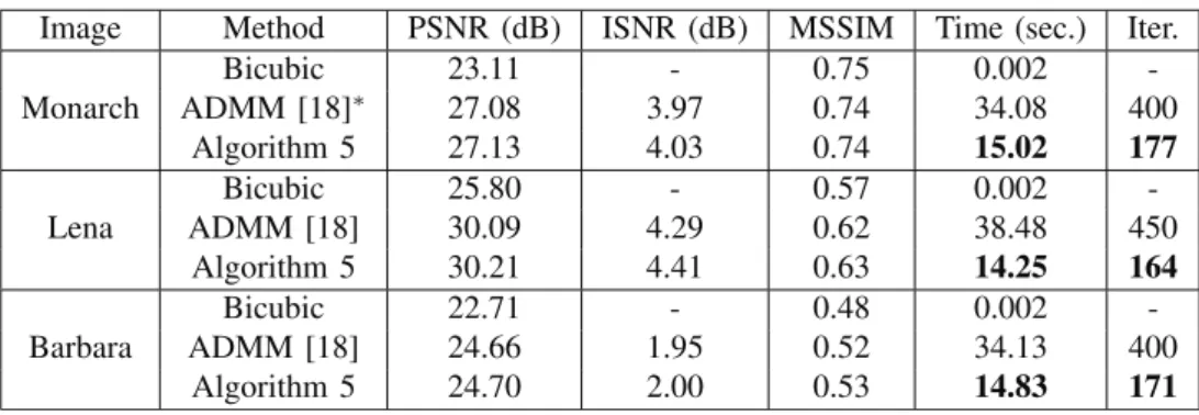
1) TV-Regularization: The regularization parameter was
manually fixed (by cross validation) to τ = 2 × 10⁻³ for the
image “Lena”, to τ = 1.8 × 10⁻³ for the image “monarch”
and to τ = 2.5 × 10⁻³for the image “Barbara”. Fig. 8 shows
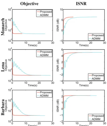
the SR results obtained using the bicubic interpolation (third column), ADMM based algorithm of [18] (fourth column) and the proposed Algo. 4 (last column). As expected, the ADMM reconstructions perform much better than a simple interpolation of the LR image that is not able to solve the upsampling and deblurring problem. The results obtained with the proposed algorithm and with the method of [18] are visually very similar. This visual inspection is confirmed by the quantitative results provided in Table V. However, the proposed algorithm has the advantage of being much faster than the algorithm of [18] (with computational times reduced by a factor larger than 2). Moreover, Fig. 9 illustrates the convergence of the two algorithms. The proposed single image SR algorithm (Algo. 4) converges faster and with less fluctu-ations than the algorithm of [18]. This result can be explained by the fact that the algorithme in [18] requires to handle more variables in the ADMM scheme than the proposed algorithm.
Fig. 9. SR of the Monarch, Lena and Barbara images when considering a TV-regularization: objective function (left) and ISNR (right) vs time.
2)ℓ1-Norm Regularization in the Wavelet Domain: This
section evaluates the performance of Algo. 5, which is com-pared with a generalization of the method proposed in [18]
TABLE V
SROF THEMONARCH, LENA ANDBARBARAIMAGESWHENCONSIDERING ATV-REGULARIZATION: QUANTITATIVERESULTS
Fig. 10. SR of the Monarch, Lena and Barbara images when considering a ℓ1-norm regularization in the wavelet domain: visual results.
to an ℓ1-norm regularization in the wavelet domain. The
motivations for working in the wavelet domain are essentially to take advantage of the sparsity of the wavelet coefficients. All experiments were conducted using the discrete Haar wavelet transform and the Rice wavelet toolbox [52]. For both implementations, the regularization parameter was adjusted by cross validation, leading to τ = 2×10⁻⁴for the image “Lena”,
τ =1.8 × 10⁻⁴for the image “Monarch” and τ = 2.5 × 10⁻⁴ for the image “Barbara”.
Fig. 10 shows the SR reconstruction results with an ℓ1-norm minimization in the wavelet domain. The HR images
Fig. 11. SR of the Monarch, Lena and Barbara images when considering an ℓ1-norm regularization in the wavelet domain: objective function (left) and
PSNR (right) vs time.
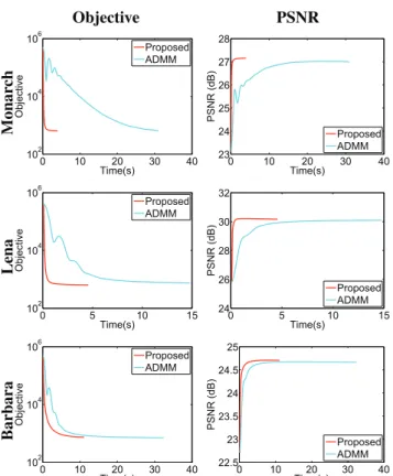
obtained with Algo. 5 and with the algorithm of [18] adapted to the ℓ1-norm prior are visually similar and better than a
simple interpolation. The numerical results shown in Table VI confirm that the two algorithms provide similar reconstruction performance. However, as in the previous case (TV regulariza-tion), the proposed algorithm is characterized by much smaller computational times than the standard ADMM implementa-tion. The faster and smoother convergence obtained with the proposed method (Algo. 5) can be observed in Fig. 11. Note that the fluctuations of the objective function and PSNR values (versus the number of iterations) obtained with the method of [18] are due to the variable splitting, which requires more variables and constraints to be handled than for the proposed method.
TABLE VI
SROF THEMONARCH, LENA ANDBARBARAIMAGESWHENCONSIDERING Aℓ1-NORMREGULARIZATION IN THEWAVELETDOMAIN: QUANTITATIVERESULTS
VI. CONCLUSION ANDPERSPECTIVES
This paper studied a new fast single image super-resolution method based on the widely used image formation model. The proposed resolution approach computed the super-resolved image efficiently by exploiting intrinsic properties of the decimation and the blurring operators in the frequency domain. A large variety of priors was shown to be able to be handled by the proposed super-resolution scheme. Specifically, when considering an ℓ2-regularization, the target image was
computed analytically, getting rid of any iterative steps. For more complex priors (i.e., non ℓ2-regularization), variable splitting allowed this analytical solution to be embedded into the augmented Lagrangian framework, thus accelerating various existing schemes for single image super-resolution. Results on several natural images confirmed the computational efficiency of the proposed approach and showed its fast and smooth convergence. As a perspective of this work, an interest-ing research track consists of extendinterest-ing the proposed method to some online applications such as video super-resolution and medical imaging, to evaluate its robustness to non-Gaussian noise and to extend it to semi-blind or blind deconvolution or multi-frame super-resolution. Considering a more practical case for super-resolving real images compressed by JPEG or JPEG-2000 algorithms would also deserve further exploration.
APPENDIXA
DERIVATION OF THEANALYTICALSOLUTION(13)
The computational details for obtaining the result in (13) from (7) are summarized hereinafter. First, denoting
r = HHSHy +2τ AHv, the solution (7) is
ˆx = (HHSH +2τ AHA)−1r
= FH)3HFSFH3+2τ FAHAFH*−1Fr. (32)
Based on Lemma 1, 3HFSFH3is computed as
3HFSFH3 = 1 d3 H' Jd⊗ INl ( 3 (33) = 1 d3 H))1 d1Td * ⊗'INlINl (* 3 (34) = 1 d3 H'1 d⊗ INl ( ) 1Td ⊗ INl * 3 (35)
Algorithm 4 FSR With TV Regularization
= 1 d 3 H[I Nl, · · · , INl ! "# $ d ]T [INl, · · · , INl ! "# $ d ]3 (36) = 1 d3 H3 . (37)
Note that (34) was obtained from (33) by replacing Jd by
1d1Td, where 1d ∈ Rd×1 is a vector of ones. Obtaining (35)
from (34) is straightforward using the following property of the Kronecker product ⊗
Algorithm 5FSR With ℓ1-Norm Regularization in the Wavelet Domain In (36), 3 ∈ RNh×Nh whereas 5I Nl, · · · , INl 6 ∈ RNl×Nh and 5 INl, · · · , INl 6T
∈ RNh×Nl are block matrices whose blocks
are equal to the identity matrix INl. The matrix 3 ∈ R
Nl×Nh in (37) is given by 3= [IN l, · · · , INl]3 = [INl, · · · , INl]diag{31, · · · , 3d} = [INl, · · · , INl] 31 · · · 0 .. . . .. ... 0 · · · 3d (38) = [31, 32, · · · , 3d]. (39)
As a consequence, (32) can be written as in (9), i.e., ˆx = FH% 1 d3 H3+2τ FAH AFH &−1 Fr (40) = FH = 1 2τ9− 1 2τ93 H % dINl+ 1 2τ393 H &−1 39 1 2τ > Fr (41) = 1 2τF H9Fr − 1 2τF H93H)2τ dI Nl + 393 H*−139Fr (42) where 9 = F'AHA(−1FH. The Lemma 2 is adopted from
(40) to (41) with A1 = 2τ FAHAFH, A2 = 3H, A3 = 1dI
and A4 = 3. Note that the matrices A1 and A3 are always
invertible, implying that the Woodbury formula can be applied. APPENDIXB
PSEUDOCODES OF THEPROPOSEDFASTADMM SUPER-RESOLUTIONMETHODS FORTVAND
ℓ1-NORMREGULARIZATIONS
See Algorithms 4 and 5.
REFERENCES
[1] S. C. Park, M. K. Park, and M. G. Kang, “Super-resolution image reconstruction: A technical overview,” IEEE Signal Process. Mag., vol. 20, no. 3, pp. 21–36, May 2003.
[2] G. Martín and J. M. Bioucas-Dias, “Hyperspectral compressive acquisition in the spatial domain via blind factorization,” in Proc.
IEEE Workshop Hyperspectral Image Signal Process., Evol. Remote Sens. (WHISPERS), Tokyo, Japan, Jun. 2015, pp. 1–4.
[3] J. Yang and T. Huang, “Image super-resolution: Historical overview and future challenges,” in Super-Resolution Imaging. Boca Raton, FL, USA: CRC Press, 2010, pp. 20–34.
[4] T. Akgun, Y. Altunbasak, and R. M. Mersereau, “Super-resolution reconstruction of hyperspectral images,” IEEE Trans. Image Process., vol. 14, no. 11, pp. 1860–1875, Nov. 2005.
[5] I. Yanovsky, B. H. Lambrigtsen, A. B. Tanner, and L. A. Vese, “Efficient deconvolution and super-resolution methods in microwave imagery,”
IEEE J. Sel. Topics Appl. Earth Observ. Remote Sens., vol. 8, no. 9, pp. 4273–4283, Sep. 2015.
[6] R. Morin, A. Basarab, and D. Kouamé, “Alternating direction method of multipliers framework for super-resolution in ultrasound imaging,” in Proc. 9th IEEE Int. Symp. Biomed. Imag. (ISBI), Barcelona, Spain, May 2012, pp. 1595–1598.
[7] J. Yang, J. Wright, T. S. Huang, and Y. Ma, “Image super-resolution via sparse representation,” IEEE Trans. Image Process., vol. 19, no. 11, pp. 2861–2873, Nov. 2010.
[8] J. Sun, J. Sun, Z. Xu, and H.-Y. Shum, “Image super-resolution using gradient profile prior,” in Proc. IEEE Conf. Comput. Vis. Pattern
Recognit. (CVPR), Anchorage, AK, USA, Jun. 2008, pp. 1–8. [9] Y.-W. Tai, S. Liu, M. S. Brown, and S. Lin, “Super resolution using edge
prior and single image detail synthesis,” in Proc. IEEE Conf. Comput.
Vis. Pattern Recognit. (CVPR), San Francisco, CA, USA, Jun. 2010,
pp. 2400–2407.
[10] P. Thévenaz, T. Blu, and M. Unser, “Image interpolation and resam-pling,” in Handbook of Medical Imaging, I. N. Bankman, Ed. Orlando, FL, USA: Academic, 2000, pp. 393–420.
[11] X. Zhang and X. Wu, “Image interpolation by adaptive 2-D autore-gressive modeling and soft-decision estimation,” IEEE Trans. Image
Process., vol. 17, no. 6, pp. 887–896, Jun. 2008.
[12] S. Mallat and Y. Guoshen, “Super-resolution with sparse mixing esti-mators,” IEEE Trans. Image Process., vol. 19, no. 11, pp. 2889–2900, Nov. 2010.
[13] W. T. Freeman, E. C. Pasztor, and O. T. Carmichael, “Learning low-level vision,” Int. J. Comput. Vis., vol. 40, no. 1, pp. 25–47, Oct. 2000. [14] D. Glasner, S. Bagon, and M. Irani, “Super-resolution from a single
image,” in Proc. IEEE Int. Conf. Comput. Vis. (ICCV), Kyoto, Japan, Sep./Oct. 2009, pp. 349–356.
[15] J.-B. Huang, A. Singh, and N. Ahuja, “Single image super-resolution from transformed self-exemplars,” in Proc. IEEE Conf. Comput.
Vis. Pattern Recognit. (CVPR), Boston, MA, USA, Jun. 2015,
pp. 5197–5206.
[16] R. Zeyde, M. Elad, and M. Protter, “On single image scale-up using sparse-representations,” in Curves and Surfaces (Lecture Notes in Com-puter Science), J.-D. Boissonnat et al., Eds. Heidelberg, Germany: Springer, 2012, pp. 711–730.
[17] J. Sun, J. Sun, Z. Xu, and H.-Y. Shum, “Gradient profile prior and its applications in image super-resolution and enhancement,” IEEE Trans.
Image Process., vol. 20, no. 6, pp. 1529–1542, Jun. 2011.
[18] M. K. Ng, P. Weiss, and X. Yuan, “Solving constrained total-variation image restoration and reconstruction problems via alternating direction methods,” SIAM J. Sci. Comput., vol. 32, no. 5, pp. 2710–2736, 2010.
[19] A. Beck and M. Teboulle, “A fast iterative shrinkage-thresholding algorithm for linear inverse problems,” SIAM J. Imag. Sci., vol. 2, no. 1, pp. 183–202, Mar. 2009.
[20] A. Marquina and S. J. Osher, “Image super-resolution by TV-regularization and Bregman iteration,” J. Sci. Comput., vol. 37, no. 3, pp. 367–382, Dec. 2008.
[21] W. Yin, S. Osher, D. Goldfarb, and J. Darbon, “Bregman iterative algo-rithms for ℓ1-minimization with applications to compressed sensing,”
SIAM J. Imag. Sci., vol. 1, no. 1, pp. 143–168, 2008.
[22] M. D. Robinson, C. A. Toth, J. Y. Lo, and S. Farsiu, “Efficient Fourier-wavelet super-resolution,” IEEE Trans. Image Process., vol. 19, no. 10, pp. 2669–2681, Oct. 2010.
[23] F. Šroubek, J. Kamenický, and P. Milanfar, “Superfast superresolution,” in Proc. IEEE Int. Conf. Image Process. (ICIP), Brussels, Belgium, Sep. 2011, pp. 1153–1156.
[24] M. Ebrahimi and E. R. Vrscay, “Regularization schemes involving self-similarity in imaging inverse problems,” in Proc. 4th AIP Int. Conf., 1st
Congr. IPIA, 2008, pp. 1–12.
[25] K. Zhang, X. Gao, D. Tao, and X. Li, “Single image super-resolution with non-local means and steering kernel regression,” IEEE Trans. Image
Process., vol. 21, no. 11, pp. 4544–4556, Nov. 2012.
[26] M. Elad and A. Feuer, “Restoration of a single superresolution image from several blurred, noisy, and undersampled measured images,” IEEE
Trans. Image Process., vol. 6, no. 12, pp. 1646–1658, Dec. 1997.
[27] S. Farsiu, D. Robinson, M. Elad, and P. Milanfar, “Advances and challenges in super-resolution,” Int. J. Imag. Syst. Technol., vol. 14, no. 2, pp. 47–57, 2004.
[28] Z. Lin and H.-Y. Shum, “Fundamental limits of reconstruction-based superresolution algorithms under local translation,” IEEE Trans. Pattern
Anal. Mach. Intell., vol. 26, no. 1, pp. 83–97, Jan. 2004.
[29] J. K. H. Ng, “Restoration of medical pulse-echo ultrasound images,” Ph.D. dissertation, Dept. Eng., Trinity College, Univ. Cambridge, Cambridge, U.K., 2006.
[30] N. Zhao, A. Basarab, and D. Kouamé, and J.-Y. Tourneret. (2015). “Joint segmentation and deconvolution of ultrasound images using a hierarchical Bayesian model based on generalized Gaussian priors.” [Online]. Available: http://arxiv.org/abs/1412.2813
[31] C. P. Robert, The Bayesian Choice: From Decision-Theoretic
Founda-tions to Computational Implementation (Springer Texts in Statistics), 2nd ed. New York, NY, USA: Springer-Verlag, 2007.
[32] A. Gelman, J. B. Carlin, H. S. Stern, D. B. Dunson, A. Vehtari, and D. B. Rubin, Bayesian Data Analysis, 3rd ed. Boca Raton, FL, USA: CRC Press, 2013.
[33] N. Nguyen, P. Milanfar, and G. Golub, “A computationally efficient superresolution image reconstruction algorithm,” IEEE Trans. Image
Process., vol. 10, no. 4, pp. 573–583, Apr. 2001.
[34] Q. Wei, J. Bioucas-Dias, N. Dobigeon, and J.-Y. Tourneret, “Hyperspec-tral and multispec“Hyperspec-tral image fusion based on a sparse representation,”
IEEE Trans. Geosci. Remote Sens., vol. 53, no. 7, pp. 3658–3668,
Jul. 2015.
[35] H. A. Aly and E. Dubois, “Image up-sampling using total-variation regularization with a new observation model,” IEEE Trans. Image
Process., vol. 14, no. 10, pp. 1647–1659, Oct. 2005.
[36] J. M. Bioucas-Dias, “Bayesian wavelet-based image deconvolution: A GEM algorithm exploiting a class of heavy-tailed priors,” IEEE Trans.
Image Process., vol. 15, no. 4, pp. 937–951, Apr. 2006.
[37] J. Ng, R. Prager, N. Kingsbury, G. Treece, and A. Gee, “Wavelet restoration of medical pulse-echo ultrasound images in an EM frame-work,” IEEE Trans. Ultrason., Ferroelectr., Freq. Control, vol. 54, no. 3, pp. 550–568, Mar. 2007.
[38] C. V. Jiji, M. V. Joshi, and S. Chaudhuri, “Single-frame image super-resolution using learned wavelet coefficients,” Int. J. Imag. Syst.
Technol., vol. 14, no. 3, pp. 105–112, 2004.
[39] M. A. T. Figueiredo and R. D. Nowak, “An EM algorithm for wavelet-based image restoration,” IEEE Trans. Image Process., vol. 12, no. 8, pp. 906–916, Aug. 2003.
[40] R. Fattal, “Edge-avoiding wavelets and their applications,” ACM Trans.
Graph., vol. 28, no. 3, pp. 1–10, Aug. 2009.
[41] S. Roth and M. J. Black, “Fields of experts: A framework for learning image priors,” in Proc. IEEE Conf. Comput. Vis. Pattern
Recognit. (CVPR), Jun. 2005, pp. 860–867.
[42] D. Zoran and Y. Weiss, “From learning models of natural image patches to whole image restoration,” in Proc. IEEE Int. Conf. Comp. Vis. (ICCV), Barcelona, Spain, Nov. 2011, pp. 479–486.
[43] H. W. Engl, M. Hanke, and A. Neubauer, Regularization inverse
problems. Springer Science & Business Media, 1996, vol. 375.
[44] O. Féron, F. Orieux, and J.-F. Giovannelli. (2015). “Gradient scan Gibbs sampler: An efficient algorithm for high-dimensional Gaussian distributions.” [Online]. Available: http://arxiv.org/abs/1509.03495 [45] F. Orieux, O. Féron, and J. F. Giovannelli, “Sampling high-dimensional
Gaussian distributions for general linear inverse problems,” IEEE Signal
Process. Lett., vol. 19, no. 5, pp. 251–254, May 2012.
[46] C. Gilavert, S. Moussaoui, and J. Idier, “Efficient Gaussian sampling for solving large-scale inverse problems using MCMC,” IEEE Trans. Signal
Process., vol. 63, no. 1, pp. 70–80, Jan. 2015.
[47] W. W. Hager, “Updating the inverse of a matrix,” SIAM Rev., vol. 31, no. 2, pp. 221–239, 1989.
[48] Q. Wei, N. Dobigeon, and J.-Y. Tourneret, “Bayesian fusion of multi-band images,” IEEE J. Sel. Topics Signal Process., vol. 9, no. 6, p. 1127, Sep. 2015.
[49] Z. Wang, A. C. Bovik, H. R. Sheikh, and E. P. Simoncelli, “Image quality assessment: From error visibility to structural similarity,” IEEE
Trans. Image Process., vol. 13, no. 4, pp. 600–612, Apr. 2004.
[50] A. Levin, Y. Weiss, F. Durand, and W. T. Freeman, “Understanding and evaluating blind deconvolution algorithms,” in Proc. IEEE Conf.
Comput. Vis. Patt. Recognit. (CVPR), Miami, FL, USA, Jun. 2009, pp. 1964–1971.
[51] S. Boyd, N. Parikh, E. Chu, B. Peleato, and J. Eckstein, “Distributed optimization and statistical learning via the alternating direction method of multipliers,” Found. Trends Mach. Learn., vol. 3, no. 1, pp. 1–122, Jan. 2011.
[52] R. Baraniuk et al. Rice Wavelet Toolbox, accessed on Dec. 1, 2002. [Online]. Available: http://dsp.rice.edu/software/rice-wavelet-toolbox
Ningning Zhao received the B.Sc. degree from Jilin University, China, in 2011, the master’s degree from the Electrical Engineering Department, Beihang University, Beijing, China, in 2012, and the M.Sc. degree from the University of Toulouse, France, in 2013, where she is currently pursuing the Ph.D. degree. She is currently with the Signal and Communication Group and also Image Comprehen-sion and Processing Group with IRIT Laboratory. Her research interests include medical imaging and inverse problems of image processing, particularly image deconvolution and segmentation. He has served as a Reviewer of the IEEE TRANSACTIONS ONIMAGEPROCESS.
Qi Wei(S’13) was born in Shanxi, China, in 1989. He received the Ph.D. degree in signal and image processing from the National Polytechnic Institute of Toulouse, University of Toulouse, France, in 2015, and the bachelor’s degree in electrical engineering from Beihang University, Beijing, China, in 2010. His Ph.D. thesis, Bayesian Fusion of Multi-band Images: A Powerful Tool for Super-Resolution, was rated as one of the best theses (received Prix Lèopold Escande) with University of Toulouse, in 2015. In 2012, he was an Visiting Student with the Signal Processing and Communications Group, Department of Signal Theory and Communications, Universitat Politècnica de Catalunya. Since 2015, he has been a Research Associate with the Signal Processing Laboratory, Department of Engineering, University of Cambridge. His research has been focused on inverse problems in image processing, Bayesian statistical inference and parameter estimation, and optimization algorithms in large scale data processing. He has served as a Reviewer of the IEEE TRANSACTION ON
IMAGEPROCESS, the IEEE JOURNAL OFSELECTEDTOPICS INSIGNAL
PROCESSING, the IEEE TRANSACTIONS ONGEOSCIENCE ANDREMOTE
SENSING, and several conferences.
Adrian Basarab received the M.S. and Ph.D. degrees in signal and image processing from the National Institute for Applied Sciences of Lyon, France, in 2005 and 2008, respectively. Since 2009, he has been an Assistant Professor with the Univer-sity Paul Sabatier Toulouse 3 and a member of IRIT laboratory. His research interests include medical imaging, and more particularly motion estimation, inverse problems, and ultrasound image formation. He is an Associate Editor of the Digital Signal
Nicolas Dobigeon (S’05–M’08–SM’13) was born
in Angoulême, France, in 1981. He received the Engineering degree in electrical engineering from ENSEEIHT, Toulouse, France, in 2004, and the M.Sc. degree in signal processing from INP Toulouse, in 2004, the Ph.D. degree and the Habili-tation à Diriger des Recherches in signal processing from INP Toulouse, in 2007 and 2012, respectively. From 2007 to 2008, he was a Post-Doctoral Research Associate with the Department of Electrical Engineering and Computer Science, University of Michigan, Ann Arbor. Since 2008, he has been with INP-ENSEEIHT Toulouse, University of Toulouse, where he is currently an Associate Profes-sor. He conducts his research within the Signal and Communications Group, IRIT Laboratory, and he is also an Affiliated Faculty Member of the TeSA Laboratory. His recent research activities have been focused on statistical signal and image processing, with a particular interest in Bayesian inverse problems with applications to remote sensing and biomedical imaging.
Denis Kouamé (M’97) received the Ph.D. and Habilitation à Diriger des Recherches degrees in sig-nal processing and medical ultrasound imaging from the University of Tours, Tours, France, in 1996 and 2004, respectively. He is currently a Professor with the Paul Sabatier University of Toulouse, Toulouse, France, and a member of the IRIT Laboratory. From 1998 to 2008, he was an Assistant and then an Associate Professor with the University of Tours. From 1996 to 1998, he was a Senior Engineer with the GIP Tours, Tours, France. He was the Head of the Signal and Image Processing Group, and then the Head of Ultrasound Imaging Group, Ultrasound and Signal Laboratory, University of Tours, from 2000 to 2006 and from 2006 to 2008. He currently leads the Image Comprehension and Processing Group, IRIT. His research interests are focused on signal and image processing with applications to medical imaging and particularly ultrasound imaging, including high resolution imaging, image resolution enhancement, doppler signal processing, detection and estimation with application to cerebral emboli detection, multidimensional parametric modeling, spectral analysis, and inverse problems related to compressed sensing and restoration. He has been involved in the organization of several conferences. He has also led a number of invited conferences, special sessions and tutorials in this area at several IEEE conferences and workshops. He has been serving as an Associate Editor of the IEEE TRANSACTIONS ON
ULTRASONICS, FERROELECTRICS,ANDFREQUENCYCONTROL.
Jean-Yves Tourneret (SM’08) received the
Ingénieur degree in electrical engineering from the University of Toulouse, Toulouse, in 1989, and the Ph.D. degree from the INP Toulouse, in 1992. He is currently a Professor with the University of Toulouse and a member of the IRIT Laboratory. His research activities are centered around statistical signal and image processing with a particular interest to Bayesian and Markov chain Monte Carlo methods. He has been involved in the organization of several conferences, including the European Conference on Signal Processing in 2002 (Program Chair), the international conference ICASSP’6 (plenaries), the Statistical Signal Processing Workshop 2012 (International Liaisons), the International Workshop on Computational Advances in Multi-Sensor Adaptive Processing in 2013 (local arrangements), the Statistical Signal Processing Workshop in 2014 (special sessions), the Workshop on Machine Learning for Signal Processing in 2014 (special sessions). He has been the General Chair of the CIMI Workshop on Optimization and Statistics in Image processing hold in Toulouse, in 2013 (with F. Malgouyres and D. Kouamé) and of the International Workshop on Computational Advances in Multi-Sensor Adaptive Processing in 2015 (with P. Djuric). He has been a member of different technical committees including the Signal Processing Theory and Methods Committee of the IEEE Signal Processing Society (2001–2007, 2010–2015). He has been serving as an Associate Editor of the IEEE TRANSACTIONS ONSIGNAL
PROCESSING(2008–2011, 2015-present) and for the EURASIP journal on