Literature Review on the Modeling of Fire Growth and Smoke Movement

(1)

Publisher’s version / Version de l'éditeur:

Vous avez des questions? Nous pouvons vous aider. Pour communiquer directement avec un auteur, consultez la première page de la revue dans laquelle son article a été publié afin de trouver ses coordonnées. Si vous n’arrivez pas à les repérer, communiquez avec nous à PublicationsArchive-ArchivesPublications@nrc-cnrc.gc.ca.

Questions? Contact the NRC Publications Archive team at

PublicationsArchive-ArchivesPublications@nrc-cnrc.gc.ca. If you wish to email the authors directly, please see the first page of the publication for their contact information.

https://publications-cnrc.canada.ca/fra/droits

L’accès à ce site Web et l’utilisation de son contenu sont assujettis aux conditions présentées dans le site LISEZ CES CONDITIONS ATTENTIVEMENT AVANT D’UTILISER CE SITE WEB.

Research Report (National Research Council of Canada. Institute for Research in

Construction), 2003-08-28

READ THESE TERMS AND CONDITIONS CAREFULLY BEFORE USING THIS WEBSITE. https://nrc-publications.canada.ca/eng/copyright

NRC Publications Archive Record / Notice des Archives des publications du CNRC :

https://nrc-publications.canada.ca/eng/view/object/?id=c2db079c-5bee-4419-a4f6-9c5da7c0b2c5 https://publications-cnrc.canada.ca/fra/voir/objet/?id=c2db079c-5bee-4419-a4f6-9c5da7c0b2c5

Archives des publications du CNRC

For the publisher’s version, please access the DOI link below./ Pour consulter la version de l’éditeur, utilisez le lien DOI ci-dessous.

https://doi.org/10.4224/20378835

Access and use of this website and the material on it are subject to the Terms and Conditions set forth at

Literature Review on the Modeling of Fire Growth and Smoke

Movement

(2)

Literature Review on the Modeling of Fire Growth and Smoke

Movement

Bounagui, A.; Bénichou, N.

IRC-RR-139

August 28, 2003

(3)

ABSTRACT

Countries worldwide are moving toward performance-based codes which will establish a level of safety that specifies the performance of the building and its components. Fire growth and smoke movement models are a tool in the evaluation of the performance buildings with its materials and contents. In recent years, development of fire growth and smoke movement models has increased and a selection of these models is reviewed in this report. The review has revealed that one of the main inputs to fire growth and smoke movement models is the heat release rate which defines the fire size and its growth. The report also presents the various categories and methods that have been used to evaluate the heat release for each fire growth and smoke movement model. Finally, recommendations on future research are identified.

(4)

2.1.1 Description... 2 2.1.2 Fire Specification... 2 2.2 Ozone... 4 2.2.1 Description... 4 2.2.2 Fire Specification... 4 2.3 Conclusions... 6 3 TWO-ZONE MODELS...6 3.1 Single Compartment... 7 3.1.1 FIRST... 7 3.1.2 ASET... 8 3.2 Multi-Compartment... 9 3.2.1 CFAST/FAST/CCFM.VENTS... 9 3.2.2 FIRM... 10

3.2.3 NRC-Smoke Movement Model... 13

3.2.4 BRANZFIRE... 14 3.2.5 ARGO... 16 3.3 Conclusions... 18 4 FIELD MODELS...18 4.1 FDS... 18 4.1.1 Description... 18 4.1.2 Fire Specification... 19 ii

(5)

4.2 CFX... 19 4.2.1 Description... 19 4.2.2 Fire specification... 20 4.3 JASMINE ... 20 4.3.1 Description... 20 4.3.2 Fire specification... 21 4.4 Conclusions... 21 5 DISCUSSIONS...22 6 CONCLUSIONS...22 7 RECOMMENDATIONS...22 REFERENCES...23 iii

(6)

LIST OF TABLES

Table 1. Conservative Zone Modeling Differential Equations... 6

Table 2. Categories of t-squared fires and appropriate

α

values... 14

Table 3. Heat Release Rate Specification Options... 21

(7)

NOMENCLATURE

v

A Burning surface area

( )

m2

0

A initial pyrolysising area in ceiling

( )

m2

max

A specified maximum pool area

( )

m2

p

c

specific heat at constant pressure

(

J /kg.K

)

v

c

specific heat at constant volume

(

J /kg.K

)

D

pool Diameter

( )

m

t

time

(

s

)

p

t

dummy variable of integration 2

t doubling time for vertical flame spread

( )

s

burnt

t

local burn out time

( )

s

height

t

local burn out time per height of fire object in [s/m]

b

t

burn time

(

s

)

g

T

average gas temperature

( )

K

wi

T

wall temperature inside compartment

( )

K

s

T

surface temperature of burning object

( )

K 0

T

initial temperature of the wall

( )

K

R

mass burning rate

(

kg/min

)

r

∆

enhancement of mass burning rate

(

kg/min

)

eff f

H

_, effective combustion heat of fuel

(

J /kg

)

f

m

. pyrolysis rate

(

kg /s

)

in ox

m

_, mass of oxygen coming in the compartment through vents

( )

kg

i

m

total mass in layer I

( )

kg •

i

m rate of addition of mass into layer I

(

kg/s

)

b

m

.

burning rate

(

kg/s

)

.

m

′′

mass loss rate unit area (

kg

/

m

2.

s

)

. ∞′′

m

mass loss rate per unit area for an infinite pool (

kg

/

m

2.

s

)

P

Pressure

( )

Pa

eff f

H

_, effective combustion heat of fuel

(

J/kg

)

ν

H

∆ heat of vaporization

(

J /kg

)

c

H

∆ heat of combustion

(

J/kg

)

v

(8)

U

h

• rate of additional of enthalpy into upper layer

( )

W

L

h

• rate of additional of enthalpy lower layer

( )

W

c

H

heat of combustion of the fuel

(

J/kg

)

fo

h

initial flame height in

( )

m

object

H

height of the fire object

( )

m

i

E

internal energy in layer I

( )

W

f

Q

.

total heat release rate of the fire

( )

W

.

f

q′′ net heat flux from the burner flame

kW

/ m

2

volume

q

rate of heat release per volume in the flame zone (

kW

/ m

3) .

w

q′′ net heat flux from the burner flame

kW

_{/ m}

2

area

q

rate of heat release per area in the flame zone (

kW

/ m

2)

k extinction-absorption coefficient of the flame (1/m) K flame area constant

(

m /

2

kW

)

1

V net volume of liquid [

m

3] V compartment volume

( )

m

3

f

V

flame spread rate

(

m/min

)

a

V

velocity of the pyrolisis front

(

m

2

/

s

)

Greek Symbols

ε

Emissivity of surface

σ

Stephen Boltstman constant

(

J

/

m

2

.

K

4

.

min

)

ρ

Density of gas, wall or fuel material

(

kg

/ m

3

)

α

constant for a particular fuel of fuel package

(

kW

/ s

2

)

γ

ratio of

v p

c

β

velocity of horizontal flame spread

(

m /s

)

w

τ

time to ignition of the wall lining

(

s

)

c

τ

time to ignition of the ceiling lining

( )

s

(9)

Subscripts

f

fuel

max maximum value

ox oxygen

u upper layer

l lower layer

haz onset of hazardous conditions det detection w wall

i

inside

g

gas 2 O oxygen 2 CO carbon dioxide CO carbon monoxide

soot

soot Abbreviations

RHR

Heat release rate

(10)

Literature Review on the Modeling of Fire Growth and Smoke movement By

A. Bounagui, N. Benichou

1

Introduction

Design for Fire Safety Engineering is increasingly moving towards the use of the performance-based codes due to the restrictive nature of prescriptive codes. Performance evaluation can then use trade-offs between many design options to provide the required level of safety. Fire models are means in the evaluation of the performance of buildings built with new materials and contents. With the need for design tools to aid in demonstrating compliance with performance-based codes, the use of fire modeling techniques has become widely used by designers and practitioners in many area of fire protection design 1.

Fire modeling of a compartment can be achieved either using empirical equations based on observations from experiment or mathematical methods that are commonly divided into two groups: stochastic (probabilistic) and deterministic models 1. The emphasis in this document is on the deterministic models, which predict fire development based on solutions to mathematical equations that describe the physical and chemical behaviour of a fire. There are two types of deterministic compartment fire models: zone models and field models.

The basic assumption used to formulate a zone fire model is that a compartment can be divided into a number of zones, and for each zone, the physical parameters such as gas

temperature and species concentrations are assumed to be uniform. These zones interact by exchanging mass and energy 2. Zone models may be grouped into two types based on the number of control volumes (zones) in each compartment: one-zone models and two-zone models. One-zone models are widely used in the analysis of post-flashover fires. Two-zone models are widely used in the analysis of pre-flashover fires.

Field models are based on an approach that divides an enclosure into a large number of elemental volumes. The model solves the fundamental equations governing the transfer of mass, momentum, and energy between these small volumes to predict the progress of a fire within the enclosure.

A detailed survey of existing fire models can be found in references 3, 4. In this review, we will focus on a representative selection of fire growth and smoke movement models and

investigate how the fire growth is simulated within these models. We will investigate the

parameters that most influence the fire growth, such as the heat release (see reference 5). The review in this report classifies the models into three categories: one-zone models, two-zones models and field models.

2

_{One-zone Models}

One-zone models are widely used in the analysis of post-flashover fires, as well as studying the impact of smoke movement in compartments remote from the fire room. The one-zone modeling concept dates back to the work of Kawagoe, who developed a single-one-zone approach for analyzing a post-flashover fire 6. This approach was the basis of the development of a series of single-zone post-flashover fire models 7.

Over the past two decades, a number of researchers have developed models for the post-flashover fire that predict the smoke movement, smoke concentration in the building and the impact of the temperature on the structure of the building3, 4, 8.

(11)

The selection of the models reviewed in this document is based on the availability of pertinent documentation and references to the validation of these models against experimental data. The models presented here include NRC – Fire growth model and Ozone, with the emphasis on how fire growth is implemented within them.

2.1 NRC – Fire growth model 2.1.1 Description

NRC fire growth model was developed at the National Research Council of Canada and is a component of the fire risk-cost assessment model FiRECAM TM_{which is being developed}

for the evaluation of risk to life and property loss in apartment and office buildings 9. NRC fire growth model can be used to predict the fire growth characteristics for three design fires: flashover fires, non-flashover flaming fires and smouldering fires. This fire growth model

includes a new treatment of the burning rate under vitiated oxygen conditions; includes a better representation of the burning characteristics and combustion efficiency that is dependent on the size of the compartment, and assumes that a fire compartment can be treated as a single reactor.

NRC fire growth model inputs are the compartment size, property data for the wall materials and furniture material, fuel load, and the conditions of the door (open or closed). The outputs are the burning rate, room temperature, wall temperature, air supply rate, oxygen concentration and the production of smoke and toxic gases.

NRC fire growth model was compared with the “FIRST” and “FAST” models, developed at the National Institute of Standards and Technology as well as test data. Results of this comparison can be found in references 9, 10. For the open door case, the predictions were comparable, except for CO concentration where the NRC fire growth model predicts higher values. The higher values, however, are in better agreement with experimental observations. For the closed door case, the NRC fire growth model predicts high values for both CO and CO2 concentrations, whereas the others models predict a basically hazard-free environment. NRC fire growth model is in better agreement with the experimental observations, which show that a fire in a closed-door compartment can still be hazardous.

2.1.2 Fire Specification

In the case of the NRC fire growth model, it models the energy release rate for two types of fire: fuel controlled fire and ventilation-controlled fire using the following expressions:

γµ

R

H

Q

_c =∆ _c (Fuel-controlled fire)

µ

a c c

H

m

Q

=∆ (Ventilation-controlled fire) where:

R

: mass burning rate

(

kg/min

)

a

m

: air ventilation rate

(

kg/min

)

γ

: stiochiometric air to fuel mass ratio

µ

: combustion efficiency

c

H

∆ : heat of combustion

(

J /kg

)

(12)

The model uses the following empirical equations11, 12 to compute the air ventilation rate through the compartment opening:

F

H

n

T

H

A

C

g

m

g o g o D a 5 . 1 5 . 0

1

2

3

2

    ₋                         − =

ρ

(

)

(

)

L

H

B

T

B

F

g

2

100

273

1

+ + − − = where:

g

: gravitational constant

(

m

/

min

2

)

D

C : orifice coefficient

ρ

: average gas density

(

kg

/ m

3

)

A

: door opening area

( )

m

2

H

: door opening height

( )

m

o

T

: ambient temperature

( )

K

g

T

: average gas temperature

( )

K n : height of the neutral plane

( )

m

F

: correction factor

B

: compartment size factor

L

: characteristic compartment length

( )

m

The model uses the empirical relation that was developed by Quintiere 13 to determine the burning rate for smouldering fires:

2

0185

.

0

1 .

0 t

t

R

= + where:

t

: time

( )

min

For flaming fires, the model uses the expression given by Tewarson and Pion 14 to determine the mass burning rate of flexible polyurethane foam:

v v

A

r

NO

H

R

_











∆

+













∆

=

2

ξ

where:

ξ

: constant and is equal to 11.3

(

MJ

/

m

2

.

min

)

for polyurethane foam ν

H

∆

: heat of vaporization

(

J /kg

)

r

∆

: enhancement of the mass burning rate

(

kg/min

)

2

NO : oxygen mole fraction

(13)

v

A

: burning surface area

( )

m

2

2.2 Ozone 2.2.1 Description

Ozone was developed at the Department of Mechanical Material and Structure at Liege University. Again, it is a one-zone model used to predict the temperature in a compartment and to evaluate the structural fire resistance of elements 15.

The Ozone model requires, as inputs the geometry of the compartment, the thermal properties of the materials, the heat release rate, the pyrolysis rate and the fire area as a function of time. Outputs of the model are the gas temperature, wall construction temperatures, and the fire energy release rate. Ozone predictions were compared with full-scale fire tests that have been performed at Cardington, UK, by the British Steel Technical in collaboration with BRE16. Results of this comparison can be found in reference15. The comparison with the large series test shows that the Ozone prediction is very good for a ventilation factor up to 9.3 2

5

m . However for a higher ventilation factor, Ozone is not able to give a good prediction of the fire source.

The model defines the fire source by three parameters, the pyrolysis rate, the heat release rate and the fire area. The estimation of the heat release can be obtained from one of the three combustion models within Ozone. These combustion models have been designed to each represent a different situation where Ozone can be used. The following expressions define the heat release rate used in these combustion models:

a- No combustion model

In this model, the pyrolysis rate and the heat release rate set in the data are used in the mass and energy balances without any modification regarding the oxygen concentration in the compartment. No control by the ventilation is made. For each time step, the following equations are used:

( )

t

m

( )

t

m

f f,data . .

=

( )

t

RHR

( )

t

RHR

=

_data where: f

m

. : pyrolysis rate

(

kg /s

)

data f

m

, .

: pyrolysis rate from the provided data file

(

kg /s

)

RHR

: heat release rate

( )

W

data

RHR

: heat release rate from the provided data file

( )

W

(14)

b- External flaming combustion model

In this model, the pyrolysis rate remains unchanged and if the fire is fuel-controlled and all the mass loss of fuel delivers energy inside the compartment, the model uses the following expressions to calculate the heat release rate:

( )

t

m

( )

t

m

f f,data . .

=

( )

t RHRdata

( )

t mf

( )

t Hf eff RHR _, . = = where: eff f

H

_, : effective combustion heat of fuel

(

J /kg

)

If the fire is ventilation-controlled and the combustion is not complete, the energy released is governed by the mass of oxygen coming into the compartment through vents:

( )

t

m

( )

t

m

f f,data . .

=

( )

feff in ox H t m t RHR , _, . 27 . 1 = where: in ox

m

_, : mass of oxygen coming in the compartment through vents

( )

kg

c- Extended fire duration combustion model

In this model, the release of mass may be limited by the quantity of oxygen available in the compartment. If the fire is fuel-controlled and all the mass loss of fuel delivers energy into the compartment the heat release rate is:

( )

t

m

( )

t

m

f f,data . .

=

( )

t RHRdata

( )

t mf

( )

t Hf eff RHR _, . = =

If the fire is ventilation-controlled, the mass lost by the fire is governed by the mass of oxygen coming into the compartment and the pyrolysis mass is transformed into energy:

( )

27 .

1

. ,

t

m

t

m

_f

=

oxin

( )

feff in ox eff f f H t m H t m t RHR , _, . , . 27 . 1 = =

In this model, no external combustion is assumed. The fire load delivers its energy into the compartment. If the fire is ventilation-controlled, the pyrolysis rate is proportional to the oxygen coming into the compartment.

(15)

2.3 Conclusions

In this section two one-zone models were presented, namely NRC-Fire growth model and Ozone. NRC- Fire growth requires the fire load as input and uses the fire growth sub-model to estimate the heat release rate. Ozone requires heat release as input and uses different combustion model to estimate the heat release rate for a specific scenario. Both models are simple fire growth and smoke movement models. Some of their application is limited to a single compartment with a simple shape; a single fire source; and the physical parameters are

assumed uniform over one zone. However, both models have a practical execution time and run on a personal computer.

3

Two-Zone Models

Zone models are used to calculate the evolving distribution of smoke, fire gases and heat throughout a constructed facility during a fire. In two-zone models, each compartment is divided into two layers. Based on the principle of the conservation of mass and energy, as well as the ideal gas law, a set of ordinary differential equations (ODE) is derived. These

conservation laws are invoked for each zone and are summarized in Table 1. Details of the calculations can be found in reference17. In this type of model, the physical details of the gas within a zone are not considered, however mass and energy transport between zones have to be calculated by modeling the relevant fire sub-processes: combustion and chemistry, fluid flow and heat transfer 18. Quintiere has reviewed the various processes which are associated with fire growth in compartments 19.

Table 1. Conservative Zone Modeling Differential Equations Variables Differential Equations for i’th layer

Mass •

=

_i i

_m

dt

dm

Pressure

)

(

1

L U

h

V

dt

dP

• •

+

−

=

γ

Volume













₋

=

•

dt

dP

V

h

P

dt

dV

i i i

1 ₍

γ

₁

₎

γ

Density       − + − − = • • dt dP V T m C h V T C dt d i i i P i i i P i 1 ) ( 1 γ ρ Temperature       ₋ ₊ = • • dt dP V T m C h V C dt dT i i i P i i i P i 1 ₍ ₎

ρ

Internal Energy













₊

=

•

dt

dP

V

h

dt

dE

i i i

γ

1

Equations in Table 1 predict, as functions of time, quantities such as pressure, layer heights and temperatures given the accumulation of mass and enthalpy in the two layers.

Two-zone models are used to model and analyze pre-flashover fires. Quintiere has mentioned that the two-zone fire modeling of pre-flashover fires emerged in the mid-1970s with

(16)

the publication of a basis for the zone model approach by Fowkes in his work with Emmons 20, 21_{. A list of zone computer fire models for enclosure can be found in the publications}1,4_.

In this section, various two-zone models for fire growth and smoke movement are reviewed. The selection of the models reviewed is based on the availability of pertinent documentation and references to validation of these models against experimental data.

Descriptions of the models are presented with the emphasis on how fire growth is implemented within them. The review in this section classifies the models into two groups: the ones that deal with only a single compartment and those that treat multiple compartments.

3.1 Single Compartment 3.1.1 FIRST

3.1.1.1 Description

FIRST stands for Fire Simulation Technique, developed at the National Institute of Standards and Technology, and is an enhanced and improved version of the Harvard Mark 5 model 22, 23. FIRST is a deterministic and time-dependent solution of simplified mass and energy transfer processes, which describe fire growth in a compartment. The model simulates the fire environment in a single compartment.

FIRST requires as inputs the geometry of the room, fire source, the targets, as well as thermo-physical data pertaining to the walls/ceiling, and to the fuels. The model can access a data file that provides thermo-physical proprieties of the materials.

This model predicts: the temperature of the upper and lower layers; the rate of mixing between them; the mass and enthalpy flow rates at each vent and from the plume into the upper layer; the temperature of the walls and targets; the time of ignition (if it occurs) of targets, the various species concentrations; and the various radiative and convective energy fluxes among the gas volumes and relevant surfaces in the enclosure.

Model predictions of CO concentrations are much lower than those obtained in full-scale experiments 9.

Some of the limitations of FIRST are:

1. The CO production rate is poorly calculated;

2. The model assumes that the fire cannot utilize the oxygen in the upper layer; 3. The model encounters numerical difficulties. Sometimes, when the compartment

dimensions are smaller than 1 m or larger than 250 m;

4. The walls, ceiling, and floor are assumed to all be of identical thickness and material.

3.1.1.2 Fire Specification

FIRST simulates three types of fire:

1. A fire growing on a horizontal surface. The spread rate of the growing fire is

accelerated by the heat feedback from its own combustion zone, from those of other fires, and from the hot layer and ceiling; it generally grows exponentially in time under free-burn or open-burning conditions.

2. A pool fire which has a fixed area and the effects of radiation feedback from the enclosure is taken into account in the pool algorithms.

(17)

3. A burner fire which is a very general fire, it permits the user to specify the gas flow rate needed; this permits one to simulate furniture items, wood cribs, etc. However, if the open-air burning rate is used to simulate a burning item, then that neglects the effects of radiation feedback from the enclosure.

3.1.2 ASET

ASET stands for Available Safe Egress Time24, 25, 26. The ASET model simulates the smoke layer thickness, temperature, and concentrations of species due to a fire in an enclosure.

ASET has the capability of modeling up to two different products of combustion species, and simulating their respective upper layer concentrations. The first of these is a product whose upper layer concentration would be the basis of a detection criterion, and the second is a product whose concentration would be the basis of a hazard criterion. At every time step into the simulation, the prevailing conditions in the space are checked against the detection and hazard criteria being invoked.

ASET requires as inputs the fire type and elevation above the floor; the energy and the product of combustion release rates; the geometry of the compartment; the simulation time; the detection and the hazard criteria (a detectable upper smoke layer temperature,

rate-of-temperature rise or concentration of a detectable product of combustion) to determine the time of fire detection,

t

; the time of onset of hazardous conditions,

t

; and the Available Safe Egress Time (ASET). ASET outputs are: the smoke layer thickness; layer temperature; and species concentration of the hot layer as function of time; as well as the available egress time.

det haz

A comparison between experimental results of a multi-room fire test and predictions of the single-room model suggest that the model has the potential utility in providing practical simulations of multi-room fire environments26.

Some of the significant limitations of ASET are that the model predictions may not be reliable when applied to enclosures with length to width aspect ratios greater than 10:1, or with a ratio of height to minimum horizontal dimension exceeding one. Also, the model is not reliable once the upper layer temperature exceeds a level of approximately 350-450 0

C

24.

ASET models the energy release rate of the fire (fire growth) by one of two methods. The first method uses continuous, user-specified, exponential-growth curve segments. The second method uses the user-specified data points (energy release rate, time) with linear interpolation between them. Either one of these methods would be used to describe the time-varying energy release rate of the free-burning combustibles whose hazard is being evaluated.

The types of fire growth simulations, requiring different forms of input data are: a- Fire 1

Fire 1 is a multi-exponential energy generation rate curve made up of NSEGQ continuous segments of the form:

(18)

( )

[

( )

]

( )

{

( )

[

( )

]

}

(

)

[

]

}

{

        − − − = ) 1 ( exp ) ( . . 1 2 exp 2 1 exp 1 . NESGQ TAUQ t NESEGQ AKAP NSEGQ Q TAUQ t AKAP Q t AKAP Q t Q

( )

(

NSEGQ

)

t TAUQ TAUQ t TAUQ TAUQ t ≤ ≤ ≤ ≤ ≤ 2 1 1 0 where:

( )

I

Q : value of the energy generation rate (kW) at the beginning of the

I

thsegment of the multi-exponential growth curve.

( )

I

AKAP : value of the exponential growth factor (

s

−1) for the

I

thsegment

( )

I

TAUQ : value of time (s) at the end of the

I

thsegment of the energy-generation-rate curve

The pairs of values , ; Q , ; .., Q ,

are inputs.

NSEGQ

)

NSEGQ

( )

1

Q AKAP

( )

1

( )

2 AKAP

( )

2

(

NSEGQ

)

(

AKAP

b- Fire 2

Fire 2 is an energy generation rate curve made of NSEGQ continuous linear segments. The curve would be defined by:

( )

(

)

        = NSEGQ Q Q Q t Q . . 1 0 . at

( )

(

NSEGQ

)

TAUQ

t

TAUQ

t

=

1

0

with linear interpolation between the above

NSEGQ

+

1

data points.

3.2 Multi-Compartment

3.2.1 CFAST/FAST/CCFM.VENTS 3.2.1.1 Description

CFAST is a multi-room compartment fire growth model and is the consolidation of FAST and CCFM.VENTS17, 27, 28. CFAST is used to calculate the evolving distribution of smoke, fire gases and heat throughout a constructed facility during a fire.

CFAST models up to 30 compartments with a fan and duct system for each

compartment, 31 individual fires, up to one flame-spread object, multiple plumes and fires, multiple sprinklers and detectors, and the ten species considered most important in toxicity of fires including the effective fatal dose. The geometry includes variable area/height relations, ignition of multiple objects such as furniture, thermo-physical and pyrolysis databases, multi-layered walls, ignition through barriers and vents, wind, the stack effect, building leakage, and flow-through holes in floor/ceiling connections.

(19)

CFAST’s inputs data are: the compartment geometry; simulation time; the thermo-physical properties of the ceiling; walls and floors; horizontal vents characteristics; vertical vents characteristics; mass loss rate; fuel area; fuel height; position of the fire; fire type; heat release rate; heat of combustion; generations of the products of combustion; and compartment of fire origin. Model outputs are: the temperature and thickness of the hot and cold layers;

concentrations of species within the layers; and mass flow rates.

CFAST predictions have been compared to several tests of fires in spaces ranging from small compartments to large aircraft hangars. Peacock 29 compared predictions of CFAST to four fire tests in a single compartment, multi-compartment on a single floor, and a seven-storey building. The magnitude and trends are reported. The comparison between validation data and the model predictions ranged from a few percent to a factor of 2 to 3 of the measured values.

Two types of fire can be simulated: unconstrained fire and constrained fire. For the unconstrained fire, burning takes place within the plume. For the constrained fire, burning takes place where there is sufficient oxygen. For either fire, the pyrolysis rate is specified as , and the heat of combustion as so that the nominal heat release rate can be obtained by:

. f m c

H

c f f m H Q . . =

• For an unconstrained fire, the model sets the burning rate

m

to the pyrolysis rate . The heat release rate can be found by multiplying the burning rate by the heat of combustion.

b

. .

f

m

• For a constrained fire, the products of combustion are calculated via a species balance consistent with the constraint on available oxygen.

3.2.2 FIRM

The FIRM model predicts the consequences of the user-specified fire in a compartment with a single vent in a vertical wall 30. The main variables calculated, as a function of time, are: the upper temperature; layer interface height; and mass flows through the vent. These variables are pertinent to the fire hazard, which is quantified by the time it takes to reach untenable conditions inside the compartment, or by the time it takes to reach flashover.

Inputs data required by FIRM are: the heat release rate; geometry of the compartment and vent. Outputs from FIRM are: the layer interface height, upper layer temperature, heat release rate and the vent flow.

FIRM predictions were compared to experimental data and the results of this

comparison can be found in the reference 30. One of the limitations of FIRM is due to the fact that the lower layer is assumed to be at ambient temperature. However, this results in higher, and therefore conservative predictions of the hot layer temperature.

FIRM utilizes a user-specified fire, either expressed in terms of a series of time rates of energy, or by specifying an existing fire file. HRR-QB and HRR-VB are convenient tools to

(20)

create model fire files that can be read by FIRM. HHR-QB allows the user to create fire files for the following types of fire growth model:

a- Time-squared Heat Release Model

The expression of heat release rates as a function of time is as follows 31:

( )









=

max . 2 .

Q

t

Q

α

max max

t

≥

<

where:

t : time past flaming ignition (s)

α

: constant for a particular fuel of a fuel package

(

kW

/

s

2

)

max

.

Q : maximum heat release rate (kW) max

t

: time to reach maximum heat release rate (s)

b- Semi-universal fire

The heat release rate is determined by the following expression 32:

( )

(

)

(

)

(

)

    − − = 349 005 . 0 exp 300 6 . 145 01 . 0 exp 400 025 . 0 exp 10 . t t t t Q 147 t t t ≤ ≤ ≤ ≤ ≤ 349 349 6 . 6 . 147 0

c- Pool fire prediction

Methods for predicting the heat release for pool fires have been widely reported in the literature 33, 34, 35. Mass loss rates are given by the following expression:

(

)

[

k

D

]

m

′′

=

_∞

′′

1 −

exp

−

β

. . where: .

m

′′

: mass loss rate unit area

(

kg

/

m

2

s

)

.

∞

′′

m

: mass loss rate per unit area for an infinite pool

(

kg

/

m

2

s

)

k : extinction-absorption coefficient of the flame

(

1/m

)

β

: mean beam length correction for the flame

D : pool Diameter

( )

m

The heat release rate is obtained from:

( )

m

H

c

D

t

Q

. 2 .

4 ′′

=

π

where: c

H

: heat of combustion of the fuel (J/kg)

(21)

d- Upholstered furniture fires

Babrauskas 36, 37 developed a simple model to predict the peak heat release rate and the burning time on the basis of generic characteristics of the furniture item. According to this model, the peak heat release rate can be estimated from:

[ ][ ][ ][ ][

FF PF CM SF FC Q_max 210 . =

]

where: FF : fabric factor

1.0 for thermoplastic (e.g., polyolefin) 0.4 for cellulosic fabrics (e.g, cotton)

0.25 for PVC or polyurethane film-type coverings

PF : padding factor

1.0 for polyurethane foam, latex foam, or mixed materials 0.4 for cotton batting or neoprene foam

CM : combustion mass (kg) SF : style factor

1.5 for ornate convoluted shapes 1.2-1.3 for intermediate shapes

1.0 for plain, primarily rectilinear construction

FC : frame combustibility factor

1.66 for non-combustible frames 0.58 for melting plastic

0.30 for wood

0.18 for charring plastic

The triangle base (with burn time) is estimated by:

[ ][ ]

max . ,

Q

h

CM

FM

t

_b

=

∆

cnet where b

t

: burn time (s)

FM : frame material factor

1.8 for metal or plastic frames 1.3 for wood frames

net c

h

_,

∆

: effective heat of combustion of the fuel item (kJ/kg)

(22)

3.2.3 NRC-Smoke Movement Model 3.2.3.1 Description

The Smoke Movement Model (SMM) is part of the FIERAsystem (Fire Evaluation and Risk Assessment system) 39, 40 which is currently being developed at the National Research Council of Canada (NRC). The smoke movement model is used to predict fire growth and smoke production and movement in a multi-compartment building in order to evaluate risk from fires in buildings.

Data inputs to the smoke movement model are: the geometry of the compartment ant its characteristics; thermal properties of compartment boundaries; vent types; fuel properties; simulation time; and plume model type. Model outputs are: the interface height; the smoke layer temperature; and the concentrations of the species.

Predictions of the smoke movement model for single and two compartment fires has been compared with experimental data and the results of this comparison can be found in references 39, 40 which showed favourable results, especially for the upper layer gas temperature, interface height and vent flow rate.

For a large number of compartments, the entrainment coefficient values that are determined empirically may introduce some effects on the fire plume or on the hot gases flow from the room of fire origin to the neighbouring rooms.

If the hot gases entered a large room from one end, the smoke movement model is not considering the transient time to fill the area. However, in real cases, there would be a delay time as the hot gases travel across the large room.

The smoke movement model utilizes a user-specified fire; either expressed in terms of series of time rates of energy (such data can be obtained from measurements taken in large or small-scale calorimeters), or by specifying t-squared fire growth types which is used to

determine the energy generation rate of the fire.

T-squared fire is given by the following equation: 2 .

t

Q

=

α

where:

Q

: heat release rate of the fire at any time

( )

kW

α

: fire growth coefficient

(

kW

/

s

2

)

Various categories of t-squared fires31 that are used by the smoke movement model are given in Table 2.

(23)

Table 2. Categories of t-squared fires and appropriate

α

values

Growth Rate Value of

α

Slow 0.00293 Medium 0.01172 Fast 0.0469 Ultra-fast 0.1876 3.2.4 BRANZFIRE 3.2.4.1 Description

The BRANZFIRE model predicts fire environment in an enclosure resulting from a room-corner fire involving combustible wall and ceilings linings 41.

BRANZFIRE is a zone model that includes flame spread options on walls and ceilings and is used to calculate the time-dependent distribution of smoke, fire gases and heat

throughout a collection of connected compartments during a fire. The model incorporates the evolution of species, such as carbon monoxide, which are important to the safety of individuals subjected to a fire environment.

Predictions from BRANZFIRE were compared to a full-scale room-corner fire test and results show reasonable agreement 41. Many more comparisons are required before the full accuracy of the model can be evaluated.

The heat release curve is determined by the following parameters: time of ignition of the wall, temperature of the hot gas layer and room surfaces, time of ignition of the ceiling lining and subsequent flame spread and calculation of the total heat release.

Expressions that are used to determine the above parameters are given by:

a- Ignition of the wall lining

The time to ignition of the wall is given as follows:

(

)

2 . 2 0

4

_w ig p w

q

T

c

k

′′

−

=

π

ρ

τ

where: . w

q′′ : net heat flux from the burner flame

(

kW

/ m

2

)

0

T

: initial temperature of the wall

( )

K

ig

T

: ignition temperature of the wall

( )

K

(24)

k : thermal conductivity of material

(

W/m.K

)

ρ

: density of material

(

kg

/ m

3

)

p

c

: specific heat at constant pressure of material

(

J /kg.K

)

w

τ

: time to ignition of the wall lining

( )

s

b- Temperature of the hot gas layer and room surfaces

The gas temperature is determined by the correlation developed by McCaffrey, Quintiere and Harkleroad 42.

c- Ignition of the ceiling lining and subsequent flame spread

The time to ignition of the ceiling is given by:

(

)

2 . 2 4 _f s ig c q T T c k ′′ − =

π

ρ

τ

. f

q′′: net heat flux from the burner flame

(

kW

/ m

2

)

s

T

: initial temperature of the wall

( )

K

c

τ

: time to ignition of the ceiling lining

( )

s

d- Calculation of the total heat release rate

The total heat release rate is given by: If

t

_w

<

t

<

t

( )

b w c

(

w

)

tot t Q A Q t Q = + ′′ −

τ

. . . If

t

>

t

_w

+

t

( )

(

)

(

)

( )

(

w

)

p

)

a p p t c w c w c w b tot

t

Q

A

Q

t

A

Q

t

Q

t

V

t

dt

Q

=

+

′′

−

τ

+

′′

−

τ

+

τ

+

∫

−τw+τ

′′

−

τ

+

τ

−

0 . . 0 . . .

( )

where:

K

: flame area constant

(

m /

2

kW

)

.

b

Q : the heat output from the burner

( )

kW

. "

c

Q

kW

: heat release rate per unit area measured in a cone calorimetric test at an irradiance of 50

(

2

)

/

m

( )

p a

t

V

: spread rate and is calculated numerically from Equation:

( )

(

) ( )

( )

_







_











₊

−













_′′

₊

_′′

₋

+

=

_∫

t a p p t p p a p c c a

t

A

K

A

Q

t

Q

t

V

t

dt

A

V

t

dt

V

0 0 0 . . 0 0

1 )

(

τ

15

(25)

0

A

: initial pyrolysis area in ceiling

(

m

2

)

and is given by:

(

)

_







₊

_′′

₋

=

150

. . 0

K

Q

b

A

w

Q

c

t

w

A

τ

3.2.5 ARGO 3.2.5.1 Description

ARGOS is a two zone model that can be used to simulate the fire development and smoke transport in an enclosure 43 and to evaluate fire risk. ARGOS models up to 5

compartments.

Inputs data required by the model are: the geometry of the rooms; data for the walls connecting the rooms and the surroundings; data for the ceiling connecting the surroundings; data defining the stocks in the room (combustible liquids, combustible solids, incombustible liquids, incombustible solids); and data defining the fire type and where it starts. Outputs from ARGOS are: the rate of heat release from fire; smoke density in rooms and in smoke layers; thickness and temperature of the smoke layer; heat radiation from smoke layers; heat loss through surfaces; ceiling temperature profile; average temperature rises; and floor pressure.

Validation studies for ARGOS44 used Cooper et al. 45 test series for two rooms, Hagglund 46 test series for two rooms including fire ventilation in the roof, and Meland and Lonivik 47 test series for three rooms which include various fire detectors. All these comparisons showed good agreement between measured and simulated temperatures, oxygen

concentrations and detection times for heat and smoke detectors.

ARGOS includes 6 types of fire growth simulations which are solid material fire, melting material fire, liquid fire, smouldering fire, energy formula, and data points (energy release rate, time). These types of fires are used to determine how the energy generation rate of the fire, will be simulated. The equations that have been used for the different fire types are described below.

fire

q

a- Solid material fire

The heat release rate of a solid material fire is given by the following expression:

(

)













−

=

−

∏

₂

2

₂

2

2 2 0 2 t t t burnt t t f volume fire burnt

t

h

q

β

where: volume

q

: rate of heat release per volume in the flame zone

(

kW

/

m

3

)

β

: velocity of horizontal flame spread

(

m /s

)

fo

h

: initial flame height in

(

m

)

2

t : doubling time for vertical flame spread

( )

s

burnt

t

: local burn-out time

( )

s

(26)

b- Melting material fire

The heat release for a melting fire can be obtained from the following expression:

(

)

[

2 2

]

2

height object area fire

q

t

H

q

=

π

β

−

where: area

q

: rate of heat release per area in the flame zone

(

kW

/

m

2

)

β

: velocity of horizontal flame spread

(

m /s

)

height

t

: local burn out time per height of fire object in

(

s /m

)

object

H

: height of the fire object

( )

m

c- Liquid fire

The heat release rate for a liquid fire is calculated as:

{

}

1 1 max

,

_δ

V

A

Min

q

_fire

=

_pool

=

_area where:

area

q

: rate of heat release per area in the flame zone

(

kW

/

m

2

)

max

A

: specified maximum pool area

( )

m

2 1

V : net volume of liquid

( )

m

3 1

δ

: assumed minimum depth of the liquid pool and is given as 0.01 m For liquids in packing, the rate of heat release,

q

_firein [kW], is calculated as:

} , { 2 _pool

fire Min t q

q =

α

where:

q

_pool is defined by the equation above.

d- Smouldering fire

With this fire model, the rate of heat release is assumed to be equal to a user-specified constant value (

q

_firein kW ).

e- Energy Formula

The rate of heat release,

q

_firein kW , is calculated using the following expression:

} 1000 , 2 1000 ) {( _max 1 2 q D C t B t F A Min q E fire = − + + + where:

t: is the time from ignition in min.

A, B, C, D, E, F and

q

_max: user-specified parameters.

(27)

f- Data points

The rate of heat release is determined by linear interpolation between specified values of and t.

fire

q

3.3 Conclusions

The models that have been presented in this section are classified into two categories. Some deal with a single compartment and others consider multiple compartments. The basic assumptions and the inputs to these models have a great deal of similarity. However, the specification of the fire differs from one model to the other. All of these models have a practical execution time and run on a personal computer. The physical parameters are assumed to be uniform over two zones and the contents of some sub-model are empirical. This could limit the models in predicting the behaviour of the smoke for large structure.

4

Field Models

The rapid growth of computing power and the corresponding maturing of computational fluid dynamics (CFD), has led to the development of CFD-based “field” models that can be applied to fire research problems. CFD modeling presents a higher resolution approach than zone modeling. The approach is based on basic local conservation laws for physical quantities such as mass, momentum, energy and species concentrations. These equations are solved with the highest available resolution to yield distributions of the variables of interest.

Theoretically, this approach should provide the whole history of fire evolution including local characteristics at any given point.

4.1 FDS

4.1.1 Description

The Fire Dynamics Simulator (FDS) is a fire model using the Large Eddy Simulation (LES) technique 48. FDS solves numerically a form of the Navier-Stockes equations appropriate for low-speed, thermally-driven flow with an emphasis on smoke and heat transport from fires. The formulation of the equations and the numerical algorithms are contained in reference 49. A CFD model requires that the room or building of interest be divided into small rectangular control volumes or computational cells. FDS computes the density, velocity, temperature, pressure and species concentration of the gas in each cell based on the conservation laws of mass, momentum, and energy to model the movement of fire gases. FDS utilizes material properties of the furnishings, walls, floors, and ceilings to simulate fire spread. A complete description of the FDS model is given in reference 49.

Smokeview is a visualization program that was developed to display the results of FDS model simulations. This tool produces animations or snapshots of FDS’s results 50.

FDS requires as inputs: the geometry of the building compartments being modelled; computational cell size; location of the ignition source; ignition source; thermal properties of the walls; furnishings and the size; location; and timing of vent openings to the outside which critically influence fire growth and spread.

FDS outputs are density; temperature; U-velocity; V-velocity; W-velocity; pressure; heat release per unit volume; mixture fraction; divergence; water mass per unit volume; water vapour; oxygen volume fraction; fuel volume fraction fuel; nitrogen volume fraction; carbon dioxide volume fraction; carbon monoxide volume fraction; soot volume fraction; smoke

particulate concentration; extinction coefficient; visibility distance; water mass flux; net radiative

(28)

flux; convective flux; net heat flux; wall temperature; inner wall temperature; mass loss rate per unit area; pressure coefficient; and water mass per unit area.

FDS has recently been subjected to data-comparison studies. Numerous studies have been published demonstrating its strengths and weaknesses in providing viable solutions to fire scenarios. Comparisons of FDS model predictions with FM/SNL Fire test data 51 show that grid resolution plays an important role in FDS prediction accuracy and there is an optimal grid for any given scenario. Increasing the number of grid cells in the plume region does not improve temperature predictions significantly, but does result in a more accurate simulation of the plume turbulent structures.

The comparisons of FDS model predictions with experiments conducted in a hangar with a 15 m ceiling 52 show the model results over-predict temperatures from the tests. The reason for the over-prediction may lie in the spatial resolution. It has been observed that the model produces good agreement with empirical plume correlations when the spatial grid in the vicinity of the fire is about one tenth of the characteristic fire diameter.

In FDS, there are two ways of designating a fire. The first is to prescribe a heat release rate per unit area (HHRPA parameter). The other is to prescribe the amount of energy required to vaporize a solid or liquid fuel (HEAT_OF_VAPORIZATION) once it has reached its ignition temperature.

If the user desires a fire of a given size, the parameter HRRPUA needs to be prescribed and is used to control the burning rate of the fuel, as in the case of a prescribed fire using a gas burner. In this case the parameter TAU_Q is used. TAU_Q is the characteristic ramp-up time of the heat release rate per unit area. TAU_Q indicates that thermal quantities are to ramp up to their prescribed values in TAU seconds and remain there. FDS uses the following types to ramp up the heat release rate:

• If TAU_Q > 0 than the heat release rate ramps up like:













τ

t

tanh

• If TAU_Q < 0 than the heat release rate ramps up like:

2









τ

t





• If another method is desired, the user defines the burning history as input and a linear interpolation is used to fill in intermediate time points.

If the user desires the burning rate of the fuel be dependent on heat feedback from the fire, then the HEAT_OF_VAPORIZATION should be prescribed and care must be taken in selecting the appropriate reaction parameters. Additional information can be found in reference48.

4.2 CFX

CFX is a commercial model that was developed by AEA Technology53. It can be used for assessing fire dynamics, fire structure issues, and fire suppression. CFX solves the Navier-Stokes equations in three dimensions to determine heat and flow fields in an enclosure. The CFX model has several options to deal with turbulent flows arising from fire (turbulence models: k-

ε

, RNG, low-Reynolds Number models, algebraic stress, differential stress, differential flux).

(29)

The CFX model has parallel capabilities that allow larger simulations to be performed economically.

The CFX graphical user interface allows the user to model the geometry of any building with automatic creation of grids within the building. It also provides a fast, easy way of building in the geometry of the structure, its thermal properties and the heating and ventilation

conditions. The user interface helps generate the input data needed to carry out a specific simulation.

CFX provides predictions within the enclosure of gas temperatures, densities, pressures, gas velocities and chemical compositions. CFX provides a number of graphical features: iso-surfaces, planes, vectors, surface plots and streamlines.

CFX was compared to the data from the compartment fire that was conducted by Steckler et al. and the results have shown good agreement 53. However there is no reference comparison to CFX for multi-compartment fires. Many more comparisons are required before the accuracy of the model can be evaluated.

4.2.2 Fire specification

CFX utilizes a user-specified fire and is expressed in terms of a series of time rates of energy. In CFX the fire is defined as a volumetric heat source.

4.3 JASMINE

JASMINE stands for Analysis of Smoke Movement In Enclosure. It was developed as a fire specific code by the fire Research Station in the United Kingdom in the early 1980s 54. It evolved from the 2-dimensional steady-state CFD code called MOSIE, which had been

developed in the 1970s for general purpose industrial applications 55. Processes of convection, diffusion and entrainment are simulated by the Navier-Strokes equations.

JASMINE can be used to predict the consequences of a fire to evaluate a design and/or the interactions with HVAC and other fire protection measures. Its inputs are the geometry of the compartments, position and number of vents, window, door, one or more fire and heat sources, the position of the blockages, the flow rates of the ventilation and extraction, the external wind boundaries, and the location of the active fire protection measures such as heat detectors and sprinklers. Outputs from JASMINE are the gas temperatures, densities,

pressures, gas velocities and chemical compositions, wall temperatures, convective and radiative heat transfer to solid boundaries, and mass and heat flow rates through ventilation openings (natural or forced).

Cox et al.56 performed a series of experiments in a closed fire cell measuring 6 m x 4 m in area and 4.5 m high and compared the collected data with JASMINE simulation predictions. These comparisons found that there was good agreement in the temperature predictions, except in areas close to the fire and fire plume. This was thought to be due to:

a- the radiation from the fire was not modeled; b- coarse grids were used; and

c- the combustion model was poor.

Gas composition measurements were also compared to predictions but the agreement was poorer than the temperature comparisons.

(30)

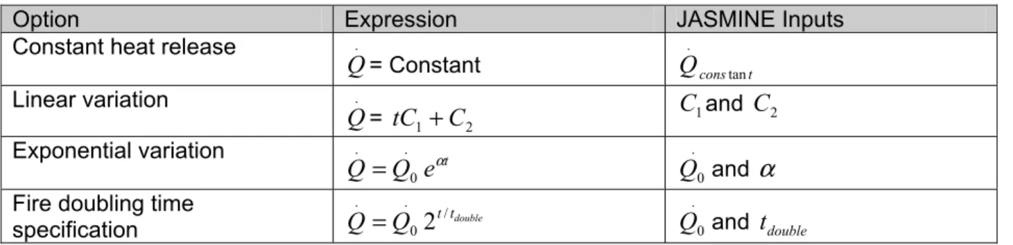
4.3.2 Fire specification

JASMINE provides four different options for specification of the heat release rate: • Constant heat release rate: A single rate is used over the specified time interval. • Linear variation of the heat release rate: the heat varies linearly between the first and

last time step.

• An exponential variation: the rate varies exponentially over the given time step. • The fire doubling time. This option allows the user to provide a time interval over

which the heat release rate doubles.

The expression used by JASMINE to evaluate the heat release rate are summarised in

Table 3.

Table 3. Heat Release Rate Specification Options

Option Expression JASMINE Inputs

Constant heat release .

Q

= Constant Q_cons_tan_t

. Linear variation .

Q

= tC₁ +C₂ C1and C2 Exponential variation _t e Q Q α . 0 . = Q.0and

α

Fire doubling time

specification Q Q t/tdouble . 0 . 2 = Q.0and

t

double 4.4 Conclusions

Field models presented in this section treat turbulence phenomena differently. Either they use Reynolds-Averaged Navier-Stokes (RANS) models or Large Eddy Simulation (LES) models. The model users supply the heat release rate. Each model implements different fire growth methods to estimate the heat release rate. These models are based on an approach that divides an enclosure into a large number of elemental volumes and are considered a micro approach of the fire modeling problem. Computer technology is advancing rapidly. Therefore the use of the field model is increasing and today most of the field models are running on personal computers. However, the execution time of the field model on personal computers is still very high.

Literature Review on the Modeling of Fire Growth and Smoke Movement

Publisher’s version / Version de l'éditeur:

Research Report (National Research Council of Canada. Institute for Research in

Construction), 2003-08-28

Archives des publications du CNRC