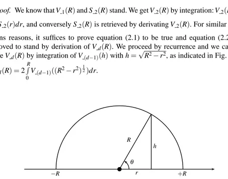
Spheres Unions and Intersections and Some of their Applications in Molecular Modeling
Texte intégral
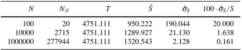
Figure
Documents relatifs
However, our focus in this thesis was on the geometric (gravitational) aspects of the topological defects, wiggly string (in cosmology) and hyperbolic discli- nation (in nematic
L’archive ouverte pluridisciplinaire HAL, est destinée au dépôt et à la diffusion de documents scientifiques de niveau recherche, publiés ou non, émanant des
In Chapter 5, we study the Hecke algebras associated to Kac-Moody groups over local fields.. In Chapter 6, we prove the
Carbon paste electrode modified with carbamoylphosphonic acid functionalized mesoporous silica: A new mercury-free sensor for uranium detection. Factors
Generalization of the equations of crystalline and molecular vibrations in their general rectilinear coordinate axes.. Particular case
In this article, we consider planar graphs in which each vertex is not incident to some cycles of given lengths, but all vertices can have different restrictions. This generalizes
A noteworthy feature of many of the low-voltage discharges in highly conducting liquids is an approximately linear (ohmic) current-voltage behaviour at low-voltage which transitions
A graph G admits an arithmetic sumset labelling f if and only if for any two adjacent vertices in G, the deterministic ratio of every edge of G is a positive integer, which is less
