Publisher’s version / Version de l'éditeur:
Vous avez des questions? Nous pouvons vous aider. Pour communiquer directement avec un auteur, consultez la première page de la revue dans laquelle son article a été publié afin de trouver ses coordonnées. Si vous n’arrivez pas à les repérer, communiquez avec nous à [email protected].
Questions? Contact the NRC Publications Archive team at
[email protected]. If you wish to email the authors directly, please see the first page of the publication for their contact information.
https://publications-cnrc.canada.ca/fra/droits
L’accès à ce site Web et l’utilisation de son contenu sont assujettis aux conditions présentées dans le site LISEZ CES CONDITIONS ATTENTIVEMENT AVANT D’UTILISER CE SITE WEB.
Proceedings of eSim 2018, the 10th conference of IBPSA-Canada, Montréal, QC,
Canada, May 9-10, 2018, 2018-05
READ THESE TERMS AND CONDITIONS CAREFULLY BEFORE USING THIS WEBSITE. https://nrc-publications.canada.ca/eng/copyright
NRC Publications Archive Record / Notice des Archives des publications du CNRC :
https://nrc-publications.canada.ca/eng/view/object/?id=e81253ef-c153-4048-9a23-925884825667
https://publications-cnrc.canada.ca/fra/voir/objet/?id=e81253ef-c153-4048-9a23-925884825667
NRC Publications Archive
Archives des publications du CNRC
This publication could be one of several versions: author’s original, accepted manuscript or the publisher’s version. / La version de cette publication peut être l’une des suivantes : la version prépublication de l’auteur, la version acceptée du manuscrit ou la version de l’éditeur.
Access and use of this website and the material on it are subject to the Terms and Conditions set forth at
Using building performance simulation for fault impact evaluation
Using Building Performance Simulation for Fault Impact Evaluation
Zixiao Shi, William O’Brien
Department of Civil and Environmental Engineering
Carleton University, Ottawa Canada
Abstract: Automated building fault detection and diagnostics (AFDD) has become a valuable tool to maintain the efficiency of high-performance buildings. Still, when faults are detected or diagnosed, they are often presented to the building operators as-is with little explanation of their potential impacts. This could lead to higher workload and knowledge requirement for the operators to assess the situation and schedule maintenance tasks. One approach to aid the building operators’ decision-making process is to provide quantitative impact metrics for faults. Metrics such as energy, thermal comfort, and cost can be simulated using building performance simulation (BPS) software or data-driven models. While BPS has been used in fault detection research as well as advanced control algorithms, little work has done to introduce BPS to fault evaluation and fault management applications. This paper proposes a standardized procedure to use BPS to evaluate diagnosed faults in building systems by quantifying symptoms caused by faults, and then translate these symptoms to BPS inputs. This research tries to tackle the challenges of uncertainties caused by parameter estimation and providing strategies to symptoms that cannot be directly translated to a BPS input. The proposed method can be generalized to be integrated with existing FDD tools or future FDD research.
Keywords: building performance simulation, fault detection and diagnostics, fault evaluation, building energy management
I
NTRODUCTION
Buildings often operate below optimal conditions, which can lead to energy waste, discomfort or even safety hazards (TIAX LLC, 2005). These unpermitted deviations from normal operations in engineering systems are called faults (Isermann, 2006). Severe faults can lead to failures, malfunctions or even safety hazards. According to Isermann (2006), there exist many types of faults, such as design faults, manufacturing faults, normal operation fault (wear and tear), wrong operation fault, maintenance fault, operator’s fault, hardware fault and software fault. There are many approaches to minimize the effects of faults in engineering systems. We can decrease the possibility of a fault occurring by employing more robust design, better manufacturing, and by applying prognostics to predict fault risks. In the domain of buildings, these preventative approaches are usually limited to individual equipment of heating, ventilation, and air conditioning (HVAC) systems. Examples include fault tolerant HVAC control (Wang & Chen, 2002), self-correcting HVAC controls (Cort & Cho, 2011), and robust chillers (Gao, Wang, & Sun, 2011). We can also mitigate faults by using advanced automated fault detection and diagnosis (AFDD) algorithms, and by adopting better fault management strategies. AFDD of building systems has become a popular topic over the last decade (Kim & Katipamula, 2017), thanks to the development of sensing and computing technologies.
Katipamula and Brambley provided a classic review on the topic in their 2005 papers (Katipamula & Brambley, 2005a, 2005b). A follow-up study on the review published in 2017 surveyed 197 articles on building AFDD research (Kim & Katipamula, 2017), and found that over half of the AFDD methods are based on advanced statistical models or machine learning models.
Researchers developing AFDD methods often overlook their implications on fault management – how to meaningfully present AFDD results to building operators to make decision-making faster, as concluded in the reviews by Katipamula and Brambley (2005a, 2005b). Katipamula and Brambley (2005a, 2005b) proposed to include fault impact assessment in AFDD systems to provide quantitative evaluations to the operators, which can help the operators prioritize their work schedule. Still after a decade, according to the recent survey by Kim and Katipamula (2017), only 28 out of the 197 articles provided fault impact estimations in terms of energy and cost. And more than 80% of the 28 articles report fault impacts associate to individual mechanical equipment such as heat pumps and cooling towers. Only O’Neill et al. (2014) included whole building fault impact assessment as part of their study when using EnergyPlus as an anomaly detection tool. There is a lack of research on providing a systematic approach to assess different levels of faults inside building systems.
Interestingly, recent years saw the development of numerous fault models inside building performance
simulation (BPS) tools. For instance, a comprehensive list of fault models was developed with OpenStudio Measures (Cheung & Braun, 2015), and more new fault models are becoming available in EnergyPlus (Zhang & Hong, 2017). Combined with the versatility of BPS tools to change their numerous inputs, this presents a unique opportunity to utilize BPS to simulate and assess fault impacts in buildings in an adaptable manner.
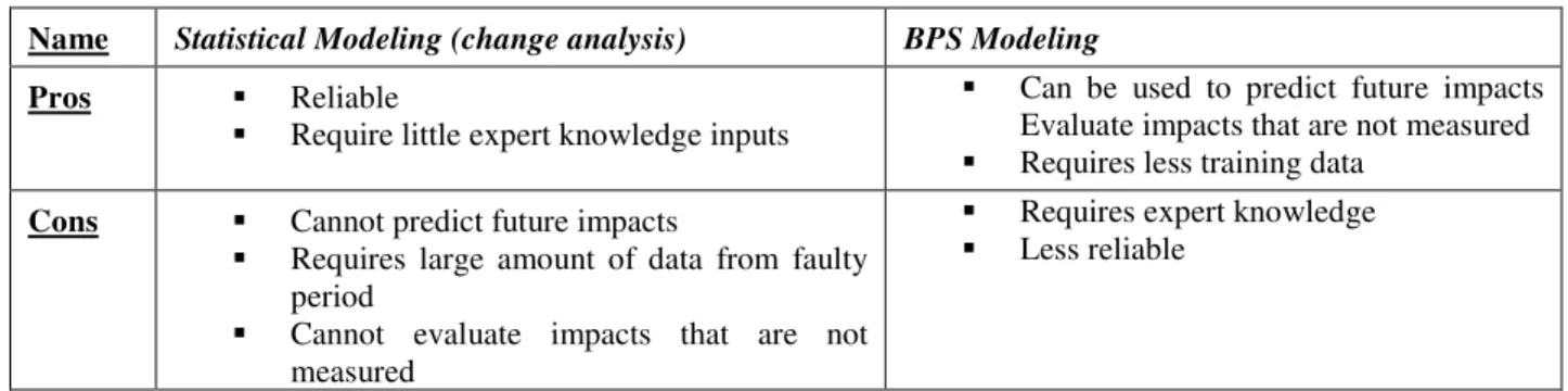
Another approach to evaluating fault impacts is to directly compare measurable metrics before and after the fault. Those methods can be created based on the existing retrofit analysis procedures such as ASHRAE Guideline 14 (ASHRAE, 2014), since they analyze the effect of a change within a system by directly comparing the measured metrics. If the metric of interest is directly observable, this approach can provide reliable analysis. However, it requires sufficient data to be collected after the fault event, which causes conflict with maintenance requirements. In addition, data collected by this approach cannot be used to reliably predict future impacts if the fault is left unresolved. Table 1 shows a comparison between using BPS or statistical model to evaluate fault impacts.
In this paper, the authors favor the usage of BPS tools to evaluate fault impacts. The authors propose a standard procedure for evaluating faults on different scales inside a building, and how to transfer information from sensor readings to BPS model inputs. In addition, a review of existing BPS fault models is provided. We also present a case study as a proof of concept, followed by discussions, future work and a conclusion.
M
ETHODOLOGY
To use BPS tools to assess fault impacts, a baseline model needs to be established for each building. Ideally this model is either passed down from the design stage or created for a previous retrofit analysis. If the baseline model is not available however, it is possible to create calibrated models manually, converted from building information models
(BIM), or optimized from a meta model as proposed by Eisenhower et al. (2012). This paper assumes a baseline model is readily available and will not delve into the process of how to create one.
The challenge of using BPS to evaluate fault impacts is to determine how to quantitatively translate the symptoms caused by a fault to specific inputs inside a BPS model. This involves three major steps:
1. Identify symptoms directly caused by a diagnosed fault. These symptoms will typically cause alterations in building systems, in forms of physical parameter change, availability change or control response change. The causal relationships between symptoms and faults must be defined to achieve this goal. These relationships can be established manually based on first principles and/or obtained through data analytics. The authors reviewed these causal relationships from previous studies and some of them are presented in this paper using qualitative modeling.
2. Quantify severity of the symptom. Since these symptoms are usually deviations from their normal values, this can be achieved through comparing a combination of sensor measurements and estimated parameters to their expected values. This research proposes a quantification approach for both directly and indirectly observed symptoms.
3. Map symptoms to specific inputs in BPS tools. Due to abstractions in different BPS tools, this step heavily relies on expert knowledge. Luckily some fault models have been created with BPS tools during recent years. The authors select some of these mappings in EnergyPlus based on previous research (Mangesh Basarkar, Pang, Wang, Haves, & Hong, 2013; Pang, Wetter, Bhattacharya, & Haves, 2012; Zhang & Hong, 2017) and expert knowledge.
Table 1 Comparison of fault impact evaluation approaches
Name Statistical Modeling (change analysis) BPS Modeling Pros Reliable
Require little expert knowledge inputs
Can be used to predict future impacts Evaluate impacts that are not measured Requires less training data
Cons Cannot predict future impacts
Requires large amount of data from faulty period
Cannot evaluate impacts that are not measured
Requires expert knowledge Less reliable
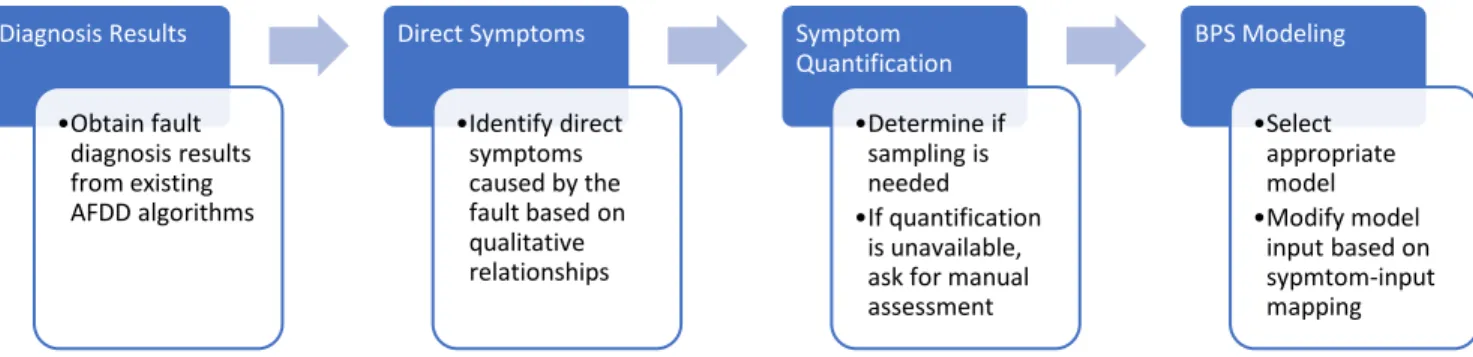
Figure 1 demonstrates the procedure of the proposed method. Details about each step will be further explained in the following sections.
Fault-symptom relationships
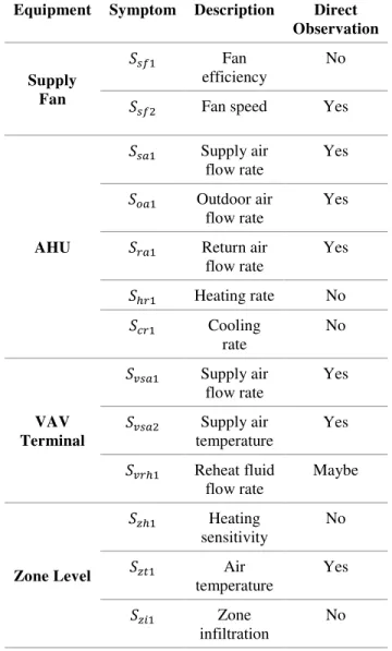
The fault-symptom relationships need to be described both causally and qualitatively. For example, a belt slippage inside a fan will lead to lower fan speed and increased electricity consumption. The relationships developed in this article are based on typical faults and symptoms identified by previous research (Cort & Cho, 2011; Dey & Dong, 2016; Schein, Bushby, Castro, & House, 2006; Xiao, Zhao, Wen, & Wang, 2014; Yu, Woradechjumroen, & Yu, 2014). Table 2 shows a list of symptoms used in this research.
Before the causal relationships are presented, the authors will provide a brief overview of qualitative modeling. We can either use graphical representations (Daigle, 2008) or algebraic representations (Forbus, 1984) for qualitative causal relationships. The authors chose algebraic representation due to its simplicity. Since faults are usually described as discrete states such as fault-free and faulty or negative, neutral and positive; and the physical symptoms are connected to a continuous variable such as temperature and pressure, qualitative influence is used to describe their relationships:
� + (�, �) (1)
� denotes the there exists an influence between � and �, and the + sign indicates the direction of this influence. To further illustrate, this means symptom � is positively influenced by fault �, i.e. a more positive fault � makes symptom � increase in the positive direction. Conversely, negative influence and undetermined influence can be presented by:
� − (�, �) (2)
� ± (�, �) (3)
To further illustrate, the relationship between the previously mentioned fan belt slippage (��1) fault and increased fan electricity usage (��1) can be presented by:
� + (��1,��1)
On the other hand, when the fan is failing (���1), the expected usage of fan electricity will decrease, causing it to move towards the negative direction:
� − (��1,���1)
For a thorough introduction about qualitative process modeling, the classic thesis on this topic by Forbus (1984) can be referenced. If graphical representation is used instead, the thesis by Daigle (2008) can be referred. Table 3 shows examples of some typical faults and symptoms in air handling unit (AHU) and variable air volume (VAV) terminal faults using qualitative influence relationships described above. These tables are far from comprehensive due to length requirements in this paper. A more comprehensive list will be provided as a follow-up study of this paper.
Quantifying a symptom
There are two types of symptoms to be quantified, directly observable and indirectly estimated. Direct observations usually come from the building automation system and human operator inputs, such as sensor readings, control inputs, schedules and visual observations. Indirect estimated symptoms are parameters obtained from first principle and empirical equations, such as chiller efficiency calculated by the ratio between chilled water supply energy and electricity usage. Table contains the information if a symptom is directly observed or not. The observability of the symptoms is shown in Table 2.
Directly observable symptoms can usually be translated to a BPS input using its raw value. This process only requires collecting the corresponding observations after the fault,
Diagnosis Results •Obtain fault diagnosis results from existing AFDD algorithms Direct Symptoms •Identify direct symptoms caused by the fault based on qualitative relationships Symptom Quantification •Determine if sampling is needed •If quantification is unavailable, ask for manual assessment BPS Modeling •Select appropriate model •Modify model input based on sypmtom-input mapping
and then use the mean values of these symptoms to alter the parameter inputs in an EnergyPlus idf file.
To quantify the severity of a symptom that is not directly observed, some form of uncertainty analysis is required. This is due to the uncertainty from modeling applied in this process. This uncertainty analysis can be achieved through sampling. Theoretically, a large number of samples need to be drawn from the collected data to achieve a higher confidence. However, in this application, the approximate range of the fault impact is more of interest. In this case, certain fixed percentiles can be drawn from the collected data to establish this range of fault impacts. In this paper, the three quartiles of 25%, 50% and 75% are used to establish this uncertainty range. Thus, three simulations are performed to evaluate faults with uncertainties.
Multi-level approach to simulation
Building systems operate at different scales, for example a VAV terminal only has effect on the zone it conditions, and faults can propagate through the hierarchy of building systems, i.e. a fault in the AHU can affect all the zones it conditions. It is intuitive to simulate faults at various levels of detail. For example, it is unnecessary to use a whole building model when a fault is only affecting a certain thermal zone. Thus, before mapping the symptoms into BPS inputs, the level of simulation needs to be defined in order to use an appropriate model. The authors define three levels of simulation for fault evaluation: zone level, AHU level and building level. As its name suggests, zone level simulation only uses a zone model to evaluate faults contained within a thermal zone; AHU level is responsible for faults inside an air handling unit affecting all the zones it conditions; and building level faults require the highest order of simulation which affects the performance of a whole building, such as hot water loop faults. The specific definition of which level is required to be simulated will be defined inside the symptom-BPS input mapping section.
Table 2 Example of typical symptoms in building systems
Equipment Symptom Description Direct Observation Supply Fan ���1 Fan efficiency No ���2 Fan speed Yes
AHU ���1 Supply air flow rate Yes ���1 Outdoor air flow rate Yes ���1 Return air flow rate Yes �ℎ�1 Heating rate No ���1 Cooling rate No VAV Terminal ����1 Supply air flow rate Yes ����2 Supply air temperature Yes ���ℎ1 Reheat fluid flow rate Maybe Zone Level ��ℎ1 Heating sensitivity No ���1 Air temperature Yes ���1 Zone infiltration No
Since AFDD is a time sensitive task, it is equally important to provide fault evaluations to the operators in a timely manner. This requires short simulation time of the BPS models.
For zone-level simulation this is easily achievable, however, for AHU-level or building-level models, some form of model order reduction is required to achieve faster simulation time.
There are multiple approaches to BPS model order reduction; the most common one is using surrogate models. This usually requires the training of a black-box model to cover the parameter space of interest, in this case, the parameter space would contain all the potential fault inputs. Examples of this BPS model order reduction approach
include a surrogate model developed in OpenStudio (J. Cole, T. Hale, & F. Edgar, 2013), and the use of support vector regression as a surrogate model (Eisenhower et al., 2012). This approach is usually applied in building design optimization. However, for fault evaluation the parameter space could be much larger than a multi-criteria design optimization, this means to train a machine learning model as surrogate requires an enormous amount of simulation to be performed beforehand.
To avoid this, another approach is to selectively eliminate objects in the BPS model so that it approximates the original model. This is usually called selective node elimination in model order reduction research. Compared to surrogate models, this approach requires much less training data, making it more realistic to achieve. Examples of applying selective node elimination in BPS include using graphic theory to simply building geometry (van Treeck & Rank, 2007), and applying Koopman operator to merge similar thermal zones (Eisenhower, Maile, Fischer, & Mezić, 2010). The model order reduction method used in this paper for AHU-level and building-level fault evaluation is called model-reduce-cluster, developed by (Shi & O’Brien, 2017), and is available as open source Python scripts.
Symptom-input mapping in BPS
After the modelling level is selected, the symptoms quantified from the previous steps can be translated into BPS inputs. Most directly observed symptoms can be translated to certain BPS inputs directly, such as AHU supply air pressure, thermostat setpoint, etc. On the other hand, for other symptoms that cannot be translated to BPS inputs, an indirect mapping approach need to be used. Examples of direct and indirect mappings are shown in Table 4. This indirect mapping is required for most of the
Table 3 Example of typical faults in building systems
Equipment Fa ult Description Relationship Supply Fan ���1 Belt slippage � + ����1,���1� � + ����2,���1� � − (���1,���1) ���2 Decrease in motor efficiency � + ����1,���1� ���3 Overall failure � − (���1,���1) Heating coil �ℎ�1 Fouling � − (�ℎ�1,�ℎ�1) Cooling coil ���1 Fouling � − (���1,���1) Dampers ���1 Return air damper stuck closed � − (���1,���1) ���2 Outdoor air damper stuck open � + (���1,���1) VAV Terminal ��ℎ�1 Reheat valve stuck closed � − (����2,��ℎ�1) � − (���ℎ1,��ℎ�1) � − (���1,��ℎ�1) ���1 Damper stuck open � + (����1,���1) Zone Level ����1 Thermostat temperature positive offset � − (��ℎ1,����1) ���1 Lighting burn out � − (���1,���1) � − (���2,���1)
Table 4 Examples of symptom mappings to EnergyPlus Symptom Mapping in EnergyPlus Modelling level Direct Mapping ���1 Supply fan total efficiency AHU No ���1 Maximum supply air flow rate AHU Yes �zi1 Design infiltration rate Zone No
symptoms quantified by parameter estimations, since the models used for the parameter estimation process are usually different from the first principle models used in the EnergyPlus model (Shi & O’Brien, 2017).
This challenge of indirect mapping can be achieved by applying a common statistical model to the symptom and the corresponding BPS model input, then use a statistical value as an intermediary to translate the symptom severity to a specific BPS input. The authors use normal distribution to describe these values in terms of mean and standard deviation. In truth, there might be better statistical distributions to describe different variables or parameters. Still, such investigation warrants a separate research. First using data collected during normal operation or commissioned operation, the means �� and standard deviations �� of the symptom values can be established. After a fault is diagnosed, deviations of these indirectly observed values can be descripted using z-score:
� =� − �� �
� (4)
In order to translate the z-score to BPS inputs, the same parameter estimation procedures can be applied to the BPS output, using the calibrated model. This means �� and standard deviations �� of the calibrate BPS input. Then the new BPS input used to evaluate the symptom can be calculated by:
� = ��� + �� (5)
This process allows the mapping of quantitative symptoms that cannot be directly translated to BPS inputs.
In this research, EnergyPlus is chosen as the BPS engine for fault evaluations. Table 4 shows an example of different
1 available at
https://github.com/NREL/OpenStudio-fault-models
symptom mappings, modeling level and if they are directly mapped to EnergyPlus inputs. Besides regular model inputs in EnergyPlus, Cheung & Braun (2015) developed a set of fault models with scripts in OpenStudio. It is published as an open source project1. Its most recent update was
committed in 2017 with a new lighting schedule fault, making it capable of simulating 20 types of faults in total. Zhang & Hong (2017) proposed an approach of modifying EnergyPlus inputs to model faults, with five faults and input mappings defined in the methodology section. These fault models are fairly recent, and more fault models will be added to EnergyPlus to expand its usability in building operation applications (Zhang & Hong, 2017).
C
ASE
S
TUDY
A case study was created to demonstrate the proposed fault evaluation method. A calibrated EnergyPlus model of an academic building located at a Canadian university was chosen, as shown in Figure 2. Four faults of different simulation levels were created, including low hot water supply temperature, low AHU supply fan efficiency, increased infiltration rate due to window leakage and stuck closed reheat valve inside a VAV terminal. Symptom data were collected individually to perform the simulations for fault evaluations. Two metrics, site energy in terms of kWh, and thermal comfort in terms of percentage dissatisfied (PPD), were chosen to quantify the fault impacts.
The reduced models used for evaluating building level and AHU level faults are obtained by using the model-cluster-reduce method. Symptoms of Fault 1 and Fault 4 are directly observable sensor measurements. While symptoms of Fault 2 and Fault 4 requires some form of parameter estimation for quantification, as well as uncertainty analysis in fault evaluation. The supply fan efficiency is
estimated by the ratio between supply air flow rate and fan electric power. To estimate zone infiltration rate with commonly available sensors, zone heating sensitivity to the outdoor temperature was used as a surrogate parameter when quantifying symptom severity.
Table 5 shows the results obtained from the case study. The actual fault impacts are calculated directly from the EnergyPlus models used for generating the dataset used in this case study. Overall the evaluated results are reasonably close to the actual fault impact, all within the same order of magnitude, and could provide more insight for the building operators. The boiler fault, which leads to lowered boiler efficiency and inadequate supply hot water temperature, has overestimated fault impacts of more than 200%. This discrepancy is even higher than faults with indirectly observable symptoms. This could be caused by modelling error introduced by the model reduction process. So if time is not a critical issue when assessing the faults, the original building energy model may be used instead to ensure a higher accuracy. The thermal comfort discrepancy of the VAV reheat valve stuck closed fault is quite significant with a 32% error. This discrepancy can be explained by the addition of an extra layer of thermal comfort modelling on top of energy simulation when calculating comfort impacts. This means fault evaluations on thermal comfort may not be as reliable as energy impacts coming from the BPS engines. Still, in terms of overall cost implications, thermal comfort is still a key factor to be considered.
Assessments of faults with symptoms quantified by empirical parameter estimations provided reasonably well insights into how severe the faults will be, even without applying parameter estimation techniques using nonlinear first-principle models. This is possibly due to the fact that consistent empirical parameters were applied to both the original BPS model as well as the faulty operation data, and the dynamics behind the affected BPS inputs and energy consumption outputs are weakly non-linear or almost linear. In cases where the relationship between the
symptom BPS input and energy response becomes highly non-linear, such as a chiller performance curve, the fault evaluation results may become less reliable.
D
ISCUSSION
The method developed in this paper still uses manual mapping of fault-symptom and symptom-BPS input for fault evaluation. Although these mappings are often shared between different building system configurations, they still may become outdated as building systems develop or BPS tools update. As cloud computing and internet of things develop, given enough data in the future containing both normal operation data and faulty operation data of a vast amount of buildings, it may be possible to use pure black-box models instead of analytical simulation to approach the fault evaluation problem. This will be made further possible by the recent development of deep learning and reinforcement learning. However, contrary to recent advancement in AI, which often solves perfect information problems, fault diagnosis and fault evaluation are imperfect information problems since there are variations of sensing capabilities, system configurations and usages from different buildings. An intelligent agent built purely on black-box models, capable of providing reasonable fault evaluations for every kind of building characteristics, is possible but still requires many years of data accumulation and research.
In this research EnergyPlus is chosen as the engine for fault evaluation due to its popularity, and its recent development of fault models. However, there are some inherent issues with EnergyPlus’ capability to simulate faults’ impact on dynamic systems. Firstly, there is a lack of an artificial sensoring layer in EnergyPlus, as all control inputs are directly mapped to an analytical model, and faults such as sensor biases will not be reflected when reporting these readings from simulation. Secondly, there is a lack of real proportional-integral-derivative (PID) control inside EnergyPlus, causing unrealistic response of many
Table 5 Results of evaluated faults in case study
Faults
Energy (kWh) Comfort (PPD) Actual Evaluated Actual Evaluated
1 Boiler low air intake 17,660 47,838 / /
2 AHU supply fan motor deterioration 39,803 48,286-51,078 / /
3 Zone window leakage 1,450 1,016-1,577 / /
engineering systems. These issues can be circumvented by manipulating the energy management system (EMS) scripts, or using co-simulators such as building virtual control test bed (BCVTB). These methods, however, require significant extra work and knowledge. Some other simulation tools, such as ESP-r, do have better control layers when simulating mechanical systems, but are less popular than EnergyPlus and often lack BIM translation capability, making obtaining a calibrated baseline model more difficult.
Besides quantifiable metrics, other potential applications of fault evaluation using BPS include assessing the impact of faults when applying model predictive controls or performing future maintenance actions. For instance, if during the winter a window opening fault is diagnosed but is flagged as low priority due to the size of the room it affects. However, if a heating system shut down is planned, and this future action is simulated along with the diagnosed fault, potential damage caused by freezing can be foreseen and avoided.
CONCLUSIONS
This paper introduces a novel method for exploiting existing BPS tools to assess the impacts of diagnosed faults in building by quantifying and mapping symptoms related to the diagnosed faults to individual BPS model inputs. The proposed framework is scalable to different level of faults inside various building systems. It is applicable to both directly observable symptoms and indirectly estimated symptoms. A case study was created as a proof of concept to demonstrate the usage of the proposed framework. Even though this is still an early stage of readily making this tool available for commercial applications, reviews from previous research and the results from this case study demonstrated the potential benefits of providing quantitative assessments of faults to the building operators by integrating existing BPS technologies.
A
CKNOWLEDGEMENT
The authors of this paper would like to thank Autodesk Research for funding this research. The corresponding author would also like to thank ASHRAE for their support in continuing this work.
R
EFERENCES
ASHRAE. (2014). ASHRAE Guideline 14-2014:
Measurement of Energy , Demand , and Water Savings.
Cheung, H., & Braun, J. E. (2015). Development of Fault
Models for Hybrid Fault Detection and Diagnostics Algorithm Development of Fault Models for Hybrid
Fault Detection and Diagnostics Algorithm.
Cort, K. a, & Cho, H. (2011). Final Project Report : Self-Correcting Controls for VAV System Faults Filter / Fan / Coil and VAV Box Sections, (May).
Daigle, M. J. (2008). A Qualitative Event Based Approach
to Fault Diagnosis of Hybrid Systems. Vanderbilt
University. Vanderbilt University.
https://doi.org/10.1017/CBO9781107415324.004 Dey, D., & Dong, B. (2016). A probabilistic approach to
diagnose faults of air handling units in buildings.
Energy and Buildings, 130, 177–187.
https://doi.org/10.1016/j.enbuild.2016.08.017 Eisenhower, B., Maile, T., Fischer, M., & Mezić, I. (2010).
Decomposing Building System Data for Model Validation and Analysis Using the Koopman Operator. In SimBuild 2010 (pp. 434–441). Retrieved from
http://www.engineering.ucsb.edu/~mgroup/wiki/ima
ges/a/a8/SB10-DOC-TS08B-03-Eisenhower.pdf%5Cnpapers2://publication/livfe/id/ 53095
Eisenhower, B., O’Neill, Z., Narayanan, S., Fonoberov, V. A., & Mezić, I. (2012). A methodology for meta-model based optimization in building energy meta-models.
Energy and Buildings, 47(April), 292–301.
https://doi.org/10.1016/j.enbuild.2011.12.001 Forbus, K. D. (1984). Qualitative Process Theory.
MassaChusetts Institute of Technology, Boston, MA. Gao, D. C., Wang, S., & Sun, Y. (2011). A fault-tolerant and energy efficient control strategy for primary-secondary chilled water systems in buildings. Energy
and Buildings, 43(12), 3646–3656.
https://doi.org/10.1016/j.enbuild.2011.09.037 Isermann, R. (1995). Model Based Fault Detection And
Diagnosis Methods. In Proceedings of the American
Control Conference (pp. 1605–1609).
Isermann, R. (2006). Fault-diagnosis systems: An
introduction from fault detection to fault tolerance. Springer. https://doi.org/10.1007/3-540-30368-5
J. Cole, W., T. Hale, E., & F. Edgar, T. (2013). Building energy model reduction for model predictive control using OpenStudio. In American Control Conference
(ACC) (pp. 449–454).
https://doi.org/10.1109/ACC.2013.6579878
Katipamula, S., & Brambley, M. (2005a). Review Article: Methods for Fault Detection, Diagnostics, and Prognostics for Building Systems—A Review, Part I.
HVAC&R Research, 11(1), 169–187.
https://doi.org/10.1080/10789669.2005.10391133 Katipamula, S., & Brambley, M. (2005b). Review Article:
Methods for Fault Detection, Diagnostics, and Prognostics for Building Systems—A Review, Part II. HVAC&R Research, 11(2), 169–187.
https://doi.org/10.1080/10789669.2005.10391133 Kim, W., & Katipamula, S. (2017). A review of fault
detection and diagnostics methods for building systems. Science and Technology for the Built
Environment, (0), 1–19.
https://doi.org/10.1080/23744731.2017.1318008 Mangesh Basarkar, Pang, X., Wang, L., Haves, P., & Hong,
T. (2013). Modeling and simulation of HVAC faults in EnergyPlus. IBPSA Building Simulation, 14–16.
Retrieved from http://escholarship.org/uc/item/9ps43482.pdf
O’Neill, Z., Pang, X., Shashanka, M., Haves, P., & Bailey, T. (2014). Model-based real-time whole building energy performance monitoring and diagnostics.
Journal of Building Performance Simulation, 7(2),
83–99.
https://doi.org/10.1080/19401493.2013.777118 Pang, X., Wetter, M., Bhattacharya, P., & Haves, P. (2012).
A framework for simulation-based real-time whole building performance assessment. Building and
Environment, 54, 100–108.
https://doi.org/10.1016/j.buildenv.2012.02.003 Schein, J., Bushby, S. T., Castro, N. S., & House, J. M.
(2006). A rule-based fault detection method for air handling units (APAR). Energy and Buildings,
38(12), 1485–1492.
https://doi.org/10.1016/j.enbuild.2006.04.014 Shi, Z., & O’Brien, W. (2017). Building energy model
reduction using model-cluster-reduce pipeline.
Journal of Building Performance Simulation.
https://doi.org/10.1080/19401493.2017.1410572 TIAX LLC. (2005). Energy Impact of Commercial
Building Controls and Performance Diagnostics : Market Characterization, Energy Impact of Building Faults and Energy Savings Potential. Cambridge,
MA USA.
van Treeck, C., & Rank, E. (2007). Dimensional reduction of 3D building models using graph theory and its application in building energy simulation.
Engineering with Computers, 23(2), 109–122.
https://doi.org/10.1007/s00366-006-0053-7
Wang, S., & Chen, Y. (2002). Fault-tolerant control for outdoor ventilation air flow rate in buildings based on neural network. Building and Environment, 37(7), 691–704. https://doi.org/10.1016/S0360-1323(01)00076-2
Xiao, F., Zhao, Y., Wen, J., & Wang, S. (2014). Bayesian network based FDD strategy for variable air volume terminals. Automation in Construction, 41, 106–118. https://doi.org/10.1016/j.autcon.2013.10.019 Yu, Y., Woradechjumroen, D., & Yu, D. (2014). A review
of fault detection and diagnosis methodologies on air-handling units. Energy and Buildings, 82, 550–
562. https://doi.org/10.1016/j.enbuild.2014.06.042 Zhang, R., & Hong, T. (2017). Modeling of HVAC
operational faults in building performance simulation. Applied Energy, 202, 178–188.
https://doi.org/10.1016/j.apenergy.2017.05.153
View publication stats View publication stats