Astronomy& Astrophysics manuscript no. ms ESO 2019c June 12, 2019
Transient processing and analysis using AMPEL: Alert
Management, Photometry and Evaluation of Lightcurves
J. Nordin
1, V. Brinnel
1, J. van Santen
2, M. Bulla
3, U. Feindt
3, A. Franckowiak
2, C. Fremling
4, A. Gal-Yam
5,
M. Giomi
1, M. Kowalski
1, 2, A. Mahabal
4, 6, N. Miranda
1, L. Rauch
2, S. Reusch
1, M. Rigault
7, S. Schulze
5,
J. Sollerman
3, 8, R. Stein
2, O. Yaron
5, S. van Velzen
9, and C. Ward
91 Institute of Physics, Humboldt-Universität zu Berlin, Newtonstr. 15, 12489 Berlin, Germany 2 Deutsches Elektronen-Synchrotron, D-15735 Zeuthen, Germany
3 The Oskar Klein Centre, Department of Physics, Stockholm University, AlbaNova, SE-106 91 Stockholm, Sweden 4 Division of Physics, Mathematics, and Astronomy, California Institute of Technology, Pasadena, CA 91125, USA 5 Department of Particle Physics and Astrophysics, Weizmann Institute of Science 234 Herzl St., Rehovot, 76100, Israel 6 Center for Data Driven Discovery, California Institute of Technology, Pasadena, CA 91125, USA
7 Université Clermont Auvergne, CNRS/IN2P3, Laboratoire de Physique de Clermont, F-63000 Clermont-Ferrand, France 8 Department of Astronomy, Stockholm University, AlbaNova, SE-106 91 Stockholm, Sweden
9 Department of Astronomy, University of Maryland, College Park, MD 20742, USA
June 12, 2019
ABSTRACT
Context.Both multi-messenger astronomy and new high-throughput wide-field surveys require flexible tools for the selection and
analysis of astrophysical transients.
Aims.We here introduce the Alert Management, Photometry and Evaluation of Lightcurves (AMPEL) system, an analysis framework
designed for high-throughput surveys and suited for streamed data. AMPEL combines the functionality of an alert broker with a generic framework capable of hosting user-contributed code, that encourages provenance and keeps track of the varying information states that a transient displays. The latter concept includes information gathered over time and data policies such as access or calibration levels.
Methods.We describe a novel ongoing real-time multi-messenger analysis using AMPEL to combine IceCube neutrino data with the
alert streams of the Zwicky Transient Facility (ZTF). We also reprocess the first four months of ZTF public alerts, and compare the yields of more than 200 different transient selection functions to quantify efficiencies for selecting Type Ia supernovae that were reported to the Transient Name Server (TNS).
Results.We highlight three channels suitable for (1) the collection of a complete sample of extragalactic transients, (2) immediate
follow-up of nearby transients and (3) follow-up campaigns targeting young, extragalactic transients. We confirm ZTF completeness in that all TNS supernovae positioned on active CCD regions were detected.
Conclusions.AMPEL can assist in filtering transients in real time, running alert reaction simulations, the reprocessing of full datasets
as well as in the final scientific analysis of transient data. This is made possible by a novel way to capture transient information through sequences of evolving states, and interfaces that allow new code to be natively applied to a full stream of alerts. This text also introduces how users can design their own channels for inclusion in the AMPEL live instance that parses the ZTF stream and the real-time submission of high quality extragalactic supernova candidates to the TNS.
1. Introduction
Transient astronomy has traditionally used optical telescopes to detect variable objects, both within and beyond our Galaxy, with a peak sensitivity for events that vary on weekly or monthly timescales. This field has now entered a new phase in which multi-messenger astronomy allows for near real-time detec-tions of transients through correladetec-tions between observadetec-tions of different messengers. The initial report of GW170817 from LIGO/VIRGO, and the subsequent search and detection of an X-ray/optical counterpart, provides a first, inspiring example of this (Abbott et al. 2017). Shortly after, the observation of a flar-ing blazar coincident with a high-energy neutrino detected by IceCube illustrated again the scientific potential of time domain multi-messenger astronomy (IceCube Collaboration et al. 2018). Optical surveys now observe the full sky daily, to a depth which encompasses both distant, bright objects and nearby, faint ones. We can thus simultaneously find rare objects, obtain an account-ing of the variable Universe, and probe fundamental physics at
scales beyond the reach of terrestrial accelerators. Exploiting these opportunities is currently constrained as much by software and method development as by available instruments (Allen et al. 2018).
The plans for the Large Synoptic Survey Telescope (LSST) provide a sample scale for high-rate transient discovery. LSST is expected to scan large regions of the sky to great depth, with sufficient cadence for more than 106 astrophysical transients to be discovered each night. Each such detection will be imme-diately streamed to the community as an alert. The challenge of distributing this information for real-time follow-up observa-tions is to be solved through a set of brokers, which will receive the full data flow and allow end-users to select the small subset that merits further study (Juri´c et al. 2017). Development first started on the Arizona-NOAO Temporal Analysis and Response to Events System (ANTARES), which provides a system for real-time characterization and annotation of alerts before they are relayed further downstream (Saha et al. 2014). Other
rent brokers include MARS1 and LASAIR (Smith et al. 2019). Earlier systems for transient information distribution include the Central Bureau for Astronomical Telegrams (CBAT), the Gamma-ray Coordinates Network and the Astronomer’s Tele-gram. The Catalina Real-Time Transient Survey was deisgned to make transient detections public within minutes of observa-tion (Drake et al. 2009; Mahabal et al. 2011). More recent devel-opments include the Astrophysical Multimessenger Observatory Network (AMON, Smith et al. 2013), which provides a frame-work for real-time correlation of transient data streams from dif-ferent high-energy observatories, and the Transient Name Server (TNS), which maintains the current IAU repository for potential and confirmed extragalactic transients2.
While LSST will come online only in 2022, the Zwicky Transient Facility (ZTF) has been operating since March 2018 (Graham 2019). ZTF employs a wide-field camera mounted on the Palomar P48 telescope, and is capable of scanning more than 3750 square degrees to a depth of 20.5 mag each hour (Bellm et al. 2019). This makes ZTF a wider, shallower precursor to LSST, with a depth more suited to spectroscopic follow-up ob-servations. ZTF observations are immediately transferred to the Infrared Processing & Analysis Center (IPAC) data center for processing and image subtraction (Masci et al. 2019). Any sig-nificant point source-like residual flux in the subtracted image triggers the creation of an alert. Alerts are serialized and dis-tributed through a Kafka3 server hosted at the DiRAC centre at University of Washington (Patterson et al. 2019). Each alert con-tains primary properties like position and brightness, but also ancillary detection information and higher-level derived values such as the RealBogus score which aims to distinguish real de-tections from image artifacts (Mahabal et al. 2019). Full details on the reduction pipeline and alert content can be found in Masci et al. (2019), while an overview of the information distribution can be found in the top row of Fig. 3. ZTF will conduct two pub-lic surveys as part of the US NSF Mid-Scale Innovations Pro-gram (MSIP). One of these, the Northern Sky Survey, performs a three-day cadence survey in two bands of the visible Northern Sky.
We here present AMPEL (Alert Management, Photometry and Evaluation of Lightcurves) as a tool to accept, process and re-act to streams of transient data. AMPEL contains a broker as the first of four pipeline levels, or ’tiers’, but complements this with a framework enabling analysis methods to be easily and con-sistently applied to large data volumes. The same set of input data can be repeatedly reprocessed with progressively refined analysis software, while the same algorithms can then also be applied to real-time, archived and simulated data samples. Anal-ysis and reaction methods can be contributed through the im-plementation of simple python classes, ensuring that the vast majority of current community tools can be immediately put to use. AMPEL functions as a public broker for use with the public ZTF alert stream, meaning that community members can pro-vide analysis units for inclusion in the real-time data process-ing. AMPEL also brokers alerts for the private ZTF partnership. Selected transients, together with derived properties, are pushed into the GROWTH Marshal (Kasliwal et al. 2019) for visual ex-amination, discussion and the potential trigger of follow-up ob-servations.
This paper is structured as follows: AMPEL requirements are first described in Sec. 2, after which the design concepts are
pre-1 https://mars.lco.global/ 2 https://wis-tns.weizmann.ac.il/ 3 https://kafka.apache.org
sented in Sec. 3, some specific implementation choices detailed in Sec. 4 and instructions for using AMPEL are provided in Sec. 5. In Sec. 6 we present sample AMPEL uses: systematic reprocess-ing of archived alerts to investigate transient search complete-ness and efficiency, photometric typing and live multi-messenger matching between optical and neutrino data-streams. The dis-cussion (Sec. 7) introduces the automatic AMPEL submission of high-quality extragalactic astronomical transients to the TNS, from which astronomers can immediately find potential super-novae or AGNs without having to do any broker configuration. The material presented here focuses on the design and concepts of AMPEL, and acts as a complement to the software design tools contained in the AMPEL sample repository4. We encourage the in-terested reader to look at this in parallel to this text. We describe the AMPEL system using terms where the interpretation might not match that used in other fields. This terminology will be intro-duced gradually in this text, but is summarized in Table 1 for reference.
2. Requirements
Guided by an overarching goal of analyzing data streams, we here lay out the design requirements that shaped the AMPEL de-velopment:
Provenance and reproducibility: Data provenance encapsu-lates the philosophy that the origin and manipulation of a dataset should be easily traceable. As data volumes grow, and as astronomers increasingly seek to combine ever more diverse datasets, the concept of data provenance will be of central impor-tance. In this era, individual scientists can be expected neither to master all details of a given workflow, nor to inspect all data by hand. As an alternative, these scientists must instead rely on doc-umentation accompanying the data. While provenance is a min-imal requirement for such analysis, a more ambitious goal is re-playability. Replaying an archival transient survey offline would involve providing a virtual survey in which the entire analysis chain is simulated, from transient detection to the evaluation of triggered follow-up observations. In essence, this amounts to an-swering the question: If I had changed my search or analysis pa-rameters, what candidates would have been selected?Because any given transient will only be observed once, replayability is as close to the standard scientific goal of reproducibility as as-tronomers can get.
Analysis flexibility: The next decades will see an unprecedented range of complementary surveys looking for transients through gravitational waves, neutrinos and multiwavelength photons. These will feed a sprawling community of diverse science inter-ests. We would like a transient software framework that is su ffi-ciently flexible to give full freedom in analysis design, while still being compatible with existing tools and software.
Versions of data and software: It is typical that the value of a measurement evolves over time, from a preliminary real-time result to final published data. This is driven both by changes in the quantitative interpretation of the observations, as well as a progressive increase in analysis complexity. The first dimension involves changes such as improved calibration, while the sec-ond incorporates, for example, more computationally expensive
J. Nordin et al.: AMPEL. Alert Management, Photometry and Evaluation of Lightcurves Table 1. AMPEL terminology
Term AMPEL interpretation
Transient Object with a unique ID provided from a data source and accepted into AMPEL by at least one channel.
Datapoint A single measurement with a specific calibration, processing level etc. Compound A collection of datapoints (from one or more instruments).
State A view of a transient object available at some point for some observer. Connects a compound with one (or more) transients.
Tier AMPEL is internally divided into four tiers, where each performs di ffer-ent kinds of operations and is controled by a separate scheduler. Channel Configuration of requested behaviour at all AMPEL tiers supplied by a
user (for one science goal). Typically consists of a list of requested units together with their run parameters.
Archive All alert data, also those rejected during live processing, are stored in an archive for reprocessing.
ScienceRecord Records the result of a science computation made based on data avail-able in specific state.
TransientView All information available regarding a specific transient. This can in-clude multiple states, and any ScienceRecords associated with these. Unit Typically implemented as python modules, a unit allows user
con-tributed code to be directly called during data processing. Units at dif-ferent tiers receive different input and are expected to produce different kinds of output.
Journal A time-ordered log included in each transient.
Purge The transfer of a no longer active transient from the live database to external storage. This includes all connected datapoints, states, com-poundsand ScienceRecords.
Live instance A version of AMPEL processing data in real-time. This includes a number of active channels.
Reprocessing Parsing archived alerts as they would have been received in real-time, using a set of channels defined as for a live instance.
studies only run on subsets of the data. So far it has been hard to study the full impact of incremental changes in these two di-mensions. To change this requires an end-to-end streaming anal-ysis framework where any combinations of data and software can be conveniently explored. A related community challenge is to recognize, reference and motivate continued development of well-written software.
Alert rate: Current optical transient surveys such as DES, ZTF, ASAS-SN and ATLAS, as well as future ones (LSST), do or will provide tens of thousands to millions of detections each night. With such scale, it is impossible for human inspection of all candidates, even assuming that artifacts could be perfectly re-moved5. A simplistic solution to this problem is to only select a very small subset from the full stream, for example a handful of the brightest objects, for which additional human inspection is feasible. A more complete approach would be based on re-taining much larger sets of targets throughout the analysis, from which subsets are complemented with varying levels of follow-up information. As the initial subset selection will by necessity be done in an automated streaming context, the accompanying analysis framework must be able to trace and model these real-time decisions.
5 For optical surveys, a majority of these “detections” are actually
ar-tifacts induced through the subtraction of a reference image. Machine learning techniques, such as RealBogus for ZTF, are increasingly pow-erful at separating these from real astronomical transients. However, this separation can never be perfect and any transient program has to weigh how aggressively to make use of these classifications.
3.
AMPEL
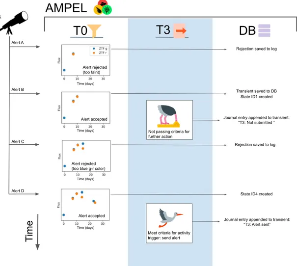
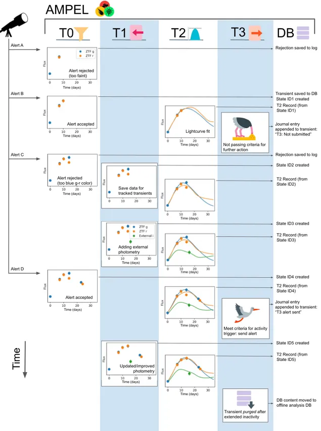
in a nutshellAMPEL is a framework for analyzing and reacting to streamed information, with a focus on astronomical transients. Fulfilling the above design goals requires a flexible framework built using a set of general concepts. These will be introduced in this sec-tion, accompanied by examples based on optical data from ZTF. The “life” of a transient in AMPEL is in parallel outlined in Figs. 1 and 2. These further illustrate many of the concepts introduced in this section. Fig. 1 shows AMPEL used as a straightforward alert broker, while Fig. 2 includes many of the additional features that make AMPEL into a full analysis framework.
The core object in AMPEL is a transient, a single object iden-tified by a creation date and typically a region of origin in the sky. Each transient is linked to a set of datapoints that represent individual measurements6. Datapoints can be added, updated or marked as bad. Datapoints are never removed. Each datapoint can be associated with tags indicating e.g. any masking or pro-prietary restrictions. Transients and datapoints are connected by states, where a state references a compound of datapoints. A state represents a view of a transient available at some time and for some observer. For an optical photometric survey, a com-pound can be directly interpreted as a set of flux measurements or a lightcurve.
Example: A ZTF alert corresponds to a potential transient. Datapoints here are simply the photometric magnitudes reported
6 Note that this is a many-to-many connection; multiple transients can
be connected to the same datapoint due to e.g. positional uncertainty. Datapoints can also originate from different sources.
T0
T3
DB
Alert A Alert B Alert C Alert D Transient saved to DB State ID1 createdJournal entry appended to transient: “T3: Not submitted ”
T
ime
State ID4 created
Journal entry appended to transient: “T3: Alert sent” Rejection saved to log
Rejection saved to log
Time (days) Time (days) Time (days) Time (days)
AMPEL
Alert rejected (too faint) Alert accepted Alert rejected (too blue g-r color)Alert accepted
Not passing criteria for further action
Meet criteria for activity trigger: send alert
Fig. 1. Outline of AMPEL, acting as broker. Four alerts, A to D, belonging to a unique transient candidate are being read from a stream. In a first step, “Tier 0”, the alert stream is filtered based on alert keywords and catalog matching. Alerts B and D are accepted. In a second step, “Tier 3”, it is decided which external resources AMPEL should notify. In this example, only Alert D warrants an immediate reaction. The final column shows the corresponding database events.
by ZTF, which in most cases consists of a recent detection and a history of previous detections or non-detections at this position. When first inserted, a transient has a single state with a com-pound consisting of the datapoints in the initial alert. Should a new alert be received with the same ZTF ID, the new datapoints contained in this alert are added to the collection and a new state is created containing both previous and new data. Should the first datapoint be public but the second datapoint be private, only users with proper access will see the updated state.
Using AMPEL means creating a channel, corresponding to a specific science goal, which prescribes behavior at four different stages, or tiers. What tasks should be performed at what tier can be determined by answers to the questions: “Tier 0: What are the minimal requirements for an alert to be interesting?”, “Tier 1: Can datapoints be changed by events external to the stream?”, “Tier 2: What calculations should be done on each of the candi-dates states?”, “Tier 3: What operations should be done at timed intervals or on populations of transients?”7
– Tier 0 (T0) filters the full alert stream to only include po-tentially interesting candidates. This tier thus works as a
7 Timed intervals include very high frequencies or effectively real-time
response channels.
data broker: objects that merit further study are selected from the incoming alert stream. However, unlike most bro-kers, accepted transients are inserted into a database (DB) of active transients rather than immediately being sent down-stream. All alerts, also those rejected, are stored in an ex-ternal archive DB. Users can either provide their own algo-rithm for filtering, or configure one of the filter classes al-ready available according to their needs.
Example T0: The simple AMPEL channel “BrightAndStable” looks for transients with at least three well behaved detections (few bad pixels and reasonable subtraction FWHM) and not co-incident with a Gaia DR2 star-like source. This is implemented through a python class SampleFilter that operates on an alert and returns either a list of requests for follow-up (T2) anal-ysis, if selection criteria are fulfilled, or False if they are not. AMPEL will test every ZTF alert using this class, and all alerts that pass the cut are added to a DB containing all active tran-sients. The transient is there associated with the channel “Brigh-tAndStable”.
– Tier 1 (T1) is largely autonomous and exists in parallel to the other tiers. T1 carries out duties of assigning datapoints and
J. Nordin et al.: AMPEL. Alert Management, Photometry and Evaluation of Lightcurves
T2 run requests to transient states. Example activities include completing transient states with datapoints that were present in new alerts but where these were not individually accepted by the channel filter (e.g., in the case of lower significance detections at late phases), as well as querying an external archive for updated calibration or adding photometry from additional sources. A T1 unit could also parse previous alerts at or close to the transient position for old data to include with the new detection.
– Tier 2 (T2) derives or retrieves additional transient informa-tion, and is always connected to a state and stored as a Sci-enceRecord. T2 units either work with the empty state, rele-vant for e.g. catalog matching that only depends on the posi-tion, or they depend on the datapoints of a state to calculate new, derived transient properties. In the latter case, the T2 task will be called again as soon as a new state is created. This could be due both to new observations or, for example, updated calibration of old datapoints. Possible T2 units in-clude lightcurve fitting, photometric redshift estimation, ma-chine learning classification, and catalog matching.
Example T2: For an optical transient, a state corresponds to a lightcurve and each photometric observation is represented by a datapoint. A new observation of the transient would extend the lightcurve and thus create a new state.“BrightAndStable” requests a third order polynomial fit for each state using the T2PolyFit class. The outcome, in this case polynomial coef-ficients, are saved to the database.
– Tier 3 (T3), the final AMPEL level, consists of schedulable actions. While T2s are initiated by events (the addition of new states), T3 units are executed at pre-determined times. These can range from yearly data dumps, to daily updates or to effectively real-time execution every few seconds. T3 processes access data through the TransientView, which con-catenates all information regarding a transient. This includes both states and ScienceRecords that are accessible by the channel. T3s iterate through all transients of a channel which were updated since a previous timestamp (either the last time the T3 was run or a specified time-range). This allows for an evaluation of multiple ScienceRecords and comparisons be-tween different objects (such as any kind of population anal-ysis). One typical case is the ranking of candidates which would be interesting to observe on a given night. T3 units include options to push and pull information to and from for example the TNS, web-servers and collaboration communi-cation tools such as Slack8.
Example T3: The science goal of “BrightAndStable” is to observe transients with a steady rise. At the T3 stage the chan-nel therefore loops through the TransientViews, and examines all T2PolyFit science records for fit parameters which indicate a lasting linear rise. Any transients fulfilling the final criteria trigger an immediate notification sent to the user. This test is scheduled to be performed at 13:15 UTC each day.
8 https://slack.com
4. Implementation
We here expand on a selection of implementational aspects. An overview of the live instance processing of the ZTF alert stream can be found in Fig. 3.
Modularity and Units Modularity is achieved through a sys-tem of units. These are python modules that can be incorporated with AMPEL and directly be applied to a stream of data. Units are inherited from abstract classes that regulate the input and out-put data format, but have great freedom in implementing what is done with the input data. The tiers of AMPEL are designed such that each requires a specific kind of information: At Tier 0 the input is the raw alert content, at Tier 2 a transient state, and at Tier 3 a transient view. The system of base classes allows AMPEL to provide each unit with the required data. In a similar system, each unit is expected to provide output data (results) in a spe-cific format to make sure this is stored appropriately: At Tier 0 the expected output is a list of Tier 2 units to run at each state for accepted transients (None for rejected transients). At Tier 2 output is a science record (dictionary) which in the DB is auto-matically linked to the state from which it was derived. The T3 output is not state-bound, but is rather added to the transient jour-nal, a time-ordered history accompanying each transient. Mod-ules at all tiers can make direct use of well developed libraries such as numpy (Oliphant 2006–), scipy (Jones et al. 2001–), and astropy (Astropy Collaboration et al. 2013; Price-Whelan et al. 2018). Developers can choose to make their contributed software available to other users, and gain recognition for functional code, or keep them private. The modularity means that users can inde-pendently vary the source of alerts, calibration version, selection criteria and analysis software.
Schemas and AMPEL shapers Contributed units will be lim-ited as long as they have to be tuned for a specific kind of input, e.g., ZTF photometry. Eventually, we hope that more general code can be written through the development of richer schemas for astronomical information based on which units can be devel-oped and immediately applied to different source streams. The International Virtual Observatory Alliance (IVOA) initiated the development of the VOEvent standard with this purpose9. Core information of each event is to be mapped to a set of specific tags (such as Who, What, Where, When), stored in an XML docu-ment. VOEvents form a starting point for this development (see e.g. Williams et al. 2009), but more work is needed before a general T2 unit can be expected to immediately work on data from all sources. As an intermediate solution, AMPEL employs shapersthat can translate source-specific parameters to a gener-alized data format that all units can rely on. While the internal AMPEL structure is designed for performance and flexibility, it is easy to construct T3 units that export transient information ac-cording to, for example, VOEvent or GCN specifications.
The archive Full replayability requires that all alerts are avail-able at later times. While most surveys are expected to provide this, we keep local copies of all alerts until other forms of access are guaranteed.
9 http:
T0
T1
T2
T3
DB
Alert A Alert B Alert C Alert D Transient saved to DB State ID1 created T2 Record (from State ID1) Journal entry appended to transient: “T3: Not submitted”AMPEL
T
ime
State ID2 created
State ID3 created
State ID4 created
Journal entry appended to transient: “T3 alert sent”
State ID5 created
DB content moved to offline analysis DB Not passing criteria for
further action
Meet criteria for activity trigger: send alert
Transient purged after extended inactivity T2 Record (from State ID2) T2 Record (from State ID3) T2 Record (from State ID4) T2 Record (from State ID5) Rejection saved to log
Rejection saved to log
Time (days) Time (days) Time (days) Time (days) Time (days) Time (days) Time (days) Time (days) Time (days) Time (days) Alert rejected (too faint) Alert accepted Alert rejected (too blue g-r color)
Alert accepted
Save data for tracked transients Adding external photometry Time (days) Updated/improved photometry Time (days) Lightcurve fit
Fig. 2. Life of a transient in AMPEL. Sample behavior at the four tiers of AMPEL as well as the database access are shown as columns, with the left side of the figure indicating when the four alerts belonging to the transient were received. T0: The first and third alerts are rejected, while the second and fourth fulfill the channel acceptance criteria. T1: The first T1 panel shows how the data content of an alert which was rejected at the T0 stage but where the transient ID was already known to AMPEL is still ingested into the live DB. The second panel shows an external datapoint (measurement) being added to this transient. The final T1 panel shows how one of the original datapoints is updated. All T1 operations lead to the creation of a new state. T2: The T2 scheduler reacts every time a new state is created and queues the execution of all T2s requested by this channel. In this case this causes a lightcurve fit to be performed and the fit results stored as a Science Records. T3: The T3 scheduler schedules units for execution at pre-configured times. In this example this is a (daily) execution of a unit testing whether any modified transients warrants a Slack posting (requesting potential further follow-up). The submit criteria are fulfilled the second time the unit is run. In both cases the evaluation is stored in the transient Journal, which is later used to prevent a transient to be posted multiple times. Once the transient has not been updated for an extended time a T3 unit purges the transient to an external database that can be directly queried by channel owners. Database: A transient entry is created in the DB as the first alert is accepted. After this, each new datapoint causes a new state to be created. T2 Science Records are each associated with one state. The T3 units return information that is stored in the Journal.
J. Nordin et al.: AMPEL. Alert Management, Photometry and Evaluation of Lightcurves
Jakob van Santen - Data pipelines for transient astronomy
!18
Live AMPEL instance at DESY
Real-time analysis of Zwicky Transient Facility data
ZTF (Mt. Palomar, California) CalTech, Los Angeles
U. Washington, Seattle >80 exposures/h 47 deg2 each ~350 Mbps 20 detections/s ~2 Mbps data storage
Filtering (T0)
Filtering (T0)
Filtering (T0)
Filtering (Tier 0) Acceptedphotometric points
Filtering (T0)
Filtering (T0)
Filtering (T0)
Light curve analysis(Tier 2)
state storage
NoSQL databases
(Mongo) Population analysis
(Tier 3) Feature calculation task Updated feature Ka fka st re ams (1 6x) Science consumers
Current object states
DESY computing center outside world
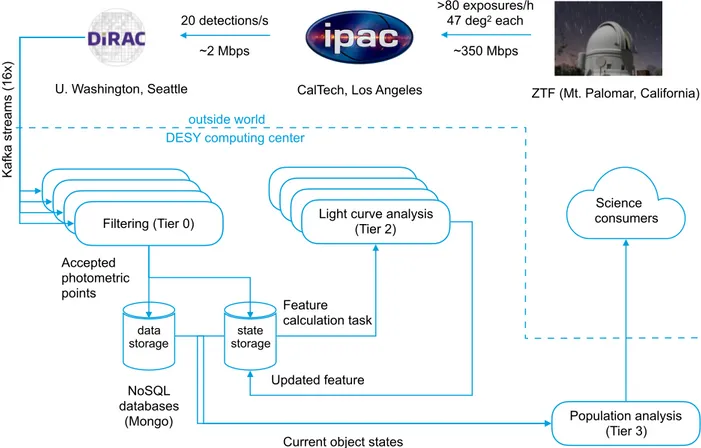
Fig. 3. AMPEL schematic for the live processing of ZTF alerts. External events, above dashed lines: This includes ZTF observations, processing and the eventual alert distribution through the DiRAC centre. Finally, science consumers external to AMPEL receive output information. This can include both full transient display frontends as well as alerts through e.g. TNS or GCN. Internal processing, below dashed line: A set of parallel alert processors examine the incoming Kafka Stream (Tier 0). Accepted alert data is saved into a collection, while states are recorded in another. A light curve analysis (Tier 2) is performed on all states. The available data, including the Tier 2 output, is examined in a Tier 3 unit that selects which transients should be passed out. This particular use case does not contain a Tier 1 stage.
Catalogs, Watch-lists and ToO triggers Understanding astro-nomical transients frequently requires matches to known source catalogs. AMPEL currently provides two resources to this end. A set of large, pre-packaged catalogs can be accessed using catsHTM, including the Gaia DR2 release (Soumagnac & Ofek 2018). As a complement, users can upload their own catalogs using extcats10for either transient filtering or to annotate tran-sients with additional information. extcats is also used to cre-ate watch-lists and ToO channels. Watchlists are implemented as a T0 filter that matches the transient stream with a contributed extcat catalog. A ToO channel has a similar functionality, but employs a dynamic extcat target list where a ToO trigger im-mediately adds one or more entries to the matchlist. The stream can in this case initially be replayed from some previous time (a delayed T0), which allows preexisting transients to be consis-tently detected.
The live database The live transient DB is built using the NoSQL MongoDB11 engine. The flexibility of not having an en-forced schema allows AMPEL to integrate varying alert content and give full freedom to algorithms to provide output of any shape. The live AMPEL instance is a closed system that users can-not directly interact with, and contributed units do can-not directly interact with the DB. Instead, the AMPEL core system manages interactions through the alert, state and transient view objects
10 https://github.com/MatteoGiomi/extcats 11 https://docs.mongodb.com/manual/
introduced above12. Each channel also specifies conditions for when a transient is no longer considered “live”. At this point it is purged: extracted from the live DB together with all states, computations and logs, and then inserted into a channel specific offline DB which is provided to the channel owner.
Horizontal scaling AMPEL is designed to be fully parallelizable. The DB, the alert processors and tier controllers all scale hori-zontally such that additional workers can be added at any stage to compensate for changes to the workload. Alerts can be pro-cessed in any order, i.e. not necessarily in time-order.
AMPELinstances and containers An AMPEL instance is created through combining tagged versions of core and contributed units into a Docker (Merkel 2014) image, which is then converted to the Singularity (Kurtzer et al. 2017) format for execution by an unprivileged user. The final product is a unique “container” that is immutable and encapsulates the AMPEL software, contributed units and their dependencies. These can be reused and referenced for later work, even if the host environment changes signifi-cantly. The containers are coordinated with a simple orchestra-tion tool13 that exposes an interface similar to Docker’s “swarm
12 Eventually, daily snapshot copies of the DB will be made available
for users to interactively examine the latest transient information with-out being limited with what was reconfigured to be exported.
mode.” Previously-deployed AMPEL versions are stored, and can be run off-line on any sequence of archived or simulated alerts. Several instances of AMPEL might be active simultaneously, with each processing either a fraction of a full live-stream, or some set of archived or simulated alerts. Each works with a distinct database. The current ZTF alert flow can easily be parsed by a single instance, called the live instance. A full AMPEL analy-sis combines this active parsing and reacting to the live streams with subsequent or parallel runs in which the effects of the chan-nel parameters can be systematically explored.
Logs and provenance AMPEL contains extensive, built-in log-gingfunctions. All AMPEL units are provided a logger, and we recommend this to be consistently used. Log entries are auto-matically tagged with the appropriate channel and transient ID, and are then inserted into the DB. These tools, together with the DB content, alert archive and AMPEL container, make prove-nance straightforward. The IVOA has initiated the development of a Provenance Data Model (DM) for astronomy, following the definitions proposed by the W3C (Sanguillon et al. 2017)14. Sci-entific information is here described as flowing between agents, entities and activities. These are related through causal rela-tions. The AMPEL internal components can be directly mapped to the categories of the IVOA Provenance DM: Transients, data-points, states and ScienceRecords are entities, Tier units are ac-tivities and users, AMPEL maintainers, software developers and alert stream producers are agents. A streaming analysis carried out in AMPEL will thus automatically fulfill the IVOA provenance requirements.
Hardware requirements The current live instance installed at the DESY computer center in Berlin-Zeuthen consists of two machines, “Burst” and “Transit”. Real time alert processing is done at Burst (32 cores, 96 GB memory, 1 TB SSD) while alert reception and archiving is done at Transit (20 cores, 48 GB mem-ory, 1 TB SSD+ medium-time storage). This system has been designed for extragalactic programs based on the ZTF survey, with a few ×105 alerts processed each night, of which between 0.1 and 1% are accepted. Reprocessing large alert volumes from the archive on Transit is done at a mean rate of 100 alerts per sec-ond. As the ZTF live alert production rate is lower than this, and Burst is a more powerful machine, this setup is never running at full capacity. It would be straightforward to distribute process-ing of T2 and T3 tasks among multiple machines, but as the ex-pected practical limitation is access to a common database, this is of limited use until extremely demanding units are requested.
5. Using
AMPEL
5.1. Creating a channel for the ZTF alert stream
The process for creating AMPEL units and channels is fully described in the Ampel-contrib-sample repository15, which also contains a set of sample channel configurations. The steps to implementing a channel can be summarized as follows:
1. Fork the sample repository and rename it Ampel-contrib-groupIDwhere groupID is a string identifying the contribut-ing science team.
14
http://www.ivoa.net/documents/ProvenanceDM/20181015/PR-ProvenanceDM-1.0-20181015.pdf
15 https://github.com/AmpelProject/Ampel-contrib-sample
2. Create units through populating the t0/t2/t3 sub-directories with python modules. Each is designed through inheriting from the appropriate base class.
3. Construct the repository channels by defining their param-eters in two configuration files: channels.json which de-fines the channel name and regulates the T0, T1 and T2 tiers, and t3_jobs.json which determines the schedule for T3 tasks. These can be constructed to make use of AMPEL units present either in this repository, or from other public AMPEL repositories.
4. Notify AMPEL administrators. The last step will trigger chan-nel testing and potential edits. After the chanchan-nel is verified, it will be added in the list of AMPEL contribution units and included in the next image build. The same channel can also (or exclusively) be applied to archived ZTF alerts.
5.2. Using AMPEL for other streams
Nothing in the core AMPEL design is directly tied to the ZTF stream, or even optical data. The only source-specific software class is the Kafka client reading the alert stream, and the alert shapers which make sure key variables such as coordinates are stored in a uniform matter. Using a schema-free DB means that any stream content can be stored by AMPEL for further process-ing. A more complex question concerns how to design units us-able with different stream sources. As an example, different op-tical surveys might use different conventions for how to encode which filter was used, and the reference system and uncertainty of reported magnitudes and powerful alert metrics, such as the RealBogus value of ZTF, are unique. Until common standards are developed, classes will have to be tuned directly to every new alert stream.
6. Initial
AMPEL
applications6.1. Exploring the ZTF alert parameter space
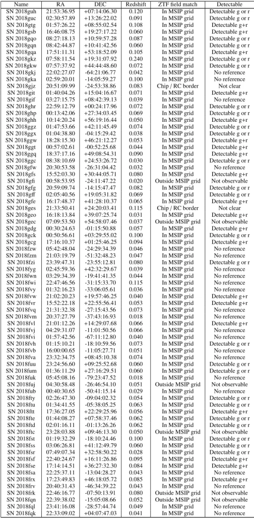
It has been notoriously challenging to quantify transient detec-tion efficiencies, search old surveys for new kinds of transients, and predict the likely yield from a planned follow-up campaign. We here demonstrate how AMPEL can assist with such tasks. For this case study we reprocess 4 months of public ZTF alerts using a set of AMPEL filters spanning the parameter space of the main properties of ZTF alerts. The accepted samples of each channel are, in a second step, compared with confirmed Type Ia super-novae (SNe Ia) reported to the TNS during the same period. We can thus examine how different channel permutations differ in detection efficiency, and at what phase each SN Ia was “discov-ered”. The base comparison sample consists of 134 normal SNe Ia. The creation of this sample is described in detail in Appendix A.
We processed the ZTF alert archive from June 2nd 2018 (start of the MSIP Northern Sky Survey) to October 1st using 90 potential filter configurations based on the DecentFilter class. In total 28667252 alerts were included. Each channel exists on a grid constructed by varying the properties described in Table 2. We also include 24 OR combinations where the accept criteria of two filters are combined. We further consider two additional versions of each filter or filter-combination:
1. Transients in galaxies with known active SDSS or MILLI-QUAS active nuclei (Flesch 2015; Pâris et al. 2017) are re-jected, and
J. Nordin et al.: AMPEL. Alert Management, Photometry and Evaluation of Lightcurves
2. Transients are required to be associated with a galaxy for which there is a known NED or SDSS spectroscopic redshift z< 0.1.
In total, this amounts to 342 combinations. All of these vari-ants include some version of alert rejection based on coinci-dence with a star-like object in either PanSTARRS (using the algorithm of Tachibana & Miller 2018) or Gaia DR2 (Gaia Col-laboration et al. 2018). We also tested channels not including any such rejection, which lead to transient counts around 105 (an order of magnitude greater than with the star-rejection veto). Reprocessing the alert stream in this way took 5 days even in a non-optimized configuration, demonstrating that AMPEL can pro-cess data at the expected LSST alert rate.
This study is neither complete nor unbiased: A large frac-tion of the SNe were classified by ZTF, and we know that the real number of SNe Ia observed is much larger than the classi-fied subset. Nonetheless it serves both as a benchmark test for channel creation, as well as a starting point for more thorough analysis. An estimate of the total number of supernovae we ex-pect to be hidden in the ZTF detections can be obtained through the simsurvey code (Feindt et al. 2019), in which known tran-sient rates are combined with a realistic survey cadence and a set of detection thresholds16. The predicted number of Type Ia supernovae fulfilling the criteria of one or more of these chan-nels over the same timespan as the comparison sample and with weather conditions matching the observed was found to be 1033 (average over 10 simulations). Simsurvey also conveniently re-turns estimates for other supernova types and we find that an additional 276 Type Ibc, 92 Type IIn and 377 Type IIP super-novae are likely to have been observed by ZTF under the same conditions. The total number of supernovae present in the alert sample is thus estimated to be 1778.
The results for channel efficiencies, compared to the total number of accreted transients, can be found in Fig. 4. Though we observe the obvious trend that channels with larger coverage of the comparison sample also accept a larger total number of transients, there is also a variation in the total transient counts between configurations that find the same fraction of the com-parison sample. Fig. 4 highlights a subset of the channels as par-ticularly interesting. Selection statistics for these channels can be found in Table 3. For comparison objects with a well defined time of peak light, we also monitor the phase at which it was accepted into each channel. As an estimate for this we use the time of B-band peak light as determined by a SALT lightcurve fit, which is carried out for each candidate at the T2 tier (Be-toule et al. 2014). This information can be used to study how well channels perform in finding early SNe Ia, which consti-tute a prime target for many supernova science studies. In fig-ure 4 we therefore mark all channels where more than 25% of all SNe Ia were accepted prior to −10 days relative to peak light (“Early detection”). Alternatively, SN Ia cosmology pro-grams often look for a combination of completeness and discov-ery around lightcurve peak to facilitate spectroscopic classifica-tion. Channels not fulfilling the Early detection criteria but where more than 95% of all SNe Ia were accepted prior to peak light are therefore marked as “Peak classification”. These two simple ex-amples highlight how reprocessing alert streams (reruns) can be used to optimize transient programs, and to estimate yields use-ful for e.g follow-up proposals. We also find that a 4% fraction of the comparison sample (5 out of 134) were found in galaxies with documented AGNs, suggesting that programs which
pri-16 https://github.com/ufeindt/simsurvey
oritize supernova completeness cannot reject nuclear transients with active hosts.
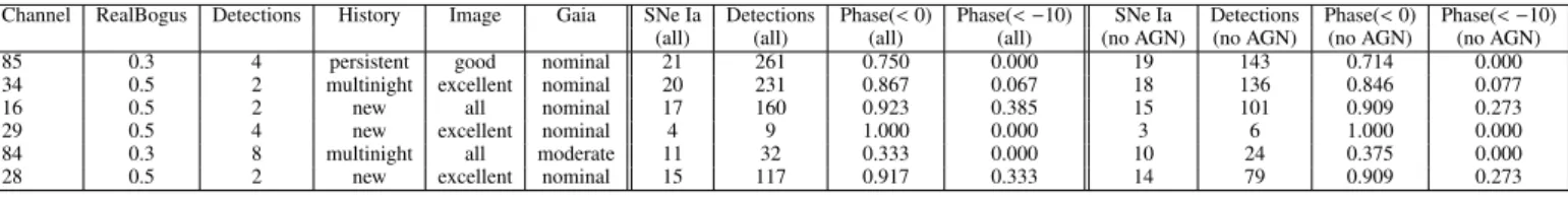
With AMPEL we are getting closer to one main goal of future transient astronomy – the immediate, robotic follow-up of the most interesting detections. Facilities such as LCO, the Liver-pool Telescope and the Palomar P60 now have the instrumental capabilities for robotic triggers and execution of observations. As the next step towards this we also explore how to select can-didates for such automatic programs. Figure 4 (right panel) and Table 4 show channels where only transients in confirmed nearby galaxies are accepted. While total transient and matched SN Ia counts are much reduced here, all remaining transient candidates can be said with high probability to be both extragalactic and nearby, and thus good candidates for follow-up. Channels such as “16” and “28” can here be expected to automatically detect multiple early SNe Ia each year and still have small total counts (160 and 117 transients accepted, respectively).
Based on this exploration we highlight three channels: – Channel 10+ 59, the union of Channels 10 and 59 and
in-cluding AGN galaxies, is the channel which accepts the least amount of transients while recovering the full comparison sample prior to peak light. We will refer to this as the “com-plete”channel.
– Channel 1 (including AGN galaxies) strikes a balance be-tween a relatively high completeness (> 80%) while detect-ing transients early and with a limited number of total ac-cepted transients. As will be discussed in Sec.7.1 this chan-nels performs the initial election for the current automatic candidate submission to TNS and is thus referred to as the “TNS” channel.
– Channel 16, coupled with only accepting transients in nearby non-AGN host galaxies, provides a very pure selection suit-able for automatic follow-up. Consequently, this will be ref-erenced as the “robotic” channel. We add “N” to the chan-nel number (16N) to remind that only transients in nearby (z < 0.1) galaxies are admitted.
The “complete” and “TNS” channels differ mainly in that the first accepts transients closer to Gaia sources.
6.2. Channel content and photometric transient classification The previous section examined channels mainly based on the fraction of a known comparison SN Ia sample which was redis-covered. However, as mentioned, the real number of unclassified supernovae (of all types) will be much larger. Every channel will also contain subsets of all other known astronomical variables (e.g. AGNs, variable stars, solar system objects), still unknown astronomical objects and noise. This gap between photometric detections and the number of spectroscopically classified objects will only increase as the number and depth of survey telescopes increase. Developing photometric classification methods is thus one of the key requisites for the LSST transient program.
ZTF is different in that most transients are nearby and could be classified and the ZTF stream thus provides a way to develop classification methods where the predictions can be verified. As a more immediate application we would like to gain a more gen-eral understanding of what transients the AMPEL channels pro-duce. As a first step in this process we can use the SN Ia template fits introduced in Sec. 6.1 as a primitive photometric classifier. The fits were carried out using a T2 wrapper to the SNCOSMO package17. In this case the run configuration only requested the
Table 2. Dominant channel selection variables and potential settings.
Channel property Options
RealBogus Nominal:Require ML score above 0.3 or Strong: above 0.5 Detections More than [2, 4, 6, 8] (any filter)
Alert History New:Not older than 5 days, Multi-night: 4 to 15 days, Persistent: Older than 8 days.
Image Quality All:No requirements, Good: Limited cuts on e.g. FWHM and bad pix-els, Excellent: Strong cuts on e.g. FWHM and bad pixels.
Gaia DR2 Nominal:Reject likely stars from Gaia DR2, Moderate: only search in small aperture or Disabled.
Star-Galaxy separation Using PS1 star-galaxy separation (Tachibana & Miller 2018) to reject potential stars (Hard), likely stars (Nominal) or no rejection (Disabled). Match confusion Nominal:Allow candidates close to nearby (confused) sources, or
Dis-abled: reject anything close to stars even if other sources exist.
0 0.2 0.4 0.6 0.8 1.0
Efficiency (fraction of TNS SNe Ia detected) 101
102 103 104
Number of transients in channel
SN Ia rate from simulations 11 26 10+59 34 18 77 51 57 64 1 28 4 Early detection Peak classification Any phase
with AGN hosts without AGN hosts
0.0 2.5 5.0 7.5 10.0 12.5 15.0 17.5 20.0 TNS SNe Ia detected
100 101 102
Number of transients in channel
85 34 16 29 84 28
Restricted to transients in known z < 0.1 galaxies Early detection
Peak classification Any phase
Fig. 4. A comparison of the total number of accepted candidates (y-axis) with fraction of the comparison sample SNe Ia detected as x-axis. Symbol shapes indicate the typical phase at which objects in the comparison sample were detected: Channels where more than 25% were detected prior to phase −10 are marked as early (squares). If instead more than 95% were detected prior to peak light the channel is defined as suitable for peak classification (circles). Channels not fulfilling either criteria are marked with triangles. Left panel: Full channel content. Channels are here divided according to those where transients in galaxies known to host AGN are cut (black) and channels where these are accepted (grey). Compare Table 3. Right panel: Comparison of the total number of accepted candidates (y-axis) with the number of comparison sample SNe Ia found, with only candidates linked to a galaxy with known spectroscopic redshift z < 0.1. All channels reject transients in host galaxies with known AGNs. Compare Table 4. Three channels further discussed in the main text are highlighted (red circles).
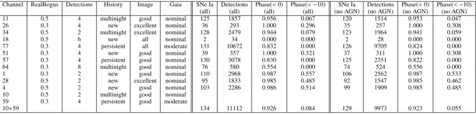
Table 3. AMPEL sample channel parameter settings and rerun statistics. Columns 2 to 6 show settings used for parameters in Table 2, columns 7 to 10 statistics including all targets and columns 11 to 14 repeating these when excluding AGN associated candidates. The phase estimates describe the fraction of the matched SNe Ia with a good peak phase estimate that were accepted by the channel either prior to lightcurve peak or prior to −10 days with respect to peak light.
Channel RealBogus Detections History Image Gaia SNe Ia Detections Phase(< 0) Phase(< −10) SNe Ia Detections Phase(< 0) Phase(< −10) (all) (all) (all) (all) (no AGN) (no AGN) (no AGN) (no AGN) 11 0.5 4 multinight good nominal 125 1857 0.956 0.067 120 1514 0.953 0.047 26 0.3 4 new excellent nominal 36 293 1.000 0.296 35 257 1.000 0.308 34 0.5 2 multinight excellent nominal 128 2479 0.944 0.079 123 1964 0.941 0.059
18 0.5 6 new all nominal 2 34 0.000 0.000 2 28 0.000 0.000
77 0.3 4 persistent all moderate 131 10672 0.832 0.000 126 9705 0.824 0.000
51 0.3 4 new good nominal 39 357 1.000 0.321 37 311 1.000 0.308
57 0.3 4 persistent good nominal 130 3078 0.830 0.000 125 2351 0.822 0.000 64 0.3 8 multinight good nominal 76 580 0.554 0.000 74 524 0.556 0.000 1 0.3 2 new good nominal 110 2968 0.987 0.557 106 2562 0.987 0.533 28 0.5 2 new excellent nominal 95 1833 0.985 0.485 92 1547 0.985 0.462 4 0.5 2 new good nominal 103 2286 0.986 0.514 99 1909 0.985 0.485 10 0.5 2 multinight good nominal
59 0.3 4 persistent good moderate
10+59 134 11112 0.926 0.084 129 9973 0.923 0.055
SALT2 SN Ia model to be included, but any transient template could have been requested. During the stream processing a fit will be done to each state, but we here only analyze the final state fit as we are investigating sample content rather than the evolution of classification accuracy with time (the latter question is more interesting but harder).
Out of the 11112 transients accepted by the complete (10+ 59) channel, 6995 have the minimal number of detections (5) required to fit the SALT2 parameters x1 (lightcurve width), c (lightcurve color), t0 (time of peak light), x0 (peak magnitude) and zphot(redshift from template fit). Further requiring the cen-tral values of the fit parameters to match parameter ranges
ob-J. Nordin et al.: AMPEL. Alert Management, Photometry and Evaluation of Lightcurves
Table 4. AMPEL sample channel parameter settings and rerun statistics for cases when only transients close to z < 0.1 host galaxies are included. Columns 2 to 6 show settings used for parameters in Table 2, columns 7 to 10 statistics including all targets and columns 11 to 14 repeating these when excluding AGN associated candidates. The phase estimates describe the fraction of the matched SNe Ia with a good peak phase estimate that were accepted by the channel either prior to lightcurve peak or to −10 days w.r.t. peak.
Channel RealBogus Detections History Image Gaia SNe Ia Detections Phase(< 0) Phase(< −10) SNe Ia Detections Phase(< 0) Phase(< −10) (all) (all) (all) (all) (no AGN) (no AGN) (no AGN) (no AGN) 85 0.3 4 persistent good nominal 21 261 0.750 0.000 19 143 0.714 0.000 34 0.5 2 multinight excellent nominal 20 231 0.867 0.067 18 136 0.846 0.077
16 0.5 2 new all nominal 17 160 0.923 0.385 15 101 0.909 0.273
29 0.5 4 new excellent nominal 4 9 1.000 0.000 3 6 1.000 0.000
84 0.3 8 multinight all moderate 11 32 0.333 0.000 10 24 0.375 0.000 28 0.5 2 new excellent nominal 15 117 0.917 0.333 14 79 0.909 0.273
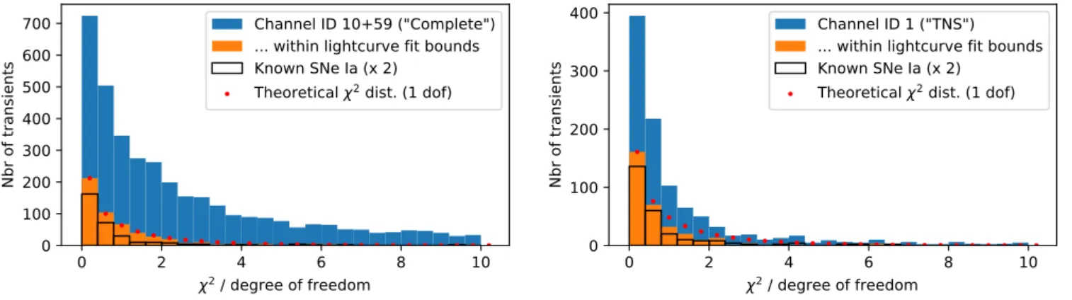
served among nearby SNe Ia (−3 < x1 < 3, −1 < c < 2, 0.001 < zphot < 0.2 and zerr < 0.1) leaves 634 transients. In fig. 5 we compare the distributions of χ2per degree of freedom for these samples. We find that the subset following typical SN Ia parameters match both the expected theoretical fit quality dis-tribution and has a disdis-tribution similar to the values obtained for the comparison sample of spectroscopically confirmed SNe Ia. This “SN Ia compatible” subset can be thus be used as an ap-proximate photometric SN Ia sample18. Repeating this study for the “TNS” channel 1, which accepted 2968 transients, we find that 1342 objects can be fit and that out of these 349 are compat-ible with the standard SN Ia parameter expectations.
We next examine the observed peak magnitudes for both the complete and efficient channels (fig 6). For both channels, the subsets restricted to standard SN Ia parameter ranges agree well with the comparison objects for bright magnitudes (< 18.5 mag). Fainter than this limit both channels contain a large sample of likely SNe Ia with a detection efficiency that rapidly drops be-yond 19.5 mag. Both limits are expected as the ZTF RCF pro-gram attempts to classify all extragalactic transients brighter than 18.5 mag and supernovae peaking fainter than ∼ 19.5 mag often do not yield the five significant measurements that are required to trigger the production of an alert and will thus not be included in the lightcurve fit. Most of these fainter SNe will have several late-time observations below the 5σ threshold that did not trig-ger alerts but which will be recoverable once the ZTF image data is released. We find no significant differences between the com-plete and TNS channels in terms of magnitude coverage, con-sistent with the fact that they differ mainly in that the complete channel accepts transients closer to Gaia sources.
We can thus define two (overlapping) subsets for each chan-nel: The comparison sample of known SN Ia (“Reference SN Ia”) and the photometric SNe Ia (“Photo SN Ia”) with lightcurve fit parameters compatible with a SN Ia. We complement these with five subsets based on external properties:
– Transients that coincide with an AGN in the Million Quasar Catalog or SDSS QSO catalogs are marked as “Known AGN”.
– Transients that coincide with the core of a photometric SDSS galaxy are marked “SDSS core” (distance less than 100). – Transients that coincide with a SDSS galaxy outside the core
are marked “SDSS off-core” (distance larger than 100). – Transients that were reported to the TNS as a likely
extra-galactic transient but do not have a confirmed classification are marked “TNS AT”.
– Transients that do have a TNS classification but are not part of the reference sample of SNe Ia are called “TNS SN (other)”
18 Any algorithm for evaluating photometric data can similarly be
im-plemented as a T2 unit and applied to the same rerun dataset. Transient models that can be incorporated into SNCOSMO can even use the same T2 unit and only vary run configuration.
The count and overlap between these groups are shown in fig. 7. We here only include transients with a peak brighter than 19.5 mag as the fraction with lightcurve fit falls quickly beyond this limit (fig. 6). We can make several observations already based on this crude accounting: For the complete channel these categorizations accounts for 40% of all accepted transients. The remaining fraction consists of a combination of real extragalac-tic transients that were not reported to the TNS, stellar variables not listed in Gaia DR2 and “noise”. For the efficient channel, only 20% of all detections (152 of 771) are in this sense unac-counted for. We observe that large fractions of SNe are found both aligned with the core of SDSS galaxies as well as without association to a photometric SDSS galaxy. This directly demon-strates how care must be taken when selecting targets for surveys looking for complete samples.
A main goal for transient astronomy, and AMPEL, during the coming decade will be to decrease the fraction of unknown tran-sients as much as possible. Machine learning based photometric classification will be essential to this endeavor, but other devel-opments are as critical. These include the possibility to better distinguish image and subtraction noise (“bogus”) and the abil-ity to compare with calibrated catalogs containing previous vari-ability history. We plan to revisit this question once the ZTF data can be investigated for previous or later detections.
6.3. Real-time matching with IceCube neutrino detections The capabilities and flexibility of AMPEL can also be highlighted through the example of the IceCube realtime neutrino multi-messenger program. Several years ago, the IceCube Neutrino Observatory discovered a diffuse flux of high-energy astrophys-ical neutrinos (IceCube Collaboration 2013). Despite recent ev-idence identifying a flaring blazar as the first neutrino source (IceCube Collaboration et al. 2018), the origin of the bulk of the observed diffuse neutrino flux remains, as yet, undiscov-ered. One promising approach to identify these neutrino sources is through multi-messenger programs which explore the pos-sibility of detecting multi-wavelength counterparts to detected neutrinos. Likely high-energy neutrino source classes with opti-cal counterpart are typiopti-cally variables or transients emitting on timescales of hours to months, for example core collapse super-novae, active galactic nuclei or tidal disruption events (Waxman 1995; Atoyan & Dermer 2001, 2003; Farrar & Gruzinov 2009; Murase & Ioka 2013; Petropoulou et al. 2015; Senno et al. 2016; Lunardini & Winter 2017; Senno et al. 2017; Dai & Fang 2017). To detect counterparts on these timescales, telescopes are re-quired which feature a high cadence and a large field-of-view, in order to cover a significant fraction of the sky. In addition to an optimized volumetric survey speed capable of discover-ing large numbers of objects, neutrino correlation studies require robustly-classified samples of optical transient populations. In order to provide a prompt response to selected events within
0
2
4
6
8
10
2/ degree of freedom
0
100
200
300
400
500
600
700
Nbr of transients
Channel ID 10+59 ("Complete")
... within lightcurve fit bounds
Known SNe Ia (x 2)
Theoretical
2dist. (1 dof)
0
2
4
6
8
10
2/ degree of freedom
0
100
200
300
400
Nbr of transients
Channel ID 1 ("TNS")
... within lightcurve fit bounds
Known SNe Ia (x 2)
Theoretical
2dist. (1 dof)
Fig. 5. Histogram of SALT2 SN Ia fit quality (chi2per degree of freedom) for the complete 10+ 59 channel. Blue bars show the full sample (with
enough detections for fit) while orange shows the subset which also fulfill the expected fit parameter requirements. These are compared with with fit quality for the subset of known SN Ia in the comparison sample (outlined bars, scaled with a factor 2) as well as a standard χ2distribution for
one degree of freedom (scaled to match the first bin of the restricted sample ).
14 15 16 17 18 19 20 21
Peak observed magnitude (g)
100 101 102 103Nbr of transients
Channel ID 10+59 ("Complete") ... within lightcurve fit bounds Confirmed SNe Ia14 15 16 17 18 19 20 21
Peak observed magnitude (g)
100101
102
Nbr of transients
Channel ID 1 ("TNS") ... within lightcurve fit bounds Confirmed SNe Ia
Fig. 6. Peak magnitude distributions (ZTF g band) for the same subsets. The comparison sample is not scaled. Left panel: Data for the complete 10+ 59 channel. Right panels: Data for the efficient 1 channel.
Ref. SN Ia TNS SN (other)
TNS AT Photo SNIa
SDSS off-coreSDSS coreKnown AGN
Ref. SN Ia TNS SN (other) TNS AT Photo SNIa SDSS off-core SDSS core Known AGN 178 0 188 0 0 328 125 66 85 446 38 43 53 92 244 35 26 96 78 0 392 4 1 71 11 6 158 242 Ch. ID 10+59 ("Complete") Not matched: 15542761 transients
Ref. SN Ia TNS SN (other)
TNS AT Photo SNIa
SDSS off-coreSDSS coreKnown AGN
Ref. SN Ia TNS SN (other) TNS AT Photo SNIa SDSS off-core SDSS core Known AGN 148 0 118 0 0 173 102 36 45 263 33 28 24 59 128 26 10 43 39 0 173 3 1 28 5 5 51 82 Ch. ID 1 ("TNS") Not matched: 129770 transients
Ref. SN Ia TNS SN (other)
TNS AT Photo SNIa
SDSS off-coreSDSS coreKnown AGN
Ref. SN Ia TNS SN (other) TNS AT Photo SNIa SDSS off-core SDSS core Known AGN 19 0 11 0 0 5 12 4 1 20 8 8 2 11 24 10 2 3 7 0 20 0 0 0 0 0 0 0 Ch. ID 16N ("Robotic") Not matched: 249 transients
Fig. 7. Estimated transient types for objects with a peak magnitude brighter than 19.5 for the channels 10+ 59 (“complete”), 1 (“efficient”) and 16 (“robotic”). The channel 16 selection also requires transients to be close to host galaxies with a spectroscopic z < 0.1 and not in any registered AGN galaxy.
large data volumes, a software framework is required that can analyze and combine optical data streams with real-time multi-messenger data streams.
Two complementary strategies to search for optical tran-sients in the vicinity of the neutrino sources are currently active in AMPEL. Firstly, a target-of-opportunity T0 filter selects ZTF alerts which pass image quality cuts while being spatially and
temporally coincident with public IceCube High-Energy neu-trino alerts distributed via GCN notifications. This enables rapid follow-up of potentially interesting counterparts, but is only fea-sible for the handful of neutrinos which have sufficiently large energy to identify them as having a likely astrophysical origin. A second program therefore seeks to exploit the more numer-ous collection of lower-energy astrophysical neutrinos detected
J. Nordin et al.: AMPEL. Alert Management, Photometry and Evaluation of Lightcurves
by IceCube, which are hidden among a much larger sample of atmospheric background neutrinos. We therefore created a T2 module which in real-time performs a maximum likelihood cal-culation of the correlation between incoming alerts and an ex-ternal database of recent neutrino detections. This calculation is based on both spatial and temporal coincidence as well as the estimated neutrino energy. In particular, the consistency of the lightcurve with a given transient class, and the consistency of the neutrino arrival times with the emission models expected for that class, enable us to greatly reduce the number of chance coin-cidences between neutrinos and optical transients. The IceCube collaboration is currently using this setup to search for individ-ual neutrinos or neutrino clusters likely to have an astrophysical origin but with too low energy to warrant an individual GCN notice. The neutrino DB is populated by the IceCube collabora-tion in real-time with O(100) neutrinos per day with direccollabora-tional, temporal and energy information (Aartsen et al. 2017). Output is provided as a daily summary of potential matches sent to the Ice-Cube Slack. This program allows a systematic selection of which transients to subsequently follow-up spectroscopically. The final sample will provide a magnitude-limited complete, typed cata-log of all optical transients which are coincident with neutrinos which can be used to probe neutrino emission from a source pop-ulation.
7. Discussion
7.1. The AMPEL TNS stream for new, extragalactic transients Most astronomers looking for extragalactic transients have simi-lar requests: A candidate feed which is made available as fast as possible with a large fraction of young supernovae and/or AGNs. By definition, young candidates will not have a lot of detections and the potential gain from photometric classifiers is limited. The efficient TNS channel defined above fulfills these criteria as a large fraction of the comparison sample is recovered while the overall channel count is manageable. Most confirmed SNe Ia were detected more than 10 days before peak, confirming the potential for early detections.
To allow the community fast access to these transients, we use channel ID1 (“TNS”) to automatically submit all ZTF detec-tions from the MSIP program as public astronomical transients to the TNS using senders starting with the identifier ZTF_AMPEL. AT 2019abn (ZTF19aadyppr) in the Messier 51 (Whirlpool Galaxy) provides an example of this process. AT 2019abn was observed by ZTF at JD 2458509.0076 and reported to the TNS by AMPEL slightly more than one hour later.
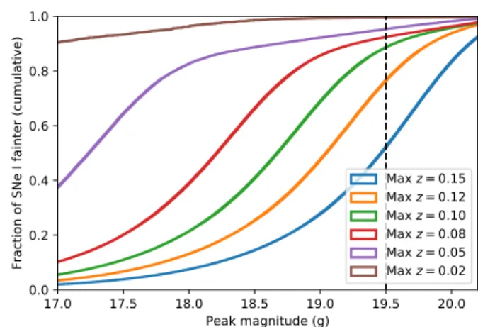
To make the published candidate stream even more pure, the following additional cuts are made prior to submission. First, we restrict the sample to transients brighter than 19.5 mag (the limit to which the channel content study was carried out). The magnitude depth will be increased once a sufficiently-low stel-lar contamination rate has been confirmed for fainter transients. Fig. 8 shows the expected cumulative distributions of peak mag-nitudes for SNe Ia below different redshift limits as determined by simsurvey. A 19.5 mag peak limit implies a ∼ 90% com-pleteness for SNe Ia at z < 0.08 based on the expected mag-nitude distribution. For the volumetric completeness this should be combined with the 80% coverage completeness determined above (which is mainly driven by sky position). We currently only submit candidates found above a galactic latitude of 14 de-grees to reduce contamination by stellar variables. An inspection of the so far reported candidates find less than 5% to be of likely stellar origin. Candidates compatible with known AGN/QSOs
17.0 17.5 18.0 18.5 19.0 19.5 20.0 Peak magnitude (g) 0.0 0.2 0.4 0.6 0.8 1.0
Fraction of SNe I fainter (cumulative)
Max z = 0.15 Max z = 0.12 Max z = 0.10 Max z = 0.08 Max z = 0.05 Max z = 0.02
Fig. 8. Cumulative simsurvey peak magnitude for simulated data, di-vided according to max redshift. Dashed lines show the current 19.5 depth of AMPEL TNS submissions.
are marked as such in the TNS comment field. TNS users look-ing for the purest SN stream can thus disregard any transients with this comment.
Two TNS bots are currently active: ZTF_AMPEL_NEW specif-ically aims to submit only young candidates with a significant non-detection available within 5 days prior to detection and no history of previous variability. This will create a bias against AGNs with repeated, isolated variability as well as transients with a long, slow rise-time but further rejects variable stars and provides a quick way to find follow-up targets. A second sender, ZTF_AMPEL_COMPLETE, only requires a non-detection within the previous 30 days.19
In summary, the live submission of AMPEL detections to the TNS provides a high quality feed for anyone looking for new, extragalactic transients brighter than 19.5 mag. The contamina-tion by variable stars is estimated at < 5%, the fraccontamina-tion of SNe to be > 50% and for SNe Ia with a peak brighter than ∼ 18.5 mag the SN Ia completeness is 80%, out of which ∼ 60% will be detected prior to ten days before lightcurve peak. Extrap-olating rates from the four (summer) month ZTF rerun would predict this program to submit ∼ 9000 astronomical transients to the TNS each year. The breaks due to typical Palomar winter weather makes this an upper limit.
7.2. Work towards an AMPEL testing and rerun environment The next AMPEL version is already being developed. We plan for this to contain an interface where users can directly upload chan-nel and unit configurations and have them process a stream of archived alerts. The container generation means that such a con-figuration could be automatically spun up in an automatic and secure mode at a computer center. This run environment would allow both more complete tests as well as more flexibility in car-rying out large scale reruns.
8. Conclusions
We here introduce AMPEL as a comprehensive tool for working with streams of astronomical data. More and more facilities pro-vide real-time data shaped into streams, which creates opportuni-ties to make new discoveries while emphasizing the challenge in
19 These bots replace the initial ZTF_AMPEL_MSIP sender, which is no