Applied Plasma Research

(1)

XVI. APPLIED PLASMA RESEARCH

A. Active Plasma Systems

Academic Research Staff Prof. L. D. Smullin Prof. A. Bers Prof. R. R. Parker

Graduate Students

N. J. Fisch G. H. Neilson A. L. Throop

C. F. F. Karney M. D. Simonutti D. C. Watson

J. L. Kulp M. S. Tekula P. R. Widing

RESEARCH OBJECTIVES

The research of the Active Plasma Systems group is concerned with the dynamics of highly ionized plasmas and charged-particle beams, with particular emphasis on under-standing and exploiting linear and nonlinear interactions in plasmas. In the coming year we shall add a new program of computer symbolic calculations of the nonlinear inter-action of waves in a plasma. Some of the major areas of research are listed below.

1. Wave Studies at Lower Hybrid Frequency

We are continuing experimental studies of wave phenomena near lower hybrid fre-quency. _{Our present emphasis is on the linear conversion of these modes at the} reso-nant point to warm-plasma ion sound modes that propagate across the magnetic field. The role of nonlinear absorption vs parametric instability is also being investigated. Our goal is to study the feasibility of lower hybrid RF heating of Tokamaks in a small-scale experiment.

R. R. Parker

2. Nonlinear Beam-Plasma Interactions

We have observed a nonlinear interaction between a modulated beam wave and an externally generated plasma wave, which leads to excitation of an ion-acoustic wave. During the coming year we plan to continue investigation of such nonlinear beam-related interactions in order to develop quantitative models of such interactions and determine their role in generating low-frequency spectra in beam-plasma systems.

R. R. Parker 3. Beam-Plasma Source

12 -3

A new plasma source has been developed which produces dense (10 cm ), hot

(10-20 eV), highly ionized (50%) plasma by extraction from dual beam-plasma sources into a differentially pumped drift region. We plan to make a thorough diagnostic survey

(2)

(XVI. APPLIED PLASMA RESEARCH)

of this plasma, with particular emphasis on the nature and cause of observed low-frequency turbulence. Attempts to stabilize the plasma are also anticipated.

L. D. Smullin, R. R. Parker

4. Computer Analytic Study of Nonlinear Wave Interactions

We are developing and using new computer capabilities in symbolic computation. At present we are applying this procedure to the problem of nonlinear wave interactions in a plasma. The coupling coefficients of all possible wave-wave interactions in a plasma can thus be derived and stored in analytic form by a computer. This will allow us to study the nonlinear parametric interactions of coherent waves, as well as the interaction of many waves for simulation of weak turbulence. This work will be carried out in cooperation with the Project MAC Mathlab, and will use the MACSYMA system.

A. Bers

1. OBSERVATION OF NONLINEAR INTERACTIONS IN A BEAM-PLASMA SYSTEM

NSF (Grant GK-28282X1) A. E. Throop, R. R. Parker

Introduction

In this report we shall discuss results of an experimental study of nonlinear wave interactions in a beam-plasma system. Detailed measurements of the waves partici-pating in the interaction have been made, and the results seem consistent with simple three-wave coupling-of-modes theory. Two specific cases will be discussed, both of which use a beam wave to excite lower frequency (LF) plasma modes. In the first case, an unstable ion acoustic spectrum interacts parametrically with a beam wave to excite an idler spectrum at the difference frequency and wave number. In the second case, two high-frequency (HIIF) waves interact to excite resonantly an acoustic wave. Only the qual-itative features of the interactions will be presented here.

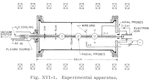
Experimental Apparatus

The experimental apparatus is shown schematically in Fig. XVI-1. At one end, a microwave structure produces a plasma column by electron-cyclotron resonance. This

10-3

plasma is fairly quiescent, with typical density of 5 X 1010 cm-3 and electron

temper-ature of 5 eV. At the opposite end of the experiment, an electron beam is injected into the plasma to excite the slow space-charge beam wave (SSCW). The electron source is an oxide-coated cathode that provides a beam with 2-keV energy and 15-mA current. The beam can also be modulated by applying a grid-cathode voltage. The diagnostics are Langmuir and RF probes, which can be scanned both axially and radially. Wire

(3)

(XVI. APPLIED PLASMA RESEARCH)

AXIAL PROBES

H 0 COOLING E E WIRE GRID 0-2kV

VACUUM GUN

SYSTEM

PLASMA SOURCEX

,- 66cm

-Fig. XVI-1.

Experimental apparatus.

grids (6 strands of

.

003 in. tungsten wire, crossed in wagon-wheel arrangement) are

used to launch and detect waves in the plasma.

These grids have been found to be

use-ful as a diagnostic for lower frequency waves (-100 kHz).

The experiment is operated

in a uniform 1-kG magnetic field, and typically uses argon gas at 6 X 10

- 5

Torr

pres-sure.

Beam Wave Characteristics

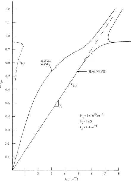
Since both interactions use the SSCW as a pump wave, it is important to understand

the properties of the beam wave. The basic model

2

_{in these experiments was the}

guided-wave dispersion relation (GWDR) shown in Fig. XVI-2.

The model assumed a cold

plasma and cold beam.

The addition of electron thermal effects does not substantially

affect the interaction. The GWDR was numerically evaluated for complex k I, assuming

real

o,

and left kI as a geometrically determined parameter.

Values consistent with

our experimental conditions were used to evaluate the dispersion relation. The GWDR

predicts that in the presence of the plasma the SSCW will be unstable over a broad

fre-quency band below the electron plasma frefre-quency (f pe).

Figure XVI-3a shows the RF spectrum obtained when the electron beam is injected

into the plasma column. As the beam current is increased, the spectrum increases in

amplitude and broadens to include lower frequencies.

The HF emission can be tuned by

varying plasma density (the microwave source power).

Langmuir probe measurements

also show that the plasma frequency is slightly above the HF emission, as predicted.

This confirms that the HF emission is due to the unstable SSCW.

The SSCW used here, however, is obviously not suitable as a pump for narrow-band

interactions, because of the lack of coherence and the broadband nature of the spectrum.

To obtain a more useful beam wave, we modulate the beam at a frequency within the

unstable SSCW region.

This entrains the energy into a narrow, well-defined beam wave

(4)

(XVI. APPLIED PLASMA RESEARCH) / BEAM WAVES N = 2x 1010cm- 3 B = 1kG kl= 2.4 cm-1 3 4 5 kll (cm- )

Fig. XVI-2. Guided-wave dispersion relation for cold beam and cold plasma.

at the modulating frequency, as shown in Fig. XVI-3b. Here we display a small por-tion of the broadband emission of Fig. XVI-3a, but on a greatly expanded frequency scale. The spectrum is centered at the modulating frequency and shows the emission with modulation on and off - all other beam and plasma parameters are unchanged. The bandwidth has been decreased by well over a factor of 1000, while the amplitude change caused by the entrainment is apparent from the photographs.

Figure XVI-4a shows a typical RF interferogram of the entrained beam wave. The wave grows, saturates, and decays over a large axial distance. The saturated region, over which the wave amplitude is quite uniform, is obviously an ideal position in which to study nonlinear interactions. The wavelength of the entrained beam wave can be

0.8 b,

(5)

BROADBAND BEAM-PLASMA INTERACTION I I I I I I I I 0 0.4 0.8 1.2 FREQUENCY (GHz) MODULATED BEAM

Fig. XVI-3.

(a)

RF spectrum of the unmodulated beam

injected into plasma.

(b) Detail of RF spectrum showing energy

entrainment. (Same vertical sensitivity

in both pictures.)

SUNMODULATED BEAM I I I I I I I I I I

S

-

I--300 KHz f= 1.2 GHz BEAM WAVE I I I I 0 5 10 15 20

AXIAL DISTANCE FROM GUN (cm)

(a) p 5x cm/s Vp=I. 5X10 9 cm/s I I I I I I I 0.1 0.2 0.3 0.4 0.5 0.6 k ~ _X(c m') Fig. XVI-4.

(a) RF interferogram of entrained slow

space-charge beam wave (SSCW).

(b) Measured beam wave dispersion relation.

0.7 0.8 0.9

0.6 [

0.4

_ ________ _~_

(6)

easily measured, and the dispersion relation shown in Fig. XVI-4b is obtained. The beam wave exhibits a phase velocity that corresponds to the gun voltage, and tends to show the expected dispersion as the modulating frequency approaches

ope

(see Fig. XVI-2). These measurements confirm that the modulated SSCW provides a coher-ent, well-defined wave that can be used as a pump to study nonlinear interactions in the plasma column.

Acoustic Wave Characteristics

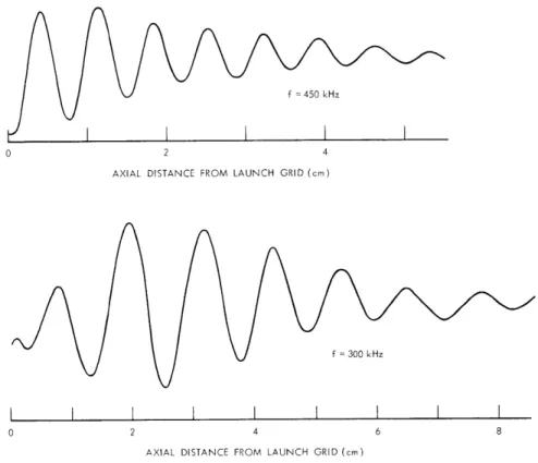
Since the expected nonlinear interactions involved coupling to an ion-acoustic wave, the propagation characteristics of these waves were studied in some detail. For these experiments, the waves were launched from the wire grid and an RF probe was used as

AXIAL DISTANCE FROM LAUNCH GRID (cm)

f = 300 kHz

I

0 2 4

AXIAL DISTANCE FROM

Fig. XVI-5.

I I

6

LAUNCH GRID (cm)

Examples of interferograms of ion-acoustic waves.

a receiving antenna. Over the 150 kHz-2 MHz frequency range, the wave (in argon) dis-played very light damping and, in some cases, even growth in the presence of the beam. Figure XVI-5 shows two examples of typical interferograms. Typical damping rates

-2

are in the (ki/kr)

=

10

2

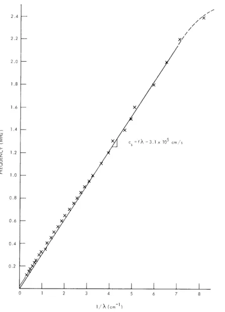
range. For frequencies above approximately 2 MHz, however, the waves become highly ion Landau-damped.

Figure XVI-6 shows the acoustic wave dispersion relation measured in the plasma

I

8

(7)

X

FX = 3.1 x 105 cm /S

2 3 4 5 6 7 8

1/X (cm- 1)

Fig. XVI-6.

Measured dispersion relation for ion-acoustic waves.

column without the presence of a beam. The phase velocity of the wave agrees well with the sound speed calculated for argon. The sound speed is not substantially changed by the presence of the beam. The dispersion that occurs at frequencies less than

800 kHz is not fully understood. The GWDR, however, exhibits a similar tendency when it is evaluated in the acoustic regime. In these calculations, the group velocity of the ion-acoustic branch slows considerably near w klcs. This suggests that for small values of k₁₁a finite kl could contribute to the magnitude of k, and hence cause the observed dispersion.

These data suggest that the lightly damped acoustic spectrum represents a strong fluctuation background. In the presence of free energy, either in the form of the

(8)

negative-energy SSCW or parametrically supplied energy, waves

can therefore be

expected to grow from this fluctuation background.

Parametric Interaction

Under certain beam and plasma conditions, it is possible to excite a

low-frequency

spectrum such as that shown in Fig. XVI-7a.

The spectrum typically extends over the

0. 1-2 MHz frequency range, which is the same frequency band

over which the acoustic

spectrum is lightly damped.

This and other data suggest that the spectrum grows from

I I I I I

0 1.0 2.0

FREQUENCY (MHz)

(a)

Fig. XVI-7.

(a) Low-frequency spectrum excited by electron beam.

(b) Sideband produced by the IF spectrum

parametri-cally interacting with beam wave.

2.0 10 0W

500 kHz tI.2 GHz

(b)

an unstable acoustic branch, although the specific details of the generation

of this

spec-trum are not of interest in this report.

If we now introduce an HF pump in the form of an entrained beam wave, the LF

spec-trum can interact parametrically with it to produce an

w- and k-matching idler wave.3

This is demonstrated by the HF spectrum shown in Fig. XVI-7b, which was

taken

simultaneously with Fig. XVI-7a.

The idler and LF spectra are mirror images of each

other, as expected, and have the same general profile.

The slightly smaller spectral

width of the idler spectrum is probably caused by threshold effects.

This interaction

(9)

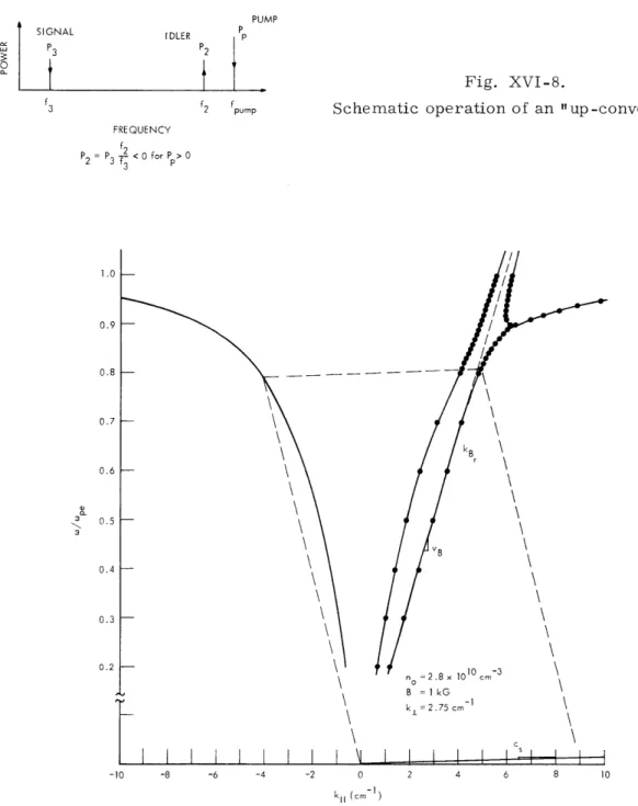
Fig. XVI-8.

Schematic operation of an "up-converter."

FREQUENCY P2 = P < 0 for P > 0 1.0 0.9 0.8 0.7 0.6 0.5 kB \ n =2.8 x 1010 cm- 3 B = kG k =2.75 cm-1 -10 -8 -6 -4 -2 0 2 kll (cm- )

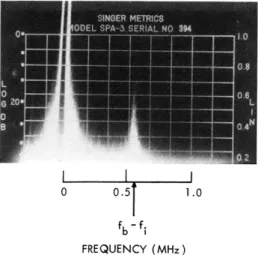
Fig. XVI-9.

GWDR showing a resonant interaction with the acoustic branch. (Acoustic branch not to scale.)

SIGNAL P₃

t

PUMP IDLER f2 pump 8 10

(10)

(XVI.

APPLIED PLASMA RESEARCH)

is identical with that which occurs in an up-converter, as shown schematically in Fig. XVI-8. A signal at f3 is parametrically amplified at a higher frequency f2 (idler)

with a gain of f2 /f 3. The energy is supplied by a pump wave at f = f₂_{+ f3'}

The pronounced peak in the low-frequency spectrum at -450 kHz might also be explained by a parametric interaction if we consider the GWDR shown in Fig. XVI-9. If we assume that the LF spectrum does correspond to the acoustic branch, then a k_res

res -1

is determined by k re

_res

s -

_c

= 9. 0 cm . Typically, wave numbers of the entrained

s-1

beam wave are in the range kb z 4-5 cm . Thus k-matching is possible only for a

coupling between the forward acoustic mode and the backward plasma wave, as shown in Fig. XVI-9. Because of the bandlimited nature of the LF spectrum, k is

essen-res

tially constant over a corresponding idler-wave spectrum. Therefore, only a single value of co exists which will couple resonantly with the acoustic branch. Other values of w will be driven off-resonance and thus give rise to the lower amplitude spectrum that is observed. The quantitative parameters predicted by this model, therefore, seem correct. Although the incoherent and broadband nature of the beam-excited LF spectrum makes standard interferometry difficult, we are attempting other techniques to identify the waves and processes involved. We wish to point out, however, that other beam-related processes may be responsible; for example, a change in equilibrium configu-ration or current-driven instability induced by the beam.

Mode -Coupled Interaction

To study mode-coupled interactions, two HF waves were excited in the plasma. One wave was the entrained beam wave which we have discussed. The second wave was

LOCAL OSCILLATOR INPUT

(11)

excited by applying several watts of RF power to a wire grid in the plasma. These two

waves can then be expected to drive a difference-frequency wave, even if it is not a

natural mode of the plasma. The interaction will be strongest, however, if the difference

w

and k do correspond to a natural plasma mode.

Figure XVI-10 is a schematic

dia-gram of this experiment.

Samples from the HF oscillators are mixed, and the

differ-ence frequency is used to measure the wavelength of the LF wave.

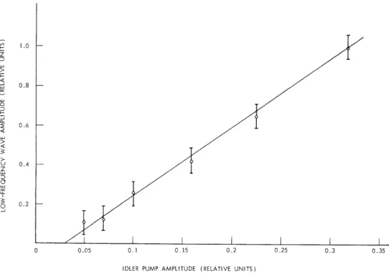
Figure XVI-11 is a spectrum analyzer display of the LF wave.

The frequency of

this wave corresponds to the frequency difference between the oscillators, and can be

Fig.

XVI-11.

Low-frequency spectrum showing wave excited

by two HF fields.

0 0.51 1.0

fb- f

FREQUENCY (MHz)

tuned accordingly.

Wavelength measurements were often complicated by the presence

of the beam-excited acoustic spectrum.

To prevent this, sufficient helium was added

to the vacuum chamber to Landau-damp the spectrum.

The nonlinear interaction,

how-ever, is strong enough to remain essentially unaffected by the small change in damping

rate. Simple three-wave coupling theory for two constant HF pumps predicts that the

excited wave amplitude should be proportional to the "idler'" wave amplitude. This is

confirmed experimentally as shown in Fig. XVI-12.

The result of an experimental dispersion analysis is shown in Fig. XVI-13.

The

wavelength of the LF wave is constant over the full range of the interaction. The wave

amplitude, however, shows a pronounced resonance at a frequency which corresponds

to a phase velocity equal to the sound speed in the plasma. While the LF wave is driven

off-resonance from the acoustic branch, the wave amplitude remains constant. When

the HF waves can interact resonantly with the acoustic branch, however, the wave

amplitude increases significantly and displays a very sharp resonance.

Additional data revealed that the wavelength of the entrained beam wave was equal

to that of the LF wave.

This implies that the wave number of the idler wave must be

zero.

This suggests that our wire grid is exciting an electrostatic field that has a

QPR No. 108

__

(12)

0.05 0.1 0.15 0.2 0.25 0.3 0.35

IDLER PUMP AMPLITUDE (RELATIVE UNITS)

Fig. XVI-12. _{Amplitude of difference-frequency wave vs amplitude of pump field.}

4.5 4.0 3.5 3.0 S2.5 _ < 2.0 J 1.5 rr 1.0 1.6 E o 1.4 (D z 1.2 J Uj 200 300 400 500 600 FREQUENCY (kHz)

Fig. XVI-13. Amplitude and wavelength dependence difference of HF fields.

(13)

(XVI. APPLIED PLASMA RESEARCH)

resonant cone structure.4, 5 Such a field exists only along a specific angle to the mag-netic field. At all points along this angle, the field is in phase and exhibits essentially infinite wavelength. It is not really surprising that our grid excites this type of field,

since the geometry is very similar to that used by Simonutti, Parker, and Briggs.5 This explanation is also supported by the lack of any detectable wavelength associated with the idler wave, and the fact that the interaction strength is a function of radial position

and extends over a sharply defined axial length.

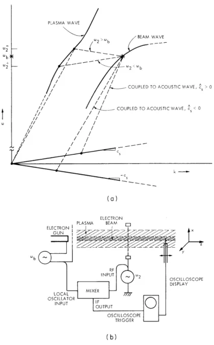
OSCILLOSCOPE DISPLAY

(b)

Fig. XVI-14. (a) Possible interactions with acoustic wave for cs > 0 and cs < 0.

(b) Experiment for measuring direction of wave propagation.

-e 5

(14)

(XVI. APPLIED PLASMA RESEARCH)

The magnitude of the two HF fields is approximately equal during this mode-coupled

interaction. We can therefore expect the LF wave to be excited if the frequencies of the

HF waves are exchanged.

Of course, the specific characteristics of the interaction may

change.

Figure XVI-14a demonstrates this schematically. Here a beam wave and

gen-eral plasma mode (or dipole field) have resonantly coupled with the acoustic branch.

The diagram indicates how the two waves could interact with either of the oppositely

directed acoustic waves.

This effect has been observed experimentally, as shown in

Fig. XVI-14b.

The frequency difference between the oscillators is used as a reference

Fig. XVI-15.

Low-frequency parametric interaction driven by

another mode -coupled interaction.

o

10oo kHz

SIGNAL

PUMP

IDLER

to measure the direction of phase shift of the LF wave as the receiving probe is moved

axially. We find, in agreement with our predictions, that

A A

c

s

= vb

for w2 < wb

A A

c

s

= -vb

for

2o

>

wb'

Finally, we offer Fig. XVI-15 as evidence of the strength of the observed

mode-coupled interaction. Again, two HF waves were used to excite an LF wave at 600 kHz.

In this case, however, the excited wave is sufficiently strong so that the difference

wave parametrically itself excites another lower frequency wave (perhaps a drift wave)

at ~100 kHz, as well as an energy-matching idler sideband. Although this photograph

is not typical, it is perhaps the best evidence that the excited LF wave is indeed a

strong, coherent, and well-defined plasma wave.

We acknowledge the contribution of Professor R. J. Taylor who suggested the

con-taminant Landau damping and P. Widing, whose computer code was used in the

numer-ical evaluation of the GWPR.

(15)

References

1i. A. Y. Wong et al.,

in IAEA/CN-28, Proc. Fourth Conference on Plasma Physics

and Controlled Nuclear Fusion Research, International Atomic Energy Agency,

Uni-versity of Wisconsin, Madison, Wisconsin, June 17-23, 1971.

2. _{R. J. Briggs, Electron-Stream Interaction with Plasma (The M. I. T. Press,}

Cambridge, Mass., 1964).

3. A. Bers, M. I. T. Course 6. 58 Notes, Fall 1971 (unpublished).

4. R. Fisher and R. Gould, Phys. Fluids 14, 857-867 (1971).

5. M. Simonutti, R. R. Parker, and R. J. Briggs, Quarterly Progress Report No. 104,

Research Laboratory of Electronics, M. I. T., January 15, 1972, pp. 196-201.

2. ANALYTIC STUDIES OF NONLINEAR PLASMA PROBLEMS BY

SYMBOLIC MANIPULATION PROGRAMS ON A COMPUTER

NSF (Grant GK-28282X1)

A. Bers, J. L. Kulp, D. C. Watson

Introduction

The simulation of charged-particle dynamics on a computer has greatly increased

our understanding of strongly nonlinear (in particular, nonlaminar) phenomena in

plas-mas. Such simulations are impractical for studying nonlinear phenomena whose time

and space scale of evolution is many orders of magnitude larger than the individual

par-ticle dynamics scales. Examples of such phenomena are the weakly nonlinear (either

coherent or turbulent) wave interactions in a plasma, and most of the phenomena

asso-ciated with the nonlinear (but laminar) fluid dynamics behavior of plasmas such as occur

in studies of transport properties and equilibrium configurations.

In contrast to

par-ticle simulations which require a large number of numerical computations, weakly

nonlinear phenomena can best be studied by perturbation techniques that require a large

number of symbolic computations.

Recent advances in the development of symbolic

manipulation programs now make it possible to build up and implement on a computer

analytic techniques suitable for solving nonlinear dynamics problems.

During the past year, in cooperation with the MATHLAB Group of M. I. T.'s Project

MAC, we have initiated such an implementation. Our first focus is a study of the

non-linear wave interactions in the fluid model of a plasma in a magnetic field. All of the

work is being carried out on the Project MAC Symbol Manipulating system called

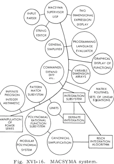
MACSYMA (see Fig. XVI-16). This is a hierarchical, evolving computer system with

specific capabilities for symbolic manipulation of algebraic expressions and

mathemat-ical operations.

A detailed description of this system appears in the "Proceedings of

the Second Symposium on Symbolic and Algebraic Manipulation" (March 1971).1 These

(16)

Fig. XVI-16. MACSYMA system.

proceedings also provide a useful overview of this computer field.

In this first report we present a brief description with illustrations of various ana-lytical capabilities of MACSYMA, and show the use of this system in the study of non-linear wave interactions in plasmas.

General Description of MACSYMA

MACSYMA is a symbol-manipulation system in which various mathematical opera-tions can be carried out in analytic form. A symbolic manipulation system is one in which inputs are expressions or equations in symbolic form. Mathematical operations are carried out on these expressions, and answers are returned in a two-dimensional display of symbolic mathematical form. This system is useful for obtaining analytic solutions to problems, as opposed to the conventional numerical analysis for which com-puters have been more commonly employed. The ability to interact with a derivation and control its progress is very important. Thus the basic mode of operations of MACSYMA is conversational; it is implemented on a time-sharing computer system (DEC-PDP 10).

(17)

Many of the interesting capabilites are briefly discussed in this report, with simple examples given which are intended to illustrate the meaning of features rather than their power in handling realistic problems.

a. Expression Manipulation

This type of command includes strictly algebraic operations encountered in symbolic manipulations. _{Examples of expression manipulation are shown in Fig. XVI-17.}

1. Simplification. _{Finding expressions which reduce to zero or one; canceling} com-mon factors; simplifying special cases as in trigonometric functions, noncommutative multiplication, matrices, and calculus operators.

2. Expanding expressions.

3. _{Extracting parts of an expression; taking coefficients; taking real and imaginary} parts.

4. _{Substitution; substituting for extracted parts.}

5. _{Factoring over the fields of integers, Gaussian integers (integers X -i),} _and some algebraic numbers.

6. _{Polynomial manipulation; raising to a power; division; partial fraction and} continued-fraction expansions.

b. Evaluation

Evaluation can be either numerical or symbolic. An example of symbolic evalua-tion is the following. Let A be assigned the value B+C. This is A:B+C in MACSYMA notation. _{If we then input EVALUATE (A ), we get (B+C)}2 _. _{Numerical evaluation is}

illustrated by the following. _{A:u/4, EVALUATE (sin A, NUMER); the return is 1/2.} This capability is important because once an expression is derived symbolically, there is no need to write a computer program to evaluate it numerically. The expression is, in a sense, already programmed in the system.

c. Matrix Manipulation

All standard vector-matrix operations are available: transpose, inverse, matrix multiplication, determinant, characteristic polynomial, extraction of a coefficient matrix from a set of equations, differentiation, integration, and any other operation that can be applied to an ordinary scalar expression. Examples of matrix manipulation are shown in Fig. XVI-18. Extensive array and list structure capability is included.

d. Calculus

Most standard calculus operations are available. Examples of calculus operations are shown in Fig. XVI-19.

(18)

Explanation: The Ci lines are commands or expressions typed by the user,

while the Di lines are the computer responses. "0" terminates a cormand.

"B" stands for the last expression mentioned (i.e. the last Ci or ri line). The " " character indicates that a function or command is to be displayed

but not evaluated or carried out. Also the command EXP,EXIAND is

equiv-alent to EXAND(EXPR). RATSIMP is a command which tries to put expressions in a ratio-of-polynomials form and also doer simplification.

SIMPLIFICATION EXAMPLE:

Note that simplification is automatically invoked at the end of any operation.

(Ci) A + (X*E+B*(A/F-X)) 0 A E (- - X) + F X + A (D1) (C2) RATSITP(D1)' (D2) 2 A

Here, the simplifier has noticed that -EX + EX is ecuivalent to 0 and A+A is 2A.

EXPANSION EXAMPLE:

The FXPAED command carries out distribution of onerators such as multiplication

(and some linear and bilinear operators), as well as, matrix multiplications.

Many options are available to control the extent of expansion.

(Cl) EXPAND((A+F)**4)G (D11) 4 3 2 2 S+ 4 + 6 E +4 A B+A (C2) EXPAITD((X+Y)**2*(A+E)*2)C 2 2 2 2 2 2 2 (D2) B Y +A A Y2A Y 2 X Y + 4 A X Y + 2 A X Y 2 2 2 2 2 +B X + 2 AE X +A

Now consider an example of rationally simplifying and factoring expanded expressions.

(cs) D1/D20 4 3 22 3 4 (D3) (B + 4 A E + 6 A B + 4 A E + ) 2 2 2 2 2 2 2 2 2 /(E Y + 2 A B Y + A Y + 2 B X Y + 4 AB Y + 2 A X Y + B X 2 22 +2ABX + X) (C4) FACTOR(RATSLP(D3))@ (B + A) (D4) 2 (Y + X)

PATSIMP has canceled out the factor (A+B)**2 which is not easily seen in D3. An example of expanding the integrate operator.

(C5) 'INTEGPRATF(A*F(X)+E*G(Y) ,X,N,,INTF) INF (D5) (L G(X) + A F(X)) DX (C6) DECLARE( INTEGRATE,LINEAR)$ (c7) D5,EXPANDO (D7) INF E (I G(X) DX) MIN INF + A (I F(X) Dx) MIN

(19)

E'TEACTIOI OF PARTS EXAIPLE:

To extract the 4 th term in the denominator of 13, first "circle" it to see if that is the term we want, an( then extract it.

(CE) 7PART(37,2,4)X

4 3 22 4

(PE) ( +4 A E +6A +4A + A )

22 2 2 2 * 2 /(E Y + 2 A B Y + A Y + *2 XY* + 4 A B X Y + 2 X Y 2 2 2 2 2 + E X + 2 A B X + A X ) (Co) PART(D,2,A)) (D9) 2 P X Y

To extract rational coefficients, sRATCOEF is used. Here the coefficient of A**4 in (A+E)**8 is found.

(C11) ?ATCOE((A+B)**"8,PA**4)

(D11) 70 E

(C12) (X+A)*(Y+3)**2-(X+A)*COS(A)*-2-(Y+C)**7=

(D12) - (Y + C) 3 + (X + A) (Y + 3) 2 - COS (A) 2 (X + A) = C

S2 2 2 2

(D1I) -Y +XY -3CY +AY +6XY-3C C Y + 6 A Y - COS 2(A) X+ 9 )-C

2

- A COS (A) + = O (C14) P TCOEF(LS(<),X+A)

2 2

Y + 6 Y - COS (A) + 9

Note the the left-hand-side operator had to be used, since equations are not rational expressions. The coefficient of X+A is not evident in D13. The use of HATCOEF and RATS3UST (below) makes it possible to control the size and form of expressions.

Taking real and imacinary parts is illustrated below. natural logs, and II is the sqrt(-1)

(c015) E-H(I*AGLF2) (D15) (1Cm6

REALPART(3')@

(c17) (A+I*B)/(D+jI*E)C (D17) (C1i) IA!,GPAT()@ (Cl) RATSIDP(D1O)C C"I ANICLE COS(AINGLT) L

E is the base of the

'I E + A I E + D EDL 2 2 E + D AE 2 2 E +D AE-BD 2 2 + D

Fig. XVI-17. (continued) (D104)

(20)

SUBSTITLUTIOI FXAMPLES:

The substitution for extracted parts is illustrated.

First, consider substituting W[PE]**2*F[O] for Q**2*0O/ . (C1) Q*2*lO*E/M/EI/W@ (D1)

7I

E NO QC M U-(C2) RA.TSUST("[CE]**2*EP[C],Q*2*iC/i, ) 2 TI FP E 0 PE (D2)

--(cs) (X+A)*( Y+) **2-(X+-)*COS(A )**2- (Y+C)

**=-2 2 (rs) - (Y + C) + ( + A) (Y + 3) - COS (A) (:, + A) = O (c4) DFA i( ) 2 2 2 2 (D4) - Y + X Y - 3 C Y + A Y + 6 Y- 3 C + 2 A Y - COS (A) X + 9 X - C 2 - A cos (A) + 9 = 0

In this exarple .ATSUEST must effectively extract the factor X+P and

then substitute XEAC for it.

(c5) RATESUBST (XAC,X +A, LS (14))

(Ds) - Y + (XPAC -3 3 C) Y + (6 2 XIAC - 3 C ) Y 2 - COS (A) XPAC + 9 X'FAC - C The

RAT

command reorders the expresion with XFAC as the most important variable. (C6) RAIT(l,XAC)!

2 2 3 2 2 3

(D6) (Y + 6 Y - COS (A) + C) ?AC - Y -

3

C Y - 3 C Y - C

It should be noted that RATSUST soretimes has strange effects when substituting

for a simple factor such as Y+C.

FACTORICG 7DAVIPLE:

An interesting factoring problem.

(CI) X**9G+ X +1 (D1) (C2) FACTOR(, ) 2 6 10 9 7 6 5 4 (D2) (X + 1) (X - X + 1) (IX - X + 1) (X - + + - X -X + X - X + 2 - X 20 19 17 16 14 13 11 10

5

7 6 4 + 1) (X +X -X - + + -X - - + +X -X - + X + 1) 60 57 51 48 42 79 ER 30 27 21 1c 12 9 3 (X + X -X -X + X + - - - X + X +X -X - X + X + 1)

(21)

PARTIAL FRACTIOR EXPANSION EXAMPLE: (Cl) (X+2)/(X+3)/(X+B)/(X+C)**2C X+2 (D1) 2 (X +

5)

(X + F) (X + C)

This shows the main use of RATSIMP - to put expressions in ratio-of-polynomials form. The most important variable is assumed to be X.

(C2) RATSII(5)C.

4 3 2 2

(D2) (X + 2)/(X + (2 C + E + 3) X + (C + (2 B + 6) C + 3 E) x

2 2

+ ((B + 3) C + 6 B C) X + 3 C)

Now take a partial fraction expansion of this ratsimped expression. The answer would be the same as if we had expanded D1 directly, but it is less obvious from this form.

(C3) PAF FPRAC(,X)C 2 2 (D3) - ((C - 4 C - B + 6) X + 2 C + ( - B - 9) C + (4 E + 12) C - 6 B) 4 3 2 2 2 2 2 /((C +(- 2 B- 6) C + (B + 12 E +

9)

C + ( - 6 B - 18 E) C + 9 E ) X 5 4 2 3 2 2 2 + (2 C + ( - 4 B - 12) C + (2 EB + 24 B + 18) C + ( - 12 B - 36 E) C + 1E B C) X 6 5 2 4 2 3 22 + C + ( - 2 E- 6) C + (B + 12 B+ 9) C + ( - 6 B - 18E) C + 9 B C) 2 2 3 2 2 2 + (B- 2)/(((E - 3) C + (6 B - 2 ) C + B - 3 ) X + (E - 3 F) C 2 3 3 + (6 - 2 B ) C + B - 3 B ) 2 2 - 1/(((B - 3) C + (18- 6 E) C + 9 E - 27) X + (3 E - 9) C + (54 - 13 B) C + 27 B - 81)

This does not look like a martial fraction expansion because factors have been

multiplied out. To see this we use a function we have vTitten in MACSYIA which

factors terms in a sum and subexpressions. It can now be seen that the factors have been expanded above.

(C4) FACTERMS(%)@ B-2 1 (D4) 2 2 (E - ) (C - B) (X + ) (E- 3) (C- 3) (X + 7) 2 2 (C - 4 C- B + 6) X + 2 C + ( - -

9)

C + 4 (E + 3) C- 6 P 2 2 2 (C - 3) (C - B) (X + C)

Now we refactor to obtain the original result. (C5) FACTOR(%)@

X+2 (D5)

2 (X+ +(X

3

+ E) (X + C)

SUMgARY: It is important to notice how these commands can

be

used to reduce the

complexity of exoressions and for restructuring them in a desirable form. Also, as in the factorlng case, simplifying procedures can lead to unwanted results

which are larger than what was started with. By interactin with expressions,

these problems can be avoided.

(22)

FAISPLFS OF iiATRIX CPFATIONS:

The first example is taking the inverse of a matrix which occurs in the cold plasma theory (resultinr in the mobility tensor). ( )**(-1) is taking the inverse of 01. " means o "assiFgi to".

(C1) II;VFSLiOPC (C2) AT:EV(( )**(-1),ATSI2po ) (C2) *W .I - WC 0 * * C 0W II 0 * * O O :', ,I* * ; -_T : * 2 2 * WC - iW WC 2 2 2 2 WC - .

The ALIA3 comrand is used for atreviatin, long races. (C) IAS(CC, COC:PLLe(COJ, ', TFL 7 !)o

relow several rmatrix onerations are illustrated including multiplication and differentiation. The example is the calculation of the time averaged energy in the linear modes of e cold plasna. 1. is frequency, 2P[C] is the free space

ieiectric constant. "*" as a superrcript indicates complexconjugate. cte that the an:wer is in an awkwsrd form. rhis is a eneral problen of symoolic manipultion systens.

(C4) -PIL(o) :=-P[O]*IDEZT(3) + F***- 'i[O]*";AT/ I/

2 * 0 .0T .1 (N ) EPSILO(I.) := E 11 0 * 2 2 2 * -0 Ti -' * 2 22 I* 0 0 -- * W * (C5) CC(TT( )). r z(EoSIT (,), ). 1/4 * f--I ' * 2 2 * WC - W 2 * WC

LI

kPE 0 *- _ 0 * 2 2 * WC -* * * ** *E E F * *X V Z* *1 0 F * ((- (Io *o 1 to i 0 0 (rP) (C6) FACTOE( V(C,Dr m,D AIr)) 2 4 2 (r6) (E1P -E (! (2 *V * + 2 * * 0* Z* * Y* 2 +2 * ) * Z* 4 2 + 2 WC *E * * Z* 2 2 2 4 W WC *E * * Z* + "I W WC (3 F - - F Y ) + :I \ WC (E F E - E ))) - / Y X Y 2 2 /(2 W (wC + W) (C - w) )

Fig. XVI-18. Examples of matrix operations. 0 * C * I* -.,C 2 2 !C -I 2 2 2 WC - , O * 0 * ' I* *E S* * * -)) . *E *)_{• y*}

(23)

DAIPLES OF CALCULUS OPERATIONS:

Below are examples of the DIFF command which carries out differentiations. (cl) X^2*SIN(X)+Y*X+%F**(X^2)/X+COSI (X)<G

X Y + X SIN(X) + COSE(X) +

-(C2) DIFF(D1,X)6

2 fF

Y + 2 X SIN(X) + X COS(X) + SINH(X) - -- + 2 E

2

X

The period operator "." is noncommutative multiplication which can matrix multiplication or for definin, operators such as "GRID." . must depend on t.

(C7) A.E+C.DC

te used for vector or iote that A,F,C,P

C. D+ A .

(C4) DIFF(D,T)C

DC PD DA DB

- . D + C . - + - . + A .

--DT DT DT DT

Here the special gradient definition feature is shown. defined as r'(x). (C5) (C6)

(D6)

The derivative of F(x) is

GRADEF(G(X),?G'?(X))O

'DIFF(G-(X),X) = DIFF(G(X),X)C G(X) = G'(,)

Fig. XVI-19. Examples of integration in MACSYMA. (D1)

(P2)

(Ds)

(24)

An example of indefinite real domain integration with verification of results. (C7) INTEGRATE(1/(X**3+A**3),X) [ 1 I DX /X +A (CE) EV(,,INTEGRATE) 2X-A 2 2 ATA( --- ) LOG(X - AX + A ) SQRT(3) A LOG(X + A) - + + 2 2 2 6 A SQRT(3) A 3 A (Ce) DIFF(7,X,1) 2 2X-A 2 2 2 2 S(2 X - A) 6 A (X - A X + A ) 3 A (--- + 1) 2 2 3 A (X + A) (C10) RATSIIMP() (D10) 3 3 X + A

Consider a complex contour interral that occurs in plasma problems.

51(W,

x)

(D1) /F Q E(W., x) (I ] 1IN1 5KI (-- _PVF (V))₀ ( - --- ) DV) W- K V

Evaluate this integral for fO(v) a Lorentian distribution. Note w must have an imaninary

part since the integration command drops the imaginary part of real integrals.

(C2) ,[)(V)=./RPI/(V^2+A^2), ' -= + I*W:/I , I FC S+

)

(I Ci F-(',Z +r Y1' U:, x) (}F 11(WR +

GI

WI, K) 2 7I AV ] 2 / 7P1 (V KiI1T 22 +A

)

('R + iI WI - x V) NO i

(C3) T,T=EV(, ITEGRATE), WR=W, WI=O0

(3) (, K) ;I K Q E(,, K)

O0 2

S(5 w + K)

Fig. XVI-19. (continued)

(D7) (DE) (Ds) (D2)

_II_

- ---

(25)

~----(XVI. APPLIED PLASMA RESEARCH)

Special operators such as GRAD, DIV, CURL can be implemented.

2. Integration - indefinite integrals, definite integrals, complex contour integrals (residues), including some branch cut integrations. Integrals are actually worked out as opposed to being looked up in tables.'

e. Solution of Equations

Capabilities available on MACSYMA are listed here; other techniques for special problems can be adapted from these.

1. Solution of systems of linear algebraic equations.

2. Solution (or at least partial elimination) of sets of nonlinear algebraic equations. 3. Ordinary differential equations (also Laplace transforms).

4. Solution of differential equations by power series methods. 5. Solution of linear vector-matrix equations.

6. Solution of some integral equations.

Examples of some of these are shown in Fig. XVI-20.

f. Summation, Indexed Products, Limits, Power Series

Infinite or indefinite sums or products can be evaluated or manipulated. A powerful power series package is being implemented but has not yet been debugged. Taylor,

Laurant, and user-written functional power series expansions are available. Examples are given in Fig. XVI-21.

g. Pattern Matching

This feature allows a user to build new information into the system; vector identi-ties, trigonometric identiidenti-ties, special functions (Bessel, Zeta - the plasma dispersion function, etc.), operators, and other useful conventions can be handled in this way.

h. Auxiliary Features

System control commands, disk-file storage, string manipulation, programming, editing, plotting, graphing, input-output commands, aliases (abbreviations), debugging, association of names and properties, and display are included.

In addition to the features mentioned, MACSYMA "knows about" complex variable algebra, trigonometric, hyperbolic, and exponential functions (including Arc functions), special values such as

Tr,

e, -, Bernoulli and Euler numbers. Also MACSYMA can do numerical calculations to any desired degree of accuracy (with a price paid in speed).

Most of these features of MACSYMA are needed when the solution to a realistic prob-lem is attempted, and the fact that it has so many sophisticated capabilities encourages us about the prospect of overcoming difficulties encountered with other algebraic manip-ulation systems. These difficulties arise, for the most part, because of the inability of

(26)

SOLUTIOI OF EQUATIONS EXAMPLES:

The solution of a set of 3 by 3 linear alreraic equations.

(C2) A*X+ *Y+C*Z25: (D2) C Z + E Y + A X = 25 (C') 2*X+4*I+8*Z=1w (D7) -Z + 4 Y + 2 X = 1 (C4) X+Z=o (D4) Z + X (Cs) SOLVE( [D2,D3,D ],[X,Y,S]) SOLUTION 4 - 10o (:5) = 4C-6B-4A c - A- 150 (E6) Y =---4C-6E-4A E - 100 (27) Z = -4C-6E-4A (D7) [, 6, E7]

Eelcw is an example of solvin nonlinear al,-ebraic equations. Several techniques are used but tically the set of ecuations is rut in a polynomial for where the main

variables in the polynonial are functions of the variables bein_r solved. Then

poly-rnoial

solving

techaiques are used, and functior inverted. Also, sets of ecuations

are solved ty elimination.

(C"f) - 12*X +S:X**2 +

S,

(CS) SI (XS)**2-5*I;;(s)+30 22 2 (D) SII (X - 12 X + 1) - 5 SIN()( - 12 2' + =) + 3 (C10) SOLVS( ,X) SOLUTIOi (E10) X = 6 - SqCT(A3IE( - -T1 ) + 3) 2 SQR(1) - 5 (El) -X : ST(A;I;L( - --- ) + 3-) + i 2 SCRT(13) + 5 (E12) X = 6 - SQ:T(AI(--- ) + 3) 2 ( )3(LT(13) + 5 (E17) I : = -,c:;(ACTX;( -) + 3) + 5 (D14.) [ I, 11, 12, '3]

This is an examnle of the solution of a first order ordinar.- differential

equation (-ernoulli equation). COSI is an interation constant. (C15) X*2*(X-1)*'IrFF(Y,:) + Y**2 -X*(:-2)*YT

2 Fly 2 (D15) (X - 1) - + Y - (X - 2) Y (C16) SCLPIF-11(/) (DIE) CoST - + -(2 - 1) Y X - 1 (c17) SOLVE(,;,Y)G 2 (D17) I =

Fig. XVI . Examples- ) -solution of equations on

(27)

FXAMPLES OF TAYLOR SERIES AND LIMITS:

Althourgh there is a built in Taylor series command, consider, as an example of proramming in MACSYMA, a function written in the MACSYMA language which computes Taylor series.

TAYLOR(EXPR VAR,POINT, HIPOTR):=

BLOCK ( [RESULT],C ESULT: SUEST(POINT,VAR,FXP-R), FOR I:1 THRU HIPOWER

DO [EXPR: DIFF(EXPR,VAR) / I,

RESULT: RESULT + (VAR - POIIT)^I * SUBST(POINT,VAR,FXPR)],

RETURN(EESULT) )

As a simple example of Taylor series expansions, consider the expansion of SIN(X)/X

in X about XO to third order.

(CI) TAYLOR(SIN(X)/X,X,NO,3)9 2 SIN(XO) 2 SINI(XO) (X - X0) (- + XO

(D1)

2 COS(XO) - ---- ) 2 XO 3 3 SIN(XO) 6 SIN(XO) (X - XO) (--- - ---2 4 XO XO COS(xo) 6 COS(XO) X0 _XO3

cos(:0)

SIL(o)

si(XO)

(

) +

----XO 2 XO

XO

Consider the evaluation of this expression for XO =, PI/2 where ,PI is pi.

(C2)

6,XO-PI/20

56 12 ( - ---- + -) (X 4 2 1 1pi ( P PI 3 16 -) (--2

_$PI

3 2 :I 2 ) ( - -) PI1 2 +

Now consider taking the infinite magiietic field limit of the mobility tensor for

a cold plasma. This is done by taking the limit as WC :oes to infinity.

( C3) 'LIIT(SAT, WC, INF) (;s) (04) Fig. XVI-21. GI v 2 2 * WC - W * WC LIMIT * --11C ->INF * 2 * WC -* 0

Example of series expansions and limits.

WC 2 2 WC - W 2 2 WC - W 0 * S* O * *c *I 0 - -* W. * + (X - XO) (D2) 'PI 4 (X -- ) 2 2 + -PI 2 1PI *0 0 0* *0 0 0* *0 0 -- * (C4)

9,LIMIT

(28)

controlling the size and form of expressions resulting from a derivation. While this is still a problem, MACSYMA has given the user several representations for expressions and some powerful commands for controlling the evolution of an expression through a calculation. Furthermore, advanced simplification and factoring techniques aid in reducing the size of expressions. The features and capabilities of MACSYMA have been described in greater detail elsewhere.1, 2

Use of the MACSYMA System in the Analysis of Nonlinear Wave Interactions in Plasmas

The initial problem that we are solving on MACSYMA is the derivation and evalua-tion of coupling coefficients describing the nonlinear coherent three-wave interacevalua-tions in a plasma.3 This coupling can be formulated as arising from the nonlinear current, which is given to second order in the electric field amplitude by

ab a b

(1)

zi= Oijk j k'

-a -b

where the summation convention is used, and E , E are the electric fields of all pos-=ab

sible linear modes (indicated by superscripts), and c is a third-rank tensor embodying the second-order nonlinear properties of the plasma. Once an expression for this cur-rent is found, evaluation of the coupling coefficients of the linear modes is straightfor-ward. The coupling coefficient for the linear modeZ is proportional to

- n - nab n* a

b

2 ijk i j k

Since we are primarily interested in the perburbation of the complex amplitudes of the nab nab n* a b

linear modes, we consider the quantity M =ijk e ej ek with e representing unit vectors (polarization) associated with the linear modes. We are exploring the use of

nab

MACSYMA in the derivation and then evaluation of M n a b These two steps are rather distinct and will be discussed individually.

a. Derivation of J

As a specific example to illustrate the general method, consider the derivation of J2 for a warm fluid plasma model. Note that it is sufficient to consider a single species because nonlinear conductivities for different species can be simply summed. To start, we type the following set of equations into MACSYMA:

(29)

(XVI. APPLIED PLASMA RESEARCH) Continuity: Equation of state: Faraday's law: an --5- + V - (nv) = 0 P= P n "Y 8B VX E = at"

Also, the relation J = qnV is needed.

In order to arrive at a simple physical interpretation to a particular nonlinear wave interaction, we would like to be able to identify the terms in the fluid equations which give rise to the coupling. _{If the force equation is divided by n, it is evident that the} following nonlinear terms occur in these equations.

1. (V) v

2. VXB

3. (Vn)/n 4. nv 5. Vnv

convective nonlinearity

Lorentz nonlinearity

pressure nonlinearity

current nonlinearity

continuity nonlinearity

The derivation of Eq. 2 is then set up so that the effect of each nonlinearity can be iden-tified in the final answer.

Once the equations are entered, a functional Taylor series expansion is taken of the equations in the variables V(r, t), n(r, t), P(r, t), E(r, t), and B(r, t) about an equilib-rium which we take to be homogeneous (n , P , B constant and V 0 0, E = 0). In prac-tice P might be eliminated first to reduce the number of variables, but this is not necessary. _{For the fluid model, the only nonalgebraic nonlinearity occurs in the} pres-sure term of the force equation, so it is sufficient just to expand this equation in n(F, t). The pressure term then to second order becomes

7 P 0 Vn yP y(y-1)Po

n

Y

n ₂ V(n-no)- 3

n

2n

2 YPo

V (n-no) + 3 (n-no) V(n-no). n

If we let P = n KT, then

VP Vn (n-no) Vn

= -yKT _n_n Y (y-2) KT _n _n (8

(30)

might be the amplitude of the electric field. --

~2--v(r, t) = v + L 1 (r, t) + L v2(r, t) ... (9)

n(, t) = no + Ln (r, t) + L n₂

(r,

t) ... (10)

etc.

The resulting equations are then ordered in powers of L and structured so that products of lower order terms are "driving" the higher order terms. These two steps of expanding and ordering are carried out by a single function that we have implemented, EXPEQS, which would then return

First-order equations: 8v₁ Vn ₁ m a -cTy + qE + qv X B (11)

at

n

1

0 O

an

1

+ n+nV

0 (12)

at o 1

aB

11 VX E (13) 1 _noVl"_nol ₍₁₄₎ Second-order equations:

8v

7n KTnl

Vn

I m n XB -m(v1 1( ) 2 + q I X B1 (15) o n 0 an

-n

V

-

₍₁₆

J2 = noV2 + nlv1. (17) 2

For three-wave coupling it is sufficient to carry this ordering to L , but for higher order interactions the procedure is continued to higher powers of L. This simply involves specifying to EXPEQS the highest power of L to be considered.

Now the equations are transformed by heuristic pattern rules such as - jw, S- -jk. Second and higher order equations containing terms like (.V)1 ) 1 are

trans-formed to convolutions in c and k space. If we assume that only a discrete set of first-order modes exists, then the convolutions are just summations. A single "trans-form function" has been implemented to take care of these continued operations. As an example, we show the result for the second-order force equation of mode n:

(31)

n

n -n +n 2 -n -- 1 -b b .a a -inmv + ikyK T - qv X B 2 - m(v kbv I + im v a 0 o a,b ab -b -b -a -a nlnl a -a 1 -b 1 iy(y-2)

KT

2)qv(+ 1 X b qv 1 X a

I'

(18) n Co 0

where cn a +C k = a b, and

B

1 has been eliminated by use of Eq. 13.

The next step is to solve the first-order (linear) equations for V1(0, k) in terms of E1 (C, k). This can be done by factoring the matrix operators relating all the variables,

eliminating nI, and then explicitly substituting vectors for Bo' V1' and El and directly

solving the vector equation. From this the linear conductivity can easily be found. At this point the linear dispersion relation can be derived directly. MACSYMA can then immediately evaluate this dispersion relation numerically for cases of interest or give C-k plots for a given set of plasma parameters.

The second-order equations are solved by noting that the left-hand side operator is the same as that for the linear case (this is also true for higher order equations) which has already been obtained. Finding J 2 is then a matter of solving for V2 by inverting the

left-hand side operator of Eq. 18 and writing n1v1 in terms only of products of E1. The

result for the fluid model, written in terms of the linear conductivity =, is

Nonlinearity -b n 1 b -a n . k Lorentz 2 noq b S b a a n b Lorentz nqb im -b a a n b b)Convective 2 3 (kE Convective

noq

1 k

=a

-

b

-b

+ . - E ( E Current noq Ca -i a n Continuity 2 3 n a noq ( ( y(y-2) KT -b =b -b a -b -2 3 . E E k Pressure + (a ----. b). (19)

(32)

(XVI.

APPLIED PLASMA RESEARCH)

-n

Note that the complete expression for J2 is summed over a and b, summed over species, and symmetrized with a and b replaced by b and a. The various nonlinearities have been distinguished so that they may be traced through independently.

In summary, once the equations are entered, the process of expanding, ordering, and transforming is automatic. The solution of the transformed equations can be done automatically, but greater efficiency in controlling the form of the answers is achieved by semiautomatic operation which directs MACSYMA in the sequence of steps (that is, which equations to solve first, which variables to eliminate at which point, etc. ). The aim is to develop general techniques which can be used for a wide class of problems.

b. Evaluation of Nonlinear Coupling Coefficients

The evaluation of the coupling coefficient is defined in Eq. 2 and, by use of Eq. 19, consists in carrying out the matrix multiplications, substitution of values for the o, k, and E, and structuring the result in an understandable form. Our objective is to gain physical understanding of the coupling by observing the effects of different nonlinearities and of various approximations (electrostatic, infinite or zero magnetic field, and so forth).

The possible sequences in which the evaluation steps can be carried out are indicated in Fig. XVI-22. Consider first the right branch MM3 . Here we first carry out the

matrix multiplications for the most general case. These results are very large, but we can store them for later use, thereby saving the time required for these multiplications when each new case is considered. This method is good for getting quick answers but suffers because the details are not exhibited in the calculations. These details are some-times important for understanding why particular terms are zero, why the symmetrizing terms cause cancelation or which nonlinearity is dominant. Hence the center branch SC 2 is an important alternative. In this approach polarizations k and w for a specific

case of interest are substituted before the matrix multiplications are carried out. The tree also illustrates different ways in which approximations can be introduced. We can first make approximations in our model, such as electrostatics (k and E parallel), infi-nite magnetic field or zero magnetic field, by taking limits. This is indicated by the left branch Al. By observing matrix multiplications at MMI, , we can see what general

effects this has before evaluating specific cases at SC1i or we can get more information on a specific case by evaluating it at SClr before the multiplications. Again, if we are interested in quick answers to a particular problem, we can make approximations at A3r and store the results (which are the same as those for MMIt ) for ready evaluation.

Approximations can also be introduced after more general answers for specific cases have been calculated (A₂, A₃f). These answers should, of course, check with the results of making approximations at an earlier step. Correction terms can be derived directly by Taylor series expansion of the answers in the approximated parameters.

(33)

(XVI. APPLIED PLASMA RESEARCH)

IMM Ir A2 A3 SC3r

Fig. XVI-22. Alternative ways of evaluating the nonlinear coupling of waves. O: Results of operations indicated on branches.

A: Approximations (e. g., electrostatics, B - 0 or cc

Taylor series expansions).

SC: Substitute for parameters of a special case. MM: Evaluate the matrix multiplications.

Approximations relating only to a given problem can be introduced by other expansions. If numerical answers are desired, either for comparison of terms or for evaluation of coupling coefficients, numbers can be substituted and calculations performed directly on the resulting forms. It is often useful to have a quasi-numerical evaluation by putting in numbers for all parameters but one, say, magnetic field, so that functional depen-dencies can be determined. These and other numerical evaluations can be done at any

step in the derivation and/or evaluation of the coupling coefficient.

We are now implementing the tree system of evaluation shown in Fig. XVI-22. References

1. Proc. Second Symposium on Symbolic and Algebraic Manipulation, S. R. Petrick (Ed.) (Association for Computing Machinery - SIGSAM, New York, 1971). The MACSYMA papers start on pp. 59, 78, 282, 305, 311, 427, and 458.

2. MACSYMA User's Manual, Project MAC, M. I. T., September 1971.

3. A. Bers, Les Houches Lectures in Plasma Physics - July 1972 (Gordon and Breach Publishers, New York, in press).

(34)

B. Plasma Physics and Engineering

Academic Research Staff

Prof. R. A. Blanken Prof. E. P. Gyftopoulos Prof. T. H. Dupree Prof. L. M. Lidsky

Graduate Students

C. T. Breuer D. L. Ehst D. S. Komm

L. Bromberg A. HIershcovitch G. D. Pine

W. S. Chow B. H. Hui C. A. Primmerman

P. W. Chrisman, Jr. J. H. Swailes

RESEARCH OBJECTIVES

1. Nonlinear and Turbulence Theory of Plasmas

We are pursuing a theoretical study of phase space density granulation in plasmas that contain strong magnetic fields. At large scale sizes perpendicular to the field, these granulations behave like eddies in a turbulent incompressible fluid and produce greatly enhanced particle transport across the field. For small scale sizes the granulations resemble clumps of plasma that are carried around in cyclotron orbits. The principal objective of this research is to understand the physics of the various processes involved and to develop useful analytical descriptions. At a later stage we plan to apply the theory to a number of practical problems, such as plasma confinement and cyclotron

radi-ation.

T. H. Dupree

2. Nonlinear Saturation Experiments

Nonlinear theory predicts that the saturation level of various plasma instabilities is affected by the presence of nonresonant wave activity. We are testing these predictions

in our low-density fully ionized plasma column. The column is subject to naturally occurring Kelvin-Hlelmholtz shear instabilities. We are measuring the effect of driven ion cyclotron waves on the saturation level of the shear waves.

G. D. Pine, L. M. Lidsky

3. Stabilized Mirror Experiment

The reconstruction of our magnetic mirror experiment has been completed, with the installation of a new vacuum chamber and a set of quadrupole Ioffe windings. Plasma experiments in the stabilized mirror will commence in a few weeks with the production of electron cyclotron resonance plasmas. Next year we plan to study in detail the prop-erties of the hot electron plasmas produced and the time and spatial development of the velocity space instabilities which we expect to occur.

R. A. Blanken, G. D. Pine

(35)

4. Far Infrared Plasma Diagnostics

Our 337-[im HCN laser will be used in conjunction with the stabilized mirror

experi-ment to study the time and spatial developexperi-ment of turbulence associated with velocity

space instabilities.

A study of the infrared synchrotron radiation for Alcator is also in

progress.

In this study we use a novel Fabry-Perot interferometer with millisecond

time response.

R. A. Blanken, D. S. Komm

5. Study of Anomalous Resistivity

The highly ionized plasma column will be regime in which the electron drift velocity is We hope to eliminate the problem of unknown emitting electrodes as current source and sin

used to measure plasma resistivity in the comparable to the ion acoustic velocity. sheath voltage drops by using large-area .k.

(36)

C. Plasma Effects in Solids

Academic Research Staff Prof. A. Bers

Graduate Students J. H. Cafarella

RESEARCH OBJECTIVES AND SUMMARY OF RESEARCH

During the past year we have completed two major studies related to the interaction between acoustic surface waves on a piezoelectric and electrons at the surface of a

semiconductor.

The first study was a theoretical analysis of the interaction in the presence of inho-mogeneities in the electron density.1 Such inhomogeneities are unavoidable for drifted electrons at the surface of semiconductors when the applied electric field is raised to the value required for maximum amplification of the acoustic surface wave. The anal-ysis thus gives a possible explanation of the observed fact that one cannot reach the maximum gain predicted by a homogeneous theory.

In the second study we have demonstrated a new method for determining the mobility of electrons at the surface of semiconductors.2 This method involves the measurement of the surface acoustoelectric current and has numerous advantages over the usual mobility measurements (see Section XVI-C. 1).

For the next year we plan to continue our study of direct electrical excitation of electron surface waves on a semiconductor.

A. Bers References

1. _{B. E. Burke and A. Bers, Appl. Phys. Letters 21, 449-451 (1972).}

2. J. H. Cafarella, A. Bers, and B. E. Burke, Proc. 1972 IEEE Ultrasonics Sympo-sium, IEEE Publication No. 72 CHO 708-8 SU New York 1972, pp. 181-185.

1. SURFACE MOBILITY ON SILICON FROM ACOUSTOELECTRIC

CURRENT MEASUREMENTS

NSF (Grant 28282X1) J. H. Cafarella, A. Bers

We have previously reportedl ' 2 the theory of the surface acoustoelectric current and proposed that it be used in measuring the mobility of carriers at semiconductor