Airfield pavement maintenance.

AIRFIELD PAVEMENT MAINTENANCE

by

BOBBY DAVID BARNES

SB, North Carolina State University

Submitted in partial fulfillment of the requirements for the degree of

Master of Science

at the

Massachusetts Institute of Technology September 1971

Signature of Author ... ... ... v.y .77777 Department of 6ivil Engineering,

Certified by ...

Thesis Supervisor Accepted by ...

Chairman, Departmental Commitee on Graduate Students of the Department of Civil Engineering

ABSTRACT

TITLE: AIRFIELD PAVEMENT MAINTENANCE by

BOBBY DAVID BARNES

Submitted to the Department of Civil Engineering on August 16, 1971 in partial fulfillment of the requirements for the degree of Master of Science.

The demands for service placed upon airfield pavements is increasing at a substantial rate. The unexpected failure of these facilities may lead to air transport problems around the world. The prediction of airfield performance with time and the effects which specified maintenance programs may have upon this performance are important in the efficient operation of the facility.

In connection with any proposed pavement maintenance program two questions may be posed:

1. What is the best balance between initial construction cost and future maintenance cost; and

2. How much maintenance should be done on existing facilities?

No single answer to either of these questions can be applied to all airfield pavements. Instead each particular facility will operate under a solution which is satisfactory to its individual needs and resources.

To allow the facility planner or maintenance manager (i.e.

decision maker) to answer these questions in the context of his own peculiar problems, an airfield pavement maintenance computer model has been developed which yields:

1. Estimates of the condition of the runway/ taxiway pavement;

2. Estimates of the maintenance efforts required to change conditions;

3. Estimates of the associated costs with changes. The maintenance model as presented in the thesis has been found, through sensitivity analysis, to validly predict performance trends under specified climatic and air traffic environments. While the model has not been fully calibrated, those areas which may prove most fruitful

for further work are noted. The parameters of pavement thickness, traffic load (weight), subgrade support, and rut depth filled are identified as the most influential parameters.

While the model cannot "accurately" predict maintenance costs or pavement condition at this time, it should be able to do so with

calibration. This process may be carried out either in a research or application atmosphere.

Thesis Supervisor: Title:

Professor Fred Moavenzadeh Associate Professor of Civil Engineering

ACKNOWLEDGEMENT

The author wishes to express his sincere appreciation to

Professor Fred Moavenzadeh for his interest, guidance, and assistance throughout this research.

Also deserving of special thanks are Antoine Naaman, Carlos Ramos, Mark Becker, A.C. Lemer, and Tom Parody for their time, opinions,

criticism, and friendship throughout the course of the author's study at M.I.T.

Deepest thanks are due the author's wife for her patience,

encouragement, and typing and to his parents, Mr. and Mrs. A.D. Barnes. Finally the author is indebted to the National Science Foundation, and the M.I.T. Department of Civil Engineering for the support which enabled this study.

TABLE OF CONTENTS Title Page Abstract Acknowledgement Table of Contents List of Figures List of Tables CHAPTER I - INTRODUCTION 1.1 DISCUSSION OF MAINTENANCE 1.2 GENERAL BACKGROUND CHAPTER CHAPTER

1.3 OBJECTIVES AND SCOPE

II - PERFORMANCE AND ECONOMIC CONSIDERATIONS 2,1 PERFORMANCE

2.1,1 Serviceability 2.1.2 Reliability 2,1.3 Maintainability

2.1,4 Performance of Constructed Facilities 2.2 ECONOMICS

2,2,1 Total Cost of Service

2.2.2 Details of Total Cost Evaluation 2,2,3 Maintenance-Construction Costs 2,2.4 User Costs

2,3 SUMMARY

III - THE MAINTENANCE MODEL 3.1 MODEL CONCEPT

3.1.1 Ideal Structural Concept of Model 3,1.2 Current Model

3.1.3 Basic Relationships 3,1.4 Performance Concept

3,2 DETAILED DESCRIPTION OF MAINTENANCE MODEL 3.2.1 Deterioration 3.2,2 Serviceability-Roughness Page 1 10 10 11 12 14 14 14 15 15 17 17 18 19 20 21 22 30 30 31 34 34 35 35 36

CHAPTER

CHAPTER

3,2.3 Maintenance-Roughness

3,2,4 Maintenance Quantities and Costs 3,2.5 Input-Output

3,2.6 Review of Details of Maintenance Model IV - RESULTS AND DISCUSSION

4.1 SENSITIVITY ANALYSIS

4.1.1 Variables Considered 4,1,2 Results of Analysis

4,1.3 Discussion of Sensitivity Results 4.2 TRADEOFF ANALYSIS

4,2.1 Results of Tradeoff Analysis 4.2,2 Discussion of Tradeoff Analysis V -~ SUMMARY, EVALUATION, AND RECOMMENDATIONS 5.1 SUMMARY

5,2 EVALUATION

5,3 RECOMMENDATIONS FOR FURTHER WORK 5.4 CLOSURE

REFERENCES

APPENDIX I - Alphabetical Listing of Important Abbreviations APPENDIX II - Airfield Pavement Maintenance User's Manual APPENDIX III r Airfield Pavement Maintenance Computer Program

Listing

APPENDIX IV - Typical Print Out of Model

APPENDIX V - Assumptions Concerning Maintenance

Page 42 43 45 46 56 56 57 58 62 63 65 67 94 94 95 96 96 98 105 108 120 151 162

LIST OF FIGURES

Figure Page

2-1 Reliability Of Two Different Runway Designs Under Identical Traffic And

Maintenance 24

2-2 Reliability Under Different Maintenance Policies, A More Intensive Than in

Figure 2-1 24

2-3 Sequence Of Questions To Be Asked In

The Allotment of Resources 25

2-4 Serviceability Of Different Quality

Construction 26

2-5 Serviceability-Time Relation For

Equal Initial Construction Quality 27

2-6 Maintenance Cost-Improvement Relation 28

2-7 Maintenance Effort-Improvement Changes

With Time, T. 28

1

2-8 Maintenance-Improvement With Varied

Maintenance Effort And Initial Construction

Quality 29

3-1 Concept Of Performance And Damage 49

3-2 Flow Chart Of Ideal Concept Of

Simulation Model 50

3-3 Detailed Schematic Of Maintenance Model 51

3-4 Schematic Of Equivalent Coverage Function 52 3-5 Subjective Response Data From Parks (14,37) 53 3-6 Schematic Relation Of Vertical Acceleration,

Time, Roughness 54

3-7 Typical Maintenance Program Print Out 55 4-1 Maintenance Costs For Varying Pavement

Figure Page

4-2 Vertical Acceleration Vs. Time

For Varying Pavement Thickness 85

4-3 Maintenance Costs For Changing

Maintenance Policy 86

4-4 Vertical Acceleration Vs. Time For

Changing Maintenance 87

4-5 Maintenance Cost for Various Intervals

Of Maintenance Application 88

4-6 Vertical Acceleration Vs. Time For Several Intervals Of Maintenance

Application 89

4-7 Maintenance Cost For Three Subgrade

Support Values 90

4-8 Vertical Acceleration Vs. Time For

Three Values of DCBR 91

4-9 Maintenance Cost For Different Aircraft

Loads 92

4-10 Vertical Acceleration Vs. Time For

LIST OF TABLES Table

3-1

Sensitivity Analysis: Thickness Sensitivity Analysis: Spring Thaw Subgrade Support, SCBR

Sensitivity Analysis: Traffic Repetitions Sensitivity Analysis: Equivalent Single Wheel Loads, ESWL (P)

Sensitivity Analysis: Tire Inflation Pressure, PC

Sensitivity Analysis: Design Subgrade Support, DCBR

Sensitivity Analysis: Maintenance Unit Costs, MUC

Maintenance Cost Distribution

Sensitivity Analysis: Maintenance Policy, MAPOL

Results Of Sensitivity Analysis For 10% Change In Input Parameter

Results Of Sensitivity Analysis For Maintenance Parameters, 1/10 Fractional

Change Page 4-1 4-2 4-3 4-4 4-5 4-6 4-7

4-8

48

70

72

73

74

75

76

77

78

79

80

82

83

CHAPTER I INTRODUCTION

1.1 DISCUSSION OF MAINTENANCE

The basic questions concerning maintenance of the airfield pavement are:

1. What is the best balance between initial system cost and future maintenance cost; and

2. How much maintenance should be done on existing systems?

The right amount or proper balance of maintenance for one facility may not be the same for another. For this reason a single answer which will be applicable at all airfields cannot be defined. However general

methodologies and techniques by which the answer(s) to these questions can be determined for an individual facility are being sought by several agencies (National Aeronautics and Space Administration, U.S. Federal Aviation Administration, U.S, Army Corps of Engineers, Port of New York

Authority, etc.). What is needed is a problematical approach for

consideration of maintenance and its implementation via the development of an airfield pavement maintenance computer program.

This problematical approach should consider three entities: the facility suppliers, the facility, and the user. Conceptually the model should evaluate the existing or planned construction in the existing or predicted traffic and climatic environment. This evaluation would yield, first of all, expected physical damage or deterioration response with time. Secondly it should take the predicted damage quantities and estimate the effect they have upon the aircraft crew or passengers. This process should be capable of being repeated for each period the pavement is in service. Hence the proposed computer program should allow the simulated performance of maintenance during these periods and estimate both the cost of maintenance and the effect maintenance has upon the facility's performance.

1.2 GENERAL BACKGROUND

The observation has been made that the sudden loss of service on a runway at Kennedy International Airport in New York can tie up traffic patterns halfway around the world (1)*. A similar statement concerning

service complications could be made about many of the other 21 air transport hubs** which are operating at or near capacity in the U.S. (2,3). These far-reaching and drastic effects are the result of continually increasing demands upon airfield service. These demands occur both in the number of passengers and in the number of aircraft (2-5). Accompanying this numeric growth of passengers and aircraft has come large increases in aircraft dimensions and weight (2-5). Increases of the type mentioned are not expected to cease in the near future

(1970-1985) (6). Hence the runways of today and the future will be faced with functionally serving aircraft demands much different than those in the past.

In order to meet these growing air traffic demands two broad categories of solution exist:

1. Increase the number of present facilties; or

2. Increase the capacity of existing facilities (6). The implementation of either of these categories will require knowledge of the performance properties of the facility. This knowledge is

required to allow reasonable evaluation of the facility's condition such that sudden or unexpected losses of service may be unlikely to occur (7,8).

To this.end it is desirable to be able to predict the state of performance of the runway pavement at any time, and the effect of any

given maintenance program upon this performance.

* Numbers in parenthesis refer to references.

** hubs - those airfields which handle 1% or more of the U.S.'s annual enplanements, e.g. O'Hare, Kennedy, L.A. International, etc.

Functionally, the airfield runway and taxiway pavements will be required to provide service to the user at an adequate level. This service may be perceived in two areas: 1. human systems and 2.

mechanical systems,

1. The human system relates primarily to comfort and safety. This is to say that the passengers must be comfortable during ground movement; and the pilot must be able to execute movements in a safe manner.

2. The mechanical system deals with (a) the reliability of instrument readings, (b) the structural stability of the aircraft and (c) the condition of the cargo.

The task remains to evaluate how well the pavement meets the functional requirements of an adequate service level. In the evaluation of runways

two groups are important: (a) the planners, designers, maintenance managers, and operators (suppliers) and (b) the users (8,9). Group (a) is generally interested in the deterioration or damage which the pave-ment undergoes while group (b) finds that the service which they

receive from the facility is most important (10). In order for both evaluations to be made it seems feasible to formulate a model which predicts, first, damage (cracking, rutting, roughness) as a function of

construction, traffic, and climate and second the effect this damage has upon the user's perception of service.

1.3 OBJECTIVES AND SCOPE

The objective of this thesis is to present a maintenance model which allows prediction of runway pavement condition and maintenance costs under specified maintenance programs. This model has been

formulated as a computer program simulation.

This program is viewed as a tool which can aid the designer or maintenance manager in his decision-making process. In this respect the maintenance model allows tradeoffs between various maintenance policies and between initial construction and future maintenance to be rationally examined,

The presentation of the thesis is made in five chapters. Chapter II deals in detail with (a) the concepts of performance of constructed facilities and (b) the implications of a total cost framework for analysis. Tradeoffs between construction costs, maintenance costs, and user costs are examined.

Chapter III sets forth both the concepts and the detailed description of the maintenance model. Therein is pointed out the desirability of constructing a stochastic model to account for the random characteristics of traffic, of climatic environment, and of materials' properties. The later portion of Chapter III explains the deterioration, serviceability, roughness, and quantities and cost

(material, labor, equipment) relationships used in the computer program. The empirical nature of these relationships is noted.

Chapter IV presents the results of sensitivity and tradeoff analysis conducted with the airfield pavement maintenance computer program. The presentation:

1. Examines the validity of the maintenance model response;

2, Isolates the input parameters and hence the computer program functions which have the most effect upon model response;

3. Delineates areas for most fruitful further research or calibration; and 4. Examines tradeoffs which may be

investigated with the model.

The final chapter, Chapter V, presents a summary and evaluation of the present work together with recommendations for further work.

CHAPTER II

PERFORMANCE AND ECONOMIC CONSIDERATIONS 2,1 PERFORMANCE

In Chapter I the requirements for a functional airfield runway pavement were noted. Particularly it was stated that the facility

should "provide service to the user at an adequate level". In other words the facility must meet serviceability demands. In addition this

serviceability should be provided with a certain degree of reliability and an understanding of its maintainability. Collectively these three components, serviceability, reliability, and maintainability define the performance of a constructed facility. These terms and their implications will be explored in some detail below.

2.1.1 Serviceability

Success of any constructed facility requires that it provide service at some useful or adequate level. This in turn implies that the evaluation of the service provided by the facility lies with the user. Broadly defined, the term refers to direct, indirect, and subsidiary users (11).

As a group, all users can evaluate some of their reactions to the facility in terms of cost, Predominately the judgement of the indirect and subsidiary users are more influenced in this respect. However the direct user, passengers and crew, consider not only economic effects but also psychological effects (11,12,13). Psychological effects

encompass perceptions or feelings of comfort and safety. Vibration and noise are most often cited in connection with these effects (9,14).

Serviceability is then a measure of how well the desires and needs (psychological, physical, and economical) of the users are met. In this respect no consideration is made for the future characteristics of the service. Serviceability implies only the existing or desired condition of the facility. Reliability and maintainability account for future states.

2.1.2 Reliability

Reliability accounts for the probability of the facility being in any one state at a particular time. That is, the probability that the facility can furnish the desired level of serviceability throughout some period of time; often referred to as a design life.

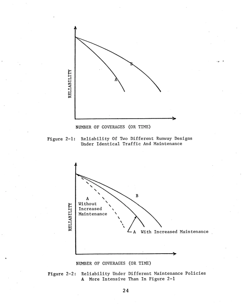
As an example consider two runways A and B. A has been designed for a traffic of.1000 coverages of aircraft having Equivalent Single Wheel Loads (ESWL) of 30,000 pounds. Whereas B was designed for the same ESWL's but for 2,000 coverages; i.e., construction effort or quality is higher for B than A. If we assume that the traffic and maintenance for each pavement is identical, reliability might be plotted as shown in Figure 2-1, Without making definitive statements

concerning failure, it is apparent that as each runway accumulates traffic, the probability of failure increases.

Provided that the ultimate objective of each runway is to supply a pavement having a specific service level for 2,000 coverages, it is clear that the probability of A remaining at the desired serviceability level falls off more rapidly than does the probability of B. Hence, one sees that each runway provides service to the user but that the

reliability of that service is different.

This example has shown a comparison of two differently designed runways under identical maintenance operations. An alternative to the provision of more construction effort lies in maintenance or

main-tainability considerations. 2,1,3 Maintainability

Maintainability may be defined as a measure of the effort required during the life of a facility to assure an adequate level of service. The manner in which this required effort is expended is

termed maintenance. And, it may be divided into two categories, normal maintenance and corrective maintenance. Normal maintenance is of a preventive nature. Generally, it is composed of programmed activities which accomplish certain tasks at a given rate; e.g. sealing 75% of all

cracks once a year. Corrective maintenance in contrast is an unscheduled activity. It is undertaken when a portion of the facility has failed or failure is impending; e.g. replacement of asphalt where a disabled

aircraft has torn away a portion of the pavement.

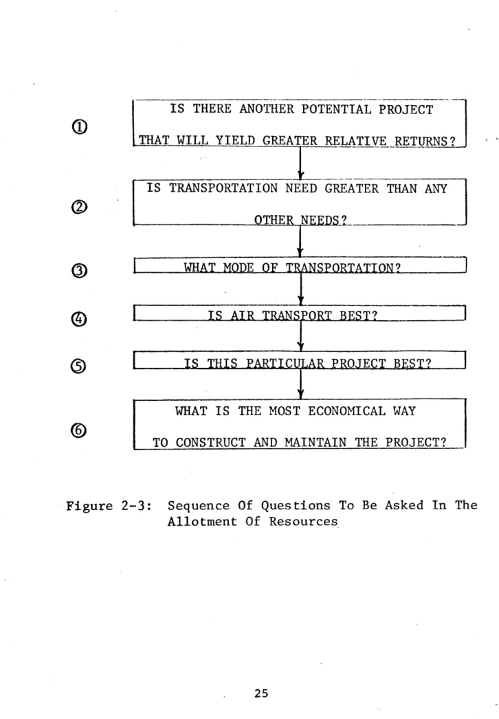
In general, corrective maintenance cannot be accurately planned. Conceptually, more intense normal maintenance may or may not effect the potential need for corrective maintenance. Nonetheless, the proper planning and application of normal maintenance can effect system reli-ability. Consider the above example of runways A and B. The

reliability of these two pavements could be made to approach each other under proper maintenance policies. That is, A could attain a higher reliability, if it were subjected to a more comprehensive maintenance policy. For example, if the maintenance policies had been;

A - Patch .50% of all cracks Seal 40% of all cracks

Fill 60% of depth of all ruts B - Patch 20% of,all cracks

Seal 10% of all cracks

Fill 0% of depth of all ruts

then the corresponding reliabilities might approach each other, Figure 2-2.

Alternatively one could view A and B as having identical design and traffic, but with different maintenance policies, B more intensive than A. In this case Figure 2-1 could be viewed as a likely represen-tation of reliability.

Another implication of Figure 2-1 concerns the relation between construction effort and maintainability. It is noted that A has' lower reliability than B. Hence it may be recognized that in order to

maintain the desired serviceability with a given reliability that more maintenance should be investigated for A.

At this point it should be clear that serviceability, reliability, and maintainability must be considered in the design process.

2.1.4 Performance of Constructed Facilities

Performance of a constructed facility is the embodiment of the three aforementioned components: serviceability, reliability, and maintainability. No system can effectively be evaluated without

recognition of these either implicitly or explicitly. From a structural integrity view, performance lends itself fairly well to evaluation. On the other hand, from a user's psychological perspective the evaluation is much more difficult, As was mentioned earlier, vibration and noise effect the direct user, but to what extent this influences the users perceived utility is difficult to judge. Even more difficult to evaluate, is the relationship between the vibration level the user experiences and the structural integrity of the pavement. In order to begin this evaluation much work is needed in the fields of psycho-physics

and pschometrics. The detailed examination of these fields and their implications is somewhat outside the realm of this thesis. (For a comprehensive explanation of this area see Thurstone (13), Fechner (15), Winkler (16), Galantner (17).) Nonetheless, the maintenance model

deals with these areas in its evaluation and a brief discussion of them is presented in Chapter III.

In analysis and design of systems of constructed facilities, system performance and the economic costs of the facility must be evaluated. Most often the designer's task is to provide some level of performance within some set of cost constraints. Tradeoffs exist between construction cost, maintenance costs, and user cost. Hence it

is economically feasible to evaluate the performance of a system within the context of a total cost analysis.

2.2 ECONOMICS

The planning, design, construction operation, and maintenance of any constructed facility must be considered within the context of a broadly defined environment. Four problem areas should be investigated:

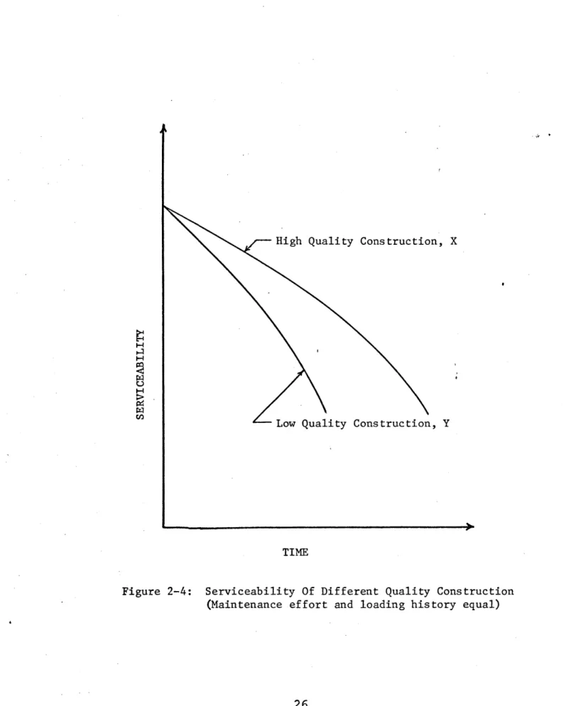
(a) economic, (b) social, (c) political, and (d) technical. One logical manner of attacking these problems is to ask a series of

questions concerning the distribution of resources and the accruement of returns, Figure 2-3. It is assumed that the terms resources and returns may be considered in a broad sense economic but in a more specific

sense social and political,

In this study, it is sought to provide the decision maker with a tool which will aid him in answering questions

G

evaluation of the costs involved: construction, maintenance, and user. 2.2.1 Total Cost of Service

Several alternative methods of economic analysis are available: (a) equivalent uniform net return, (b) net present value, (c) benefit/ cost ratio, (d) equivalent uniform annual cost, and (e) internal rate of return (for a thorough treatment of these see Samuelson (12), Baumol (18), Grant and Ireson (19), or Winfrey (20), The method proposed for evalu-ation of costs in this study is present value of total costs.

Present value of total costs is a particularly attractive method in that it allows not only the evaluation of construction costs,

maintenance costs, and users' costs; but it also provides the decision maker with a time stream flow of resources - costs. This last aspect may be of substantial importance in that it allows consideration of

expenditures of future resources as balanced against projected avail-ability of these resources. It is evident that the benefits of the total cost technique are lost if any of the components of cost are deleted or misjudged. In previous years the components, construction cost, and user cost have received much attention, Consequently,

several sophisticated techniques exist which allow close approximations of their values. (See Manheim, et. al. (21)). Contrastingly, the estimates of maintenance cost, when not omitted entirely, have relied on what can only be termed "experience". Several objections to these estimates exist, Two of these are:

1. The facility for which the estimate is rendered must already exist in

order for experience to be gained.

2. In order for estimates to be made for a proposed facility,

a similar facility must exist in a similar environment.

Of course several other objections concerning changing traffic and

changing maintenance policies exist. Consequently an accurate mechanism for maintenance estimation will be desired.

2.2.2 Details of Total Cost Evaluation

The formula used for the evaluation of present worth of total cost is:

TC = j n CC.. + MC.. + UC.. (2-1)

j "1 1 i 1J

(1 + d)

where TC. = Present worth of strategy i over an analysis period of

1

j years

CCij , MCI., and UCij = respectively

construction, maintenance, and user costs predicted for strategy i in year j.

d = discount rate or the opportunity cost of capital By this method, the strategy with the lowest present worth of total service cost is preferred (22). Hypothetically, this technique could be expanded to include costs associated with political and social effects. However this does not appear practical. Nevertheless the

total cost approach can yield costs for the facility which are required in the evaluation and comparison of different projects within a broad framework.

From the total costs perspective the components of maintenance costs and user's cost do not necessarily remain equal for two different construction efforts. (It is assumed that more construction effort requires increased construction costs.) In fact many combinations of

construction costs, maintenance costs, and user costs are possible. It was shown in the preceding section concerning performance that

combinations of maintenance and construction effort may result in facilities which have equal reliability. Furthermore, it can be shown that these components effect the serviceability of the facility. In this respect it should be recognized that interaction among the cost components is not independent. Hence this leaves the way clear for consideration of'

tradeoffs among the three.

2.2.3 Maintenance-Construction Costs

Intuitively, one may assume that low maintenance costs are

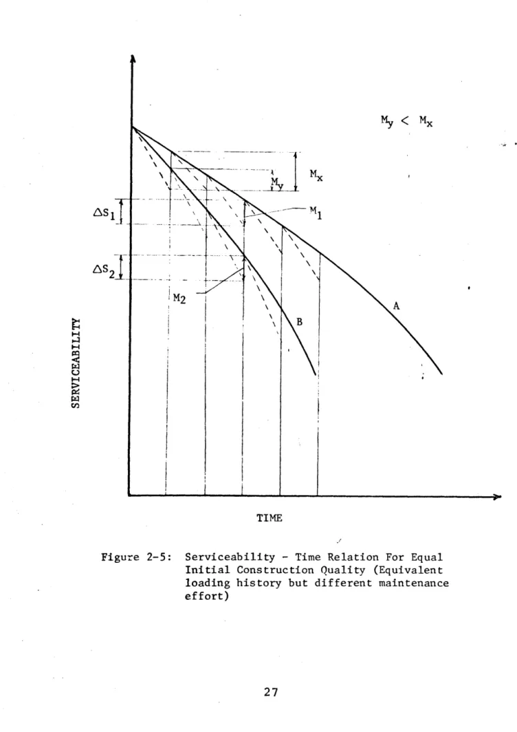
associated with high construction quality. Conversely, high maintenance expenditures should be required for projects having low construction quality. These maintenance-construction relations are most nearly true for projects which must meet similar serviceability requirements within equivalent economic environments. Figure 2-4 shows a relationship

between two projects which must meet similar serviceability requirements with time. Apparently the low quality construction could have approached

the serviceability history of the high quality construction if more maintenance effort had been expended. Furthermore, it could be shown

that the service life of X could have approached that of Y had a smaller maintenance effort been expended on X.

On examining the effects of different maintenance efforts for projects having equal construction quality, Figure 2-5, it can be seen that the serviceability histories of A and B are considerably different. By relating S1, 6S 2 (change in serviceability - improvements) and M1, M2 (maintenance effort), a maintenance cost-improvement relation can be proposed similar to Figure 2-6. For this relationship it is assumed

that a higher maintenance effort (M > M2) regains a larger value of serviceability (SSI > AS2). Presumably M1 is more expensive than M₂.

It should be noted that the relationship of Figure 2-6 is valid for only one time period. Even though later time periods will require Z Sx improvements equivalent to previous ASS's, the cost will not necessarily be the same. This difference is related to the method of

achieving a specific 6 S through a maintenance effort M , i.e.,

x x

Mt #* Mt-1 Mt+1 even though ZS t = t1 = St+1 because the

maintenance operations for Mt, Mt-1 , and Mt+1 may be entirely different.

Consequently, the associated costs of repair will be different. Hence, the representation of the relationship between maintenance effort and improvement requires a family of curves as shown in Figure 2-7.

If one wishes to also associate maintenance effort and improvement with construction quality, another family of curves will be needed as

shown in Figure 2,8.

The foregoing serviceability, construction quality, maintenance effort interactions show some of the complexity involved in designing, constructing, and maintaining constructed facilities. These interactions have special significance for runway pavements because they allow the designer or maintenance manager the alternative of meeting service level requirements in several different ways,

2.2.4 User Costs

The maintenance-construction tradeoffs discussed above concern themselves with equivalent serviceabilities. That is, there are combinations of construction effort and maintenance effort which can provide similar serviceability histories (performance). In this respect

the user will experience no change in his cost. However, if the service level differs from strategy to strategy the user's cost will vary.

Explicity this means that no trouble occurs when using present value of total costs for comparing projects of similar performance.

In contrast, modifications must be made if the service level varies. Implicitly, varying levels of service are accompanied by changes in user costs. And unless the facility is subject to an inelastic demand for service, the number of users will change. To some extent, large

metropolitan airfields represent facilities having an inelastic demand for service. Whether the runways are in poor condition or excellent condition, the same number of aircraft will seek to land. This obser-vation is made under the influence of present capacity operations at many of this nations air transport hubs. There exists the probability

however, that the inelasticity of this demand cannot be extrapolated into future years, Prediction concerning demand must consider that new airfields are under construction (and existing fields are undergoing reconstruction) and will enter the air transport market in a competitive manner. Furthermore, it is evident that the inelasticity of the

demand has limits, i.e. after a certain user cost is passed other modes of transport will become more popular and more competitive. Therefore the decision maker must have some methodology for establishing service levels and thereby user costs.

A modification of equation 2-1 will allow consideration of

various service levels together with maintenance and construction costs under changing demands. It is suggested that the concept of willingness to pay be used in the modification of the present worth of total costs technique.

A thorough treatment of this evaluation is not essential here. Thus the reader is referred to reference (20) for a more detailed description.

2.3 SUMMARY

For a given level of serviceability there exist many combinations of maintenance and construction effort which will provide the desired performance. For each combination considered there are costs associated with construction and maintenance. It has been shown in section 2.2.3 that maintenance costs and maintenance efforts vary with construction quality. In fact even though the same change in serviceability may be desired for two different projects or at two different times the

maintenance model computer program which is described in the next chapter allows tradeoffs between construction and maintenance to be examined in

terms of service, damage, and maintenance costs. While the model does not allow the specification of AS's it does allow the evaluation of the resulting costs and performance under specified maintenance efforts, M's. This means that those relationships that are discussed in section 2.2.3 have been established, but in reverse of the manner described therein

(i.e. M's are specified and AS's are evaluated and output in combination

with the service level after maintenance).

The concept of a total cost evaluation has been introduced to show how different combinations of construction and of maintenance may be evaluated by the decision maker (i.e. planner, designer, maintenance manager, operator). The third component, user costs, should have no

significant effect upon the total cost decision unless changing levels of service are to be considered. The actual evaluation of user cost is not a part of this study. However it has been discussed because it forms an integral part of the proposed economic evaluation technique; and hence must be considered in any meaningful economic evaluation.

It should be apparent now that the intent of this study is not to formulate a decision making model. Instead the purpose of this study is to present both in concept and in detail a tool which can aid the

decision maker in his task. This tool should be able to predict costs and performance which will allow decisions to be made more effectively within a broad environment involving not just technology and climate but

also politics, economics, and society.

NUMBER OF COVERAGES (OR TIME)

Figure 2-1: Reliability Of Two Different Runway Designs Under Identical Traffic And Maintenance

Maintenance

NUMBER OF COVERAGES (OR TIME)

Figure 2-2: Reliability Under Different Maintenance Policies A More Intensive Than In Figure 2-1

IS THERE ANOTHER POTENTIAL PROJECT

THAT WILL YIELD GREATER RELATIVE RETURNS?

IS TRANSPORTATION NEED GREATER THAN ANY

OTHER NEEI S

WHAT MODE OF TRNSPORTATION?

IS

AIR

SPRT

BEST?

IS THIS PARTICUAR PROJECT BEST?

WHAT IS THE MOST ECONOMICAL WAY

TO CONSTRUCT AND MAINTAIN THE PROJECT?

Figure 2-3:

Sequence Of Questions To Be Asked In The

Allotment Of Resources

High Quality Construction, X

Low Quality Construction, Y

TIME

Figure 2-4: Serviceability Of Different Quality Construction (Maintenance effort and loading history equal)

\s

My < M

B

TIME

Figure 2-5: Serviceability - Time Relation For Equal Initial Construction Quality (Equivalent loading history but different maintenance effort)

27

0 o --I H o Pr4l 6S ₁ AMOUNT OF IMPROVEMENT -Initial Serviceability Or Quality I _____________ SS _max

Figure 2-6: Maintenance Cost - Improvement Relation (AS denotes increment of improvement)

-Initial Serviceability Or Quality

Smax IMPROVEMENT

Figure 2-7: Maintenance Effort - Improvement Changes With Time, T.. (Relationship assumes equivalent loading and initial quality of construction)

Low Initial Servicea ility

Low Initial Quality

High Initial Quality

High Initial Servic ability

IMPROVEMENT, A S

Figure 2-8: Maintenance

-

Improvement With Varied Maintenance

Effort And Initial Construction Quality

CHAPTER III

THE MAINTENANCE MODEL

The maintenance model described in this chapter forms the central portion of this thesis. The chapter is divided into two

sections. Section 3.1 deals with the model concept. It notes both the need for stochastic modeling as well as the empirical nature of the

current model. The detailed description of the airfield pavement maintenance model follows in section 3.2. This section discusses the relations which were chosen for simulating pavement deterioration and maintenance and their operation. The operation of the model is explained

by the use of an example. 3.1 MODEL CONCEPT

The driving motivation for maintenance operations is to maintain adequate serviceability at a desired level of reliability. In the model concept developed herein, serviceability, reliability, and

maintainability are not input parameters. Rather, the model evaluates proposed or existing designs in a specified climate and traffic environ-ment and yields indications of these performance parameters. These indications take the form of estimates;

1. Estimates of the condition of the runway/taxiway pavement;

2. Estimates of the maintenance efforts required to change conditions;

3. Estimates of the associated costs with changes.

Ideally the performance of the pavement could be shown as Figure 3-1. The performance, P, as shown can be related to damage, D, in the pavement. If P and D are fractional quantities and hence range in value between 1.0 and 0.0 inclusive, a relationship between them may be

established as a function of time or traffic.

where t = traffic or time at t = 0.0, P = 1.0

and at P = 0.0, t = time at end of service life, D = 1.0

This is the concept upon which this work is based. 3.1.1 Ideal Structural Concept of Model

In concept the model should evaluate the existing or planned airfield pavement construction and yield estimates of its performance. From the point of view of the supplier (planner, designer, operator, maintenance manager, etc., ) and user the amount of damage or

deterioration and the level of serviceability are important. Hence it appears that the complete evaluation of this constructed facility may require at least two transfer functions, T and U. Where T (Y.) relates some set of structural design properties, Yi's, to the future pavement response (damage or deterioration) which the facility will exhibit under a predicted climatic and traffic environment. Once this response

is predicted the U(X ) function evaluates the damage or deterioration measures, Xits, and predicts the reaction of the user. Parameters in

the Y. set include materials properties, pavement geometry, climate, and

1

traffic. While the X. set may be composed of such damage characteristics

1

as cracks, ruts, and roughness. This is the technique which is proposed in the ideal and current model. At first a deterministic solution of T and U seems applicable, however a stochastic approach is more

reasonable (23).

The stochastic approach is preferred due to the probabilistic nature of the pavement and user responses. It should be noted that the

observed response (damage) of the pavement structure depends upon the probabilistic nature of loading rate effects (24, 25), the position and magnitude of the applied load (26), climate (27), materials type (26), previous traffic history (26), temperature (26), and construction variables (28). Furthermore the perceived utility of the users will

The ultimate objective of the pavement facility is to provide service to the user. The interim objective of this study is to

yield estimates of maintenance cost and the associated maintainability and reliability. To associate these objectives with the desired

results and format of a model, an ideal strategy must be formulated. First it is desirable to break the problem into its component parts. These parts include input, damage evaluation, aircraft response, and user response. This division implies a linear structure in which each successive component of the system responds to the preceding component. In the simulation model this simply means that responses are calculated step by step. The generalized ideal model might operate as follows:

a. Input pavement design parameters b. predicted climatic environment

c. predicted traffic

d, response characteristics of aircraft e. response characteristic of users f. calculate damage response of pavement

from traffic and climate

g. response of aircraft to runway h. response of user to aircraft

Superimposed on this process are maintenance activities and maintenance cost routines. In flow chart form the total process might appear as Figure 3-2.

Recall that it is most desirable to investigate stochastic modeling for this system, This implies that a certain knowledge of system

variables exists. The knowledge should include not only material

properties but their accompanying distributions for the pavement system. For the user the response character of cargo would be needed as well as the response character of passengers and crew. These relations require not only a great deal of data but also a reasonable understanding of how

the components of the system interact.

At the first level of interest, the pavement, it has been pointed out that many factors effect its structural response and/or

damage. Elliot (29) has made the following observation: "... the indicators of structural inadequacy are the manisfestations of the physical failure of the facility, in the particular load, temperature and material property environment. It is therefore pertinent to ask whether analytical models, mathematical or otherwise could be found to account for the manner in which a particular load-temperature-material property-environment would effect the performance of the layered

structure." The author of the present thesis knows of no such all inclusive model in operational existence at the present time (1971). Likewise models for aircraft response and user response are required. One model by Tung, Penzien, and Horonjeff has particular promise for predicting airframe responses (30). Furthermore a model by Coermann (31) may be used to predict the.physical response of human users in the

aircraft. The most well developed model is the aircraft response model while the user model is perhaps the least developed. Obviously the user

response is a difficult evaluation in that physical and pschological models are required.

Even though many problems are apparent a rational simulation and evaluation of the responses of the several system components may be proposed within the ideal framework of Figure 3-2. Three submodels are

required (a) pavement, (b) aircraft, and (c) user. In connection with each of these the author has found three models which may, after much work, be combined as a total rational model. Ashton (32), Elliot (33),

Findakly (34), and Soussou (35), have all worked on stochastic models of the viscoelastic nature of bituminous pavements. The work to date has not resulted in a final damage model but it promises to in the near

future. The aforementioned model by Tung et. al. (30) has much promise. It is formulated as a deterministic model. Response of the airframe in terms of vibrations and acceleration may be predicted. The third

model needed is one which simulates user response. Assuming that human response is most critical (i.e. cargo response can be altered by

packing techniques) the model of the human body by Coermann (31) may be used. This model presently has the limited capability of predicting

average physical responses. By a thorough investigation of human response to motion (vibration and acceleration), the fields of

psychology and human factors might be used to derive a rational user response function. At the outset of this study none of the three models mentioned were in suitable form for incorporation. However the rationale which surrounds these has been thoroughly investigated and where appropriate utilized, Hence due to the present shortcomings of the

above an empirical technique is used. 3.1.2 Current Model

The current model is not viewed as a completed study but as an interim tool. In its present form it should be able to aid two groups

(a) researchers and (b) designers and maintenance managers. With some additional work in the area of comparison and calibration, it is thought that the model, as it exists, may be used as a tool for the designer and maintenance manager in the area of service life prediction and

maintenance planning. The researcher should find the interactions which occur in the model instructive and helpful.

3.1.3 Basic Relationships

Before dealing in detail with each component of the program, the essential relationships between pavement, aircraft and user should be presented. The predominant pavement factor of interest is macro-roughness or surface unevenness (14, 36-44)*. Pavement roughness, defined as

deviation from a smooth flat horizontal surface, causes several modes of movement or vibration, vertical, horizontal, and angular, in the

airframe (30, 42, 44). These vibrations together with their amplitude have been shown through human factors research (14,36,37) to effect the users perception of comfort and/or safety. Therefore the two parameters which this study is most interested in are roughness and vibration.

*Macro-roughness does not include skid resistance problems which are of a smaller scale and termed micro-roughness. For a thorough review of skid problems and their possible solution see Dahir (45).

3.1,4 Performance Concept

The components serviceability, reliability, and maintainability may be examined with the model. Measures of service are derived by investigating the vertical acceleration to which the passenger is

subjected. Maintainability may be inspected through the service level-time relationship which results with changes in maintenance policy. And reliability can be checked by comparing the service behavior of the facility under equal traffic and environment but with different main-tenance and construction strategies (see section 2.1.2).

It should be recognized that with these capabilities the model not only approaches the ideal concepts but that it becomes a useful tool to those experienced in airfield maintenance.

3.2 DETAILED DESCRIPTION OF MAINTENANCE MODEL

The preceding section, 3.1, has shown that the maintenance model is based upon the concept that damage and performance are related. This implies that if one can be predicted the other can be determined. In section 3.1.1 it has been pointed out that it is desirable to

determine some functions T and U which allow first the prediction of

damage (as a function of materials properties, pavement geometry, climate, and traffic) and secondly the prediction of user response. Relation-ships which allow these determinations are formulated in the current model. These relationships have been used in programming an airfield pavement maintenance computer simulation using the Fortran IV computer

language (46). Basically the computer program performs four functions: 1. Simulates deterioration of the

pavement by predicting the change in roughness as a function of traffic and environment.

2. Predicts changes in serviceability with changes in roughness.

3. Estimates changes in roughness as a function of maintenance policy.

4. Estimates quantities of labor and material and costs for a specified maintenance policy.

The structure of these functions within the program is presented in Figure 3*z3.

Each of the four individual functions are described in detail within this chapter, Furthermore, at the end there is included a brief summary of the required input and expected output of the program.

3.2.1 Deterioration

The primary value to be considered in deterioration is surface roughness, It has been shown that roughness may vary linearly with both the weight and number of applications of traffic (47,48,49). Nevertheless one realizes that an aircraft having a weight of 100,000 pounds per

landing gear effects this deterioration of the pavement differently than one having 30,000 pounds per gear. The approach used in this study concerns the equating of some common measure of traffic to a measure of damage (50-54). Therefore derivation'of equivalence factors which allow the reduction of several different loading conditions to a common

denominator is desirable. The Corps of Engineers pavement design method has been used in the derivation of these equivalence factors (55-59).

Considerations for pavement properties and traffic may be represented by (47,55,60,62):

1. Subgrade support

2. Equivalent pavement thickness (60) 3. Equivalent coverages*

The Corps of Engineers' thickness design equation allows the investigation of the interaction of these parameters.

*"a coverage occurs when each point on the pavement surface has been subjected to one maximum stress by the operating aircraft" (61).

P P

t = (0.23 log C + 0.15) P

8.1 CBR p (3-2)

where: t = thickness of flexible pavement structure

C = traffic volume, (coverages)

P = wheel load, (single or equivalent single wheel load, ESWL - pounds

CBR = soil strength measurement, (California Bearing Ratio)

PC = tire inflation pressure, (psi). Equation 3"2 may be rewritten in terms of coverages:

C =

lw

where w = B t _{P P.} -0.15 _0.231

I8.1 CBR P0

C

With equation 3-3 equivalent coverages may be determined via equivalence factors, EF, as derived in equation 3-4 and shown schematically in

Figure 3-4.

EF = Cta _(3-4)

C

Where:

EF = Equivalence factor

Cta = Coverages to failure for the aircraft for which the pavement was designed

C = Coverages to failure for any aircraft, x other than the type for which the runway was

designed.

To account for climatic influence, subgrade support during the spring thaw period was considered. An environmental factor, ENVFT, was

derived from Asphalt Institute (62) and Road Test Research (63). ENVFT = log_{1 0} log_{1 0} CBRdesign CBR spring

Both the equivalence factor, EF, and the environmental factor, ENVFT, are used to determine the total number of equivalent coverages per year (see Figure 3-4).

The following example best explains the equivalent loading calculations. EXAMPLE Given Number of Coverages/Year 100 100 100 100 100 100

Equivalent Single Tire InflatiQn Wheel Load* (kg.) Pressure ( Kg/cm )

28636 30909 30909 15909 18181 41818 10.6 11.6 11.6 9.2 10.2 12.7 Pavement Thickness = 71cm. Design CBR = 10.0 Spring CBR = 7.0.

*Determined by Corps of Engineers Method (56,57).

(3-5) Type Aircraft 1 2 3 4 5 6

Findings For Loading Only Coverages to Failure CFAIL(I) 13,954 8,354 8,354 774,284 247,691 1,780 Equivalence Factors 1.0 1,67 1.67 0.018 0.056 7.84 Equivalent Coverages For Year 100 167 167 1.8 5.6 784

Total For Year = 1, (TOTAC) = 1225 coverages

Determine Total, With Environmental Factor

Given 1. SPTHW, % of traffic during spring thaw period SOLUTION 1. Determine number of equivalent coverages during

spring thaw, SPRNG

SPRNG = Total For Year, (TOTAC) x SPTHW

2. Determine ENVFT, Environmental Factor

ENVFT = logl0 DESIGN CBR logl0 SPRING CBR

= logl0 10 logl0 7

= 1.18

3. Determine total corrected equivalent loadings for year, YTOTL

YTOTL = (TOTAC - SPRNG) + (SPRNG X ENVFT) YTOTL = 1270 Coverages

The next step after calculating the equivalent loadings for the year involves determining the amount of associated roughness. As was previously noted the deterioration-loading relation can be represented as a linear process. This of course implies that a sharp increase in traffic will be accompanied by a similar rise in roughness.

All the traffic in the example has been converted to equivalent coverages of aircraft type 1, CFAIL(1). Thus the change in roughness, RCHNG, for the example may be determined.

RCHNG = (YTOTL/CFAIL(1)) x 158cm/km (3-6) where:

RCHNG = change in roughness, cm/km

158 = range of roughness variation in cm/km New construction = roughness = 79 cm/km

Failed condition = roughness = 237 cm/km. (64) YTOTL = Total environmentally corrected equivalent

coverages for year, equal to 1270 for the example

CFAIL(1) = coverages to failure of aircraft type 1, equal to 13954 coverages in the example Therefore RCHNG for one year is

RCHNG = (1270/13954) X 158 = 14.38 cm/km.

Hence the roughness at the end of year 1, before maintenance is: Roughness = 79.0 + 14.38 = 93.38 cm/km

The reader should refer to the flow diagram of the current model Figure 3-3. From here it can be seen that the foregoing process can be

repeated in part or in full for each year of analysis. 3.2.2 Serviceability-Roughness

Work by Hutchinson (14), Goldman (36), and Parks (37), and others leads to the concept of roughness related serviceability. It is seen from much of the work done by NASA (65), ALPA (66), and the U.S. Corps

of Engineers (67) that pavement roughness directly effects vibration of both the human and mechanical systems which traverse the runway/taxiway. Vertical vibration is considered the most critical case.

Human response to vertical vibration may be characterized as shown in Figure 3-5. The range of frequencies from 0 cps to 20 cps is particularly critical because man's natural capacity for vibration

absorption is least effective in this range (14). For this first model a serviceability relation is formulated by investigating vertical

acceleration (VA) in the 5 cps range.

Establishment of an arbitrary measure of serviceability, as in the AASHO Road Test, (63), may tend to limit the utility of the model. Consequently, the model predicts and evaluates vertical acceleration, VA, as a function of roughness. This procedure is more generally useful in that it will allow consideration of the pavement serviceability to the airframe, cargo, instruments, crew, and passengers. In these

early stages of development the model is used to evaluate serviceability in relation to human response. Since the major concern at this stage is service to the passengers and crew; a safety criterion was chosen in connection with failure. The failure state is defined as that condition at which the VA Z 0.7g because it becomes extremely difficult for the pilot to carry out his duties safely at this amplitude of vibration (especially in the 5 cps to 20 cps range of interest in this study) (14,40).

The shape of the acceleration-roughness deterioration curve (Figure 3-6B) may be determined by considering a variety of runway profiles with their accompanying roughness and acceleration measures. Actual comparison of runway roughness and resulting vertical acceleration has not been undertaken in this study. Rather the relationship has

been assumed. It is noted that normal bituminous pavements vary from a roughness of 50 inches/mile (79 cm/km) to 150 inches/mile (237 cm/km) from their newly constructed to their failed states respectively (64). Equation (3-7) is the result of associating O.lg and 1.0g vertical acceleration with these roughness measures and assuming a linear

relationship for intermediate values (see Figure 3-6C). VA = -0.35 + 0,0057 R** (3-7)

where:

VA = vertical acceleration in gTs R = roughness in cm/km.

The foregoing allows two relations to be considered: 1. effect of number of equivalent coverages

and climate on roughness; and

2. effect of roughness on vertical acceleration. 3.2.3 Maintenance-Roughness

As roughness changes so do the associated modes of deterioration; rutting and cracking. With the aid of Road Test damage data (63,67) and regression analysis (68), the form of equations '3-8 and 3-9 has been determined.

CP = 627.9 + 89 /0.633 R** (3-8) RD = ~26.7 + 0.338 R + 0.335 TCJ** (3-9) where:

CP = Cracking plus patching, m2/1000m2 R = Roughness, cm/km

RD = mean rut depth, cm

These equations permit the model to estimate structural deterioration with changing roughness. The next step requires the determination of the change in roughness as associated with maintenance effort,

**Equations noted by ** are the result of empirical relations or regression analysis. The units often do not work out properly. In these cases the reader may imagine the components to be multiplied by some unit factor Q which will yield the specified units.

equation 3-10,

R = 79.0 + 2.96 RD - *iP (3-10)

where:

RD and CP are repaired quantities.

To illustrate the simulation of maintenance operations as a function of deterioration and specified maintenance policy consider the following:

NA =[(CP)x - (CP)x_j X WOS X LOS X 1000 m/km (3-11)

where:

NA = area of new cracking on the pavement section, m2 WOS = width of section, m

LOS = length of section, km

The maintenance policy for sealing and patching are specified as fractions of new cracking that will be sealed or patched.

SMS = FTS x NA (3-12)

SMP = FTP x NA (3-13)

where:

SMS = Area sealed, m2 SMP = Area patched, m2

Specified in maintenance policy FTS = fraction of NA to be sealed FTP = fraction of NA to be patched Now the new area of cracking after maintenance, NA', is given by

NA' = NA - (SMS + SMP) (3-14) 3.2,4 Maintenance Quantities and Costs*

To transform the quantities of maintenance required (in this case

*This portion of the program is taken from the previous work of Alexander (22). The explanation is altered only slightly from the original.

square meters of sealing and patching) to quantities of labor, equipment and materials is fundamentally a problem in engineering estimation. This part of the model may be thought of as an automated estimating

procedure. Productivity and consumption rates used in the following equations were determined partly by a review of existing maintenance studies of operational efficiency, and partly from the performance characteristics of the equipment involved.

Hours of labor or equipment time required to accomplish the quantity of work estimated above are determined by functions similar to the following equation, for the equipment hours needed to place patching material.

EHN.. = CCMij x DOP x SMP (3-15)

1J (3-15)

PT₂ 100

In equation 3-15, EHNij represents the hours of j type equipment needed to accomplish i type maintenance operations for the year. CCMij is the hours of j type equipment needed to adcomplish one unit of the i

maintenance operation (in this case, one cubic meter of patching

material), DOP is the average depth of patch placed in centimeters, SMP represents the square meters of patching as determined by equation 3-13 and PT2 is an efficiency factor representing hours actually worked for each hour on the job. This factor can be used to calibrate the model

for the efficiency of the maintenance organization involved. Each type of labor and equipment is estimated by an equation similar to equation 3-15.

Estimating the quantity of materials required is a straight-forward process. Materials estimated are fuel for the maintenance equipment and the actual materials placed on the road during maintenance.

The quantity of fuel required for each type of equipment is estimated from the hours of equipment use previously estimated:

Where MPij represents liters of gasoline required for the j type of equipment to accomplish the i operation: EHNij is determined in equation 3-15 and Cij is the appropriate fuel consumption factor.

It is also relatively simple to estimate the quantity of material placed on the road during maintenance. To continue with the example of sealing and patching, the tons of bituminous patching material needed is found by:

MBA. = DCG x DOP x SMP

i (3-17)

100

where DCG is the compacted density of the finished patch, and the other variables have been previously defined.

After the quantities of labor, equipment, and materials needed for the year have been determined, cost for each quantity is found. The quantities of each item are multiplied by the appropriate unit costs, which are furnished by the model user.

The estimated maintenance costs are subtotaled for labor,

equipment and material. Each of these subtotals is then discounted to present worth values.

The subtotals of present worth cost are then added to find the total, present worth cost for the year. The actual costs are also totaled for each year. These total yearly maintenance costs are accumulated as the model works to the end of the analysis period. 3.2.5 Input-Output

The preceding detailed descriptions have sought to recount the rationale behind the formulation of the current model. It is perhaps unclear just what quantities the computer program requires as input. Furthermore the output quantities may be vague.

Table 3-1 lists both the type of factor and its measure needed as input for damage estimation. Additional input is required for the

maintenance estimating routine. A thorough treatment of the input details is given in Appendix II, User's Manual.

Typical output includes:

(1) the number of equivalent coverages; .(2) the amount of cracking and patching

before and after maintenance;

(3) average roughness for each period or year;

(4) the changes in roughness;

(5) the average vertical acceleration for the year and;

(6) the yearly and accumulated actual and discounted costs,

This output sequence is continued for any one project until either the number of periods of simulation or the allowable vertical acceleration is exceeded, A copy of the output for year 1 of one run is given in Figure

3-7. A more comprehensive description is not included here. However the reader is again referred to Appendix II for a full description of the program's requirements and capabilities.

3.2,6 Review of Details of Maintenance Model

In review, one should again examine the flow of the maintenance model. Figure 3-3 is schematically designed to explain the flow of

operation which the computer model of maintenance follows.

The model provides the designer with the capability to test various combinations of construction quality and maintenance effort.

Furthermore, it permits the designer to test a particular combination of construction and maintenance under changing climatic and traffic demand environments. For maintenance management, the model yields

estimates of the performance consequences of various specified maintenance programs. Maintenance management may also test a given maintenance

policy against varied traffic and climatic environments. In both cases, the model will predict damage and estimate the flows of cash, material, men, and machines under various input constraints as presented in Table 3-1.

One should remember that the maintenance model as presently constructed, will serve as an estimating tool. Consequently, as

experience is gained with its use both the model's accuracy and usefulness will improve,

TABLE 3-1

Input Factors Influencing The Damage Estimation Of Airfield Pavements FACTOR MEASURE 1. Construction Quality 2. Traffic 3, Environment 4. Maintenance Effort ,. (a) (b) 2. (a) (b) (c) 3. (a) (b) 4. (a) (b) (c) Pavement Thickness CBR Of Subgrade ESWL

Tire Inflation Pressure Number Of Coverages CBR - Design

CBR - Spring

Fraction of Cracks Filled Fraction of Cracks Sealed Fraction of Rut Depth Filled

P - Perfqrmance

_%Unacceptable Leve Of Performance

Service Life

TIME OR NUMBER OF LOAD APPLICATIONS, t

Figure 3-2: Flow Chart Of Ideal Concept Of Simulation Model

INPUT: 1. CONSTRUCTION QUALITY

2. ENVIRONMENTAL PARAMETERS

3. TRAFFIC CHARACTERISTICS

4. SPECIFIED MAINTENANCE POLICY

5. MAXIMUM ACCEPTABLE VERTICAL ACCELERATION 6- NO. OF PERTODS OF TEST

IDETERMINE

-OR PERIOD -- EQUIVALENCE & ENVIRONMENTAL FACTORS

PERFORM MAINTENANCE AS PER SPECIFIED

MAINTENANCE POLICY

ESTIMATE COSTS, QUANTITIES, AND ACTIVITIES

FOR PERIOD

I ADD PERIOD COSTS AND OUANTITIES TO ACCUMULATED TOTAL

DETERMINE IMPROVED ROUGHNESS

DETERMINE AVERAGE ROUGHNESS FORP, YEAR i.e.

(ROUGHNESS BEFORE TRAFFIC FOR YEAR

+ROUGHNESS JUST BEFORE MAINTENANCE +ROUGHNESS JUST AFTER MAINTENANCE) / 3

ESTTMATE AVERAGE VERTICAL ACCELERATION

FOR YEAR

ND

NO

-1

Figure 3-3: Detailed Schematic Of Maintenance Model

Additional Loading From

Environmental Consideration

NUMBER OF COVERAGES

NUMBER OF COVERAGES

Figure 3-4:

Schematic Of Equivalent Coverage Function

1