Analysis and optimization of occluder-based imaging

(1)

Analysis and Optimization of Occluder-Based

Imaging

by

Adam B. Yedidia

B.S., Massachusetts Institute of Technology (2014)

M.Eng., Massachusetts Institute of Technology (2015)

Submitted to the Department of Electrical Engineering and Computer

Science

in partial fulfillment of the requirements for the degree of

Doctor of Philosophy

at the

MASSACHUSETTS INSTITUTE OF TECHNOLOGY

September 2020

c

○ Massachusetts Institute of Technology 2020. All rights reserved.

Author . . . .

Department of Electrical Engineering and Computer Science

August 28, 2020

Certified by . . . .

Gregory W. Wornell

Sumitomo Professor of Engineering

Thesis Supervisor

Accepted by . . . .

Leslie A. Kolodziejski

Professor of Electrical Engineering and Computer Science

Chair, Department Committee on Graduate Students

(2)

(3)

Analysis and Optimization of Occluder-Based Imaging

by

Adam B. Yedidia

Submitted to the Department of Electrical Engineering and Computer Science on August 28, 2020, in partial fulfillment of the

requirements for the degree of Doctor of Philosophy

Abstract

Occluders, i.e. opaque objects, can be used in the apertures of cameras to supple-ment or replace a traditional lens. This thesis describes a novel mutual information-theoretic framework for analyzing and comparing occluders. It justifies the use of uniformly-redundant arrays (URAs), a popular choice of occluding pattern in coded-aperture imaging. This thesis shows these patterns to be optimal under ideal con-ditions using this framework. Outside of those ideal concon-ditions, this thesis proposes a method for selecting between different URAs and compares it to other occluder-selection methods, such as a greedy search, identifying under which conditions each is preferable. It also shows, analytically and empirically, the superiority of designed occluding patterns like URAs to random occluding patterns. The mutual-information theoretic framework is compared to a similar, MSE-minimizing framework.

This thesis also considers the use of occluders in the context of non-line-of-sight (NLoS) imaging, used as “accidental cameras.” The idea of the accidental camera is to opportunistically make use of occluding objects that happen to be available as ad-hoc coded apertures. Methods of this class, having originally been developed by Torralba and Freeman in 2012, are extended in this thesis to a wide variety of different scenarios, and used to solve formerly unsolved NLoS problems. These include imaging around a corner using the corner as the occluder, imaging a light-field of an unknown scene using a known, calibrated occluder, and imaging an unknown scene using an unknown occluder. The tools of the aforementioned framework are used to draw tentative conclusions about NLoS imaging systems, including resolution limitations due to longer light wavelengths and the quality of reconstructions across different systems.

Thesis Supervisor: Gregory W. Wornell Title: Sumitomo Professor of Engineering

(4)

(5)

Acknowledgments

First and foremost, I’d like to thank Gregory Wornell, my research advisor, for his invaluable help, ideas, and for the home he gave me at MIT. Without him, I never would have been introduced to the research topic of non-line-of-sight imaging, which plays a central role in my thesis. Everybody always says that choosing an advisor is the most important part of graduate school; it warms my heart to say that they were absolutely right.

I’d also like to thank the rest of my thesis committee, Bill Freeman and Frédo Durand, who met with me regularly throughout my PhD and whose ideas, support, and discussions were tremendously useful. I’d like to especially thank Bill Freeman for his mentorship and generosity with his time and attention; it was thanks to him that I found a postdoctoral assignment during the dreadful time of COVID-19. Bill Freeman’s boundless creativity will forever inspire me.

I’d like to thank Martin Rinard, who co-advised me at the start of my PhD, for his tremendous generosity, kindness, and liveliness. Martin gave me a home when I first came to graduate school, and he funded me before I was covered by my NDSEG fellowship. My research went in a different direction over the course of my PhD, but I have not forgotten his generosity, nor will I.

I’d also like to thank Phillip Stanley-Marbell, for taking me under his wing at the start of my PhD. He was ludicrously nice to me. I didn’t know people could be that nice. He and Max Shulaker mentored me during my ill-fated foray into hardware design, and I will always remember their incredible kindness.

I’d like to thank Regina Barzilay for introducing me into her group, and for the opportunities she gave me to work with all the people at MGH.

I’d like to thank all my co-authors over the course of my PhD: Miika Aittala, Ganesh Ajjanagadde, Manisha Bahl, Manel Baradad, Regina Barzilay, Katie Bouman, Richard Brent, Frédo Durand, Bill Freeman, Connie Lehman, Andrea Lincoln, Nick Locascio, Lukas Murmann, Prafull Sharma, Christos Thrampoulidis, Antonio Tor-ralba, Greg Wornell, Vickie Ye, and Lili Yu. A few of these I would like to thank in

(6)

particular.

Richard Brent answered an email from me, a stranger emailing him out of the blue. Working with him was a great pleasure. I am extremely grateful to him.

Christos Thrampoulidis mentored me throughout the middle of my PhD. His advice and mentorship made me grow tremendously as a researcher—and even more importantly, Christos is a lot of fun to be around.

Ganesh Ajjanagadde and I had countless stimulating conversations. Ganesh is tremendously generous with his time and his ideas, and I could not have asked for a better person with whom to share my time in graduate school.

And then, of course, Andrea Lincoln. I’ll get back to her.

I’d like to thank Tricia O’Donnell, for the endless things she did for me over the last five years. She was always there, always helpful, and always cheerful, even after I messed up.

I’d like to thank Janet Fischer, for all the help she’s given me over the course of my PhD.

Most of my research was funded through a DARPA grant and an NDSEG fellow-ship. I am grateful to both organizations for making my research possible.

I am grateful to all my friends, from Epsilon Theta and from elsewhere, sadly too many to name. But Alex Arkhipov and David Farhi deserve particular mention for providing lots of useful advice about my research, some of which made it into this thesis. And Sam Bankman-Fried, as well, for giving me good advice about grad school and life in general.

I am deeply, deeply grateful to my family: Ann Blair, Jonathan Yedidia, and Zachary Yedidia, and the uncountable things they’ve done for me. I know how lucky I am.

Finally, I’d like to thank my fiancée, Andrea Lincoln. The story of my PhD— indeed, the story of most of my adult life—is in large part a story about her as well as me. She is the best part of my life, an uncomplicated good. She is part of who I am now, and I am deeply proud of that. I can’t possibly describe all of what she is to me here—nor should I—but Andrea is my partner, lover, best friend, and confidante.

(7)

Relatedly, I’d like to thank Virginia Vassilevska-Williams and Ryan Williams. I know what they did for me, even if they may not.

(8)

(9)

List of Figures

1-1 The earliest surviving photograph, taken by Joseph Nicéphore Niépce in 1825, using an occluder-based camera. . . 36

1-2 This figure will appear again, later in this thesis, when more context with which to understand it has been given. The point here is that when the simulated unknown scene (top middle) is projected through a pinhole occluder (top left), it results in a more intelligible projected image, or “observation” (middle left) but a lower-quality reconstruction of the scene (lower left). In constrast, when the simulated unknown scene is projected through a more complicated occluder, in this case a uniformly redundant array (top right), it results in a less intelligible projected image (middle right) but a higher-quality reconstruction of the scene (lower right). It makes sense that historically, the simpler (left) approach would be the first, because no computation is required to understand the observation, but the more sophisticated (right) ap-proach is more powerful. . . 38

(14)

1-3 A hypothetical scenario in which occluder-based techniques could be used for non-line-of-sight imaging. On the left, we can see a door, but we don’t know anything about what’s in the room it leads to (shown on the right). Together, the door and the chair inside the room form an accidental camera. Using the method presented in Section 4.5, an onlooker could, in principle, try to reconstruct an image of the room by observing the door by using the occlusion provided by the chair and the motion provided by the person. This is true even though neither the chair nor the person is visible to the onlooker! I say “in principle” because in practice, the signal strength in the room as shown would be too weak to get a sharp reconstruction—this is meant as an illustration of what is possible with accidental cameras, not a description of current capabilities. . . 40

1-4 Imagine you are in the blue car, approaching the intersection ahead. There’s a green car headed towards the intersection around the corner, but you can’t see it, because there’s a building blocking your view. However, the green car is reflecting green light onto the street in front of you, and that green light is something that is within your field of view, even if it’s too faint to be seen with the naked eye. The intersection in front of you, combined with the building to your left, form an accidental camera. An automatic driving system could use it to infer the angle from the corner and the speed of the green car around the corner using the computational imaging techniques described in Section 4.1. Systems like these could be used to avoid a deadly collision, if the green car is about to run a red light. . . 41

(15)

1-5 A diagram illustrating the following configuration: a point light source at (0, 𝑦𝑝), with a Lambertian surface at 𝑦 = 0. We are interested in the

resulting illumination pattern on the Lambertian surface; to investigate it, we measure the illumination of a small patch on the surface that extends from (𝑥𝑐, 0) to (𝑥𝑐+ 𝑑𝑥, 0). The illumination of that patch will

be proportional to the angle 𝜃𝑐 of the point source’s light subtended

by the patch. . . 45 1-6 Different illumination patterns depending on different possible values of

𝑦𝑝, with the Lambertian surface extending from 𝑥 = −10 to 𝑥 = 10. As

this plot shows, the paraxial approximation starts becomes reasonable around 𝑦𝑝 = 30. . . 46

1-7 The standard configuration: three parallel frames in flatland, with the “aperture frame” halfway in between the scene and the observation plane. The aperture frame could be anything from an occluder, to a lens, to a random scattering pattern. . . 48 1-8 Left: the true configuration. Right: the modeled configuration, with

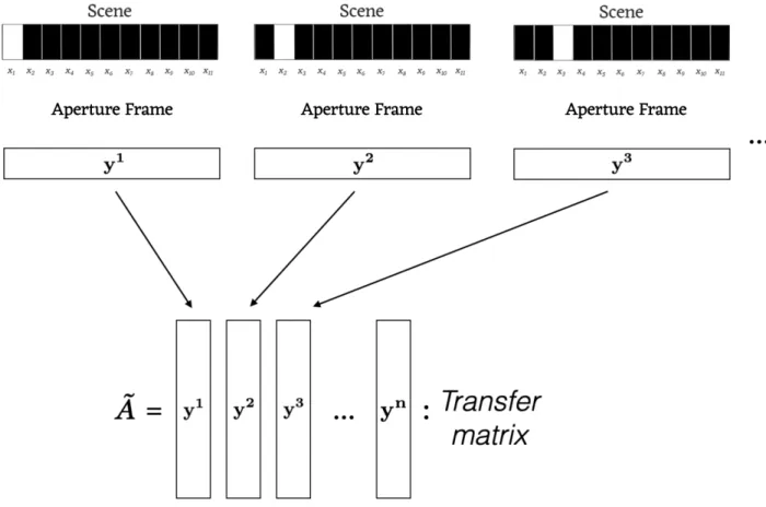
the resolution level being 𝑛 = 11. Note the labeling is reversed on the observation relative to the scene. The faithfulness of the modeled configuration to the true configuration will get better and better as 𝑛 increases. . . 50 1-9 How the transfer matrix comes out of the imaging system: each

col-umn of the transfer matrix corresponds to the illumination pattern on the observation plane in response to an impulse light source at each different point in the scene. . . 51 1-10 Three imaging systems (left column, top-to-bottom): no aperture, a

pinhole and a lens. Arrows indicate paths light from the scene takes to a particular point on the imaging plane. On the right is an arbitrary mask, an illustration of its discretization and the corresponding transfer matrix. . . 52

(16)

1-11 Top row: IID scenes with 𝜎 = 1, with three different levels of scene discretization (𝑛 = 50, 𝑛 = 200, and 𝑛 = 1000). Bottom row: each of those scenes, pixellated so that they have 50 pixels to a side. As you can see, the pixellated scenes look different from each other—this is a problem, because how finely we choose to discretize the scene shouldn’t make a difference to what the scene looks like. This is why IID scenes of different levels of discretization are qualitatively different from each other, unlike correlated scenes whose covariance matrices are chosen carefully to scale properly with discretization level. . . 55 1-12 Top row: Correlated 50 × 50 scenes with three different values of 𝛽.

𝛽 = 1 implies an IID scene, with increasing correlation as 𝛽 approaches 0. On bottom: the covariance matrix with 𝛽 = 10−5. Note that the covariance matrix is 2500 × 2500, since it describes the covariance of each of the 2500 scene pixels with each other pixel. The pattern of banding that you see depends on how we choose to flatten the 50 × 50 scene array into a 2500-entry vector; here, the scene is flattened in row-major order. . . 57

2-1 This figure is due to the authors of [67]. Top: A 2D light-field of a 1D scene. The horizontal axis indicates space in the scene, while the vertical axis indicates spatial movement along the sensor array. Bottom: the green arrows, inferred by the system of [67], point in the direction of the estimated disparity slope. Along them, the variance of the light-field is very small. This phenomenon is due to the fact that a light-field is simply the scene, seen from every possible sensor on the sensor array; as you move your vantage point along the sensor array, the scene will be nearly the same, except shifted. . . 63 2-2 A hexagonal grid, due to [55], which achieves spectral flatness, making

(17)

3-1 A once-repeating occluder, with its associated transfer matrix. As is apparent, the transfer matrix is circulant, with each row of the transfer matrix being a rotation of the pattern that is repeated once. See Figure 1-9 for a reminder on how the transfer matrix is created from an aperture frame. . . 74

3-2 These are the first few Paley sequences, i.e. on-off patterns whose spec-trum is flat and that yield a DMBC (determinant-maximizing binary circulant) when used as the first row of a circulant matrix. On the left is 𝑛, the number of on/off patches used. Note that for a Paley sequence to exist, 𝑛 must be prime and congruent to 3 mod 4. . . 80

3-3 Paley sequences, the “optimal” occluding masks that be constructed from them, and the transfer matrices associated with those masks. Left: we consider the Paley construction applied to the case 𝑛 = 11. The Paley construction gives us a binary sequence, with 1’s (white, or “on”) element 𝑖 of the sequence if 𝑖 is 0 or a quadratic residue modulo 𝑛, and 0’s (black, or “off”) for elements 𝑖 of the sequence if 𝑖 is not a quadratic residue modulo 𝑛. From this sequence we get an occluding mask, which consists of the sequence twice; every element is repeated exactly once except for the 0 element, which is in the center. Given the paraxial approximation and assuming the occluder is halfway in be-tween observation and scene, an impulse scene will cast a shadow that corresponds to half the occluder, which is some rotation of the original Paley sequence. Right: sequences given by the Paley construction (as well as any other flat sequence) are as different as possible from their own rotations; this means that depending on where the impulse light source is in the scene, the cast shadows will be as different as possible. This makes reconstructing the location of a point light source, given a cast shadow, as easy as possible. . . 81

(18)

3-4 Two plots of the ratio of the performance of various sequences to Hadamard’s upper bound, 𝑈01(𝑛) = 2−𝑛(𝑛 + 1)(𝑛+1)/2. The left plot

in-cludes the best possible binary matrix for each value of 𝑛 (note that the best possible binary matrix achieves Hadamard’s upper bound when a known construction for a DMBC exists, and not otherwise). The right plot extends the plot up to higher values of 𝑛, but can’t include the performance of the best possible binary matrix, because it takes too long to find for values of 𝑛 much greater than 50. . . 84

3-5 The number of satellites per local optimum, as estimated by sampling, including a line of best fit. This suggests approximately 1.22𝑛satellites per local optimum in the space of maximal determinants of binary sequences, implying a simple search algorithm should be able to find the global optimum in 𝑂(𝑛2_1.78𝑛_{) time. . . .} ₈₄

3-6 Left: the approximate effective pixels-per-side count of scenes gener-ated with a given level of correlation (𝛽) and under a given signal-to-noise ratio (SNR). 𝑛 = 1023. As expected, more correlated scenes and noisier scenes both have fewer effective pixels. Note, however, that even highly correlated scenes can have high effective pixel counts if the SNR is high enough, but if the SNR is low enough the scene will always have a low effective pixel count. Effective pixel count was estimated by choosing which of the nine spectrally-flat masks shown on bottom yielded the highest mutual information. Right: masks corresponding to each of the effective scene pixel counts. Note that these masks repeat themselves once in each dimension, so each mask is 2𝑛 − 1 × 2𝑛 − 1 if the effective pixel count is 𝑛. This is due to the phenomenon described in Figure 3-3. . . 86

(19)

3-7 Top left: the approximate effective pixels-per-side count of scenes gen-erated with a given level of correlation (𝛽) and under a given signal-to-noise ratio (SNR). Alternately, the plot shows which of the masks shown in the top right is optimal, assuming you are forced to choose one of those four. Top right: masks corresponding to each of the ef-fective scene pixel counts. Bottom: the difference between the MI performance of the best mask from among the four masks in the top right and the best possible mask, as a percentage of the MI perfor-mance of the best possible mask, as found by exhaustive search. Thus for 𝑛 = 15, choosing your mask from only the four masks in the upper right is no more than 0.2% worse than using the very best mask. . . . 88

3-8 Top left: the approximate effective pixels-per-side count of scenes gen-erated with a given level of correlation (𝛽) and under a given signal-to-noise ratio (SNR). Alternately, the plot shows which of the masks shown in the top right is optimal, assuming you are forced to choose one of those four. Top right: masks corresponding to each of the ef-fective scene pixel counts. Bottom: the difference between the MI performance of the best mask from among the seven masks in the top right and the best mask found with a greedy search, as a percentage of the best mask from among the seven masks in the top right. Positive percentages mean that choosing the best mask from a menu is better; negative percentages mean that a greedy search is better. We can see that choosing from a menu of URAs at different scales outperforms greedy search in the high-SNR regime, and does worst at the boundary between masks at different scales, which is intuitive. . . 89

3-9 Reconstructions of a simulated scene with (lower-right) and without (lower-left) a prior. . . 90

(20)

3-10 The probability density function 𝑓𝑋(𝑥) = |𝑥|𝑒−𝑥

2

, which characterizes the probability of getting an eigenvalue of each possible magnitude for a circulant matrix whose entries are IID with mean 0, variance 1, and bounded third moment. As 𝑛 → ∞, this plot will look just like a histogram of such a matrix’s eigenvalue magnitudes. . . 96

3-11 A plot of optimal transmissivity parameter 𝑝⋆ for random on-off pat-terns in the IID scene model, as we vary shot noise power 𝐽 and signal strength 𝜃 while ambient noise power 𝑊 is held fixed. See Remark 1. 98

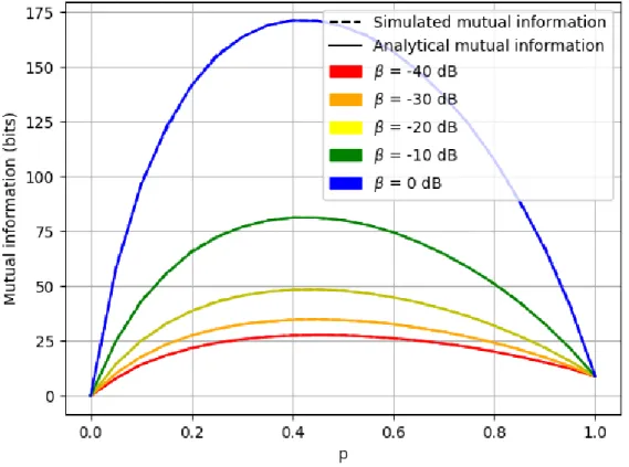
3-12 Analytical formula follows Eqn. (3.23). Simulated data are averages of 200 randomly generated apertures of size 𝑛 = 251 for various different values 𝑝. We set 𝐽/𝑊 = 0 dB and 𝜃/𝑊 = 30 dB. Simulations match our analysis perfectly, providing support for the conjecture of (3.23). 103

3-13 In this figure we plot the mutual information of a random on-off mask as a function of 𝑝. In blue is the simulated mutual information, obtained by generating 100 random sample masks and averaging. In red is the mutual information implied by Proposition 3.7.4. For both curves, 𝑚 = 𝑛 = 1000. The point here is we have some evidence for the truth of the conjecture we made right above Equation 3.23. . . 104

3-14 Two simulated reconstructions of a scene, using a random occluder (left) and a spectrally-flat occluder (right). The SNR is 10dB. Recon-structions are performed using the procedure described in Section 3.6, using an exponential-decay prior with 𝛽 = 0.1. As can be seen, using a spectrally-flat occluder results in substantially higher reconstruction quality. . . 106

(21)

3-15 Two simulated reconstructions of a scene, using a pinhole (left) and a spectrally-flat occluder (right). The SNR is 10dB. Reconstructions are performed using the procedure described in Section 3.6, using an exponential-decay prior with 𝛽 = 0.1. As can be seen, using a spectrally-flat occluder results in substantially higher reconstruction quality. Note that the observation using a pinhole is much more in-telligible than that obtained using a spectrally-flat occluder, but this does not translate to higher reconstruction quality. . . 107 3-16 Three spectrally-flat sequences with transmissivities not equal to 1/2. 110 3-17 A pair of scatter plots comparing the LMMSE-minimizing metric to

the MI-maximizing one. In each case, we have 𝑡 = 1, 𝑊 = 1, 𝐽 = 0, 𝜃 = 100. In the left plot, we have one point for every 11 × 11 binary circulant transfer matrix; in the right, we have one plot for each of 1000 randomly-chosen 100 × 100 binary circulant transfer matrices. . 111 3-18 A side-by-side comparison of reconstructions of the same scene

un-der the same conditions, but using two different occluun-ders: one (left) preferred by the MSE-minimizing metric, the other (right) by the MI-maximizing metric. As expected, the MSE of the right reconstruction is worse, but the image appears to be somewhat sharper. . . 112 3-19 A simple layout that explains the phenomenon whereby the relative

speeds of a light source and its shadow are given by the relative dis-tances of the scene and the observation to the occluder. Suppose we have a pinspeck occluder, and a light source that moves by an amount ∆1 to the right. If we suppose that its shadow moves by an amount

∆2 to the left, and that the occluder has a perpendicular distance 𝑑1

from the scene and 𝑑2 from the observation, then the fact that the top

and bottom triangles are similar tells us that ∆1/∆2 = 𝑑1/𝑑2. . . 114

3-20 Top row: five different scenarios with the occluder at five different depths. Bottom row: the transfer matrices corresponding to each dif-ferent scenario. . . 116

(22)

3-21 Top: a configuration with a planar occluder not halfway in between the scene and the observation. If we take the distance between the scene and observation to be 𝑑, then the distance between the scene and occluder is ₂₂9 𝑑 and the distance between the occluder and observation is 13₂₂𝑑. We take a discretization level of 𝑛 = 11 (so for computational reasons, we are modeling the scene and observation as vectors of 𝑛 = 11 constant entries, and the occluder as a vector of 2𝑛 − 1 = 21 constant entries). Bottom left: the true, continuous transfer matrix. Bottom middle: the naive discrete 11×11 approximation of the transfer matrix, using averaging to produce nonbinary elements. Bottom right: the “stretched” 9 × 13 approximation of the transfer matrix, yielding a rectangular matrix with Toeplitz structure and only binary elements. 118

3-22 A comparison of observed mutual information using either a square matrix with non-binary averaged values, or a stretched rectangular matrix, appropriately rescaled. In this example, 𝑛 = 61. It is apparent that the effect of averaging values in the square matrix leads to a dra-matic (and artifactual) decrease in the observed mutual information, as well as artifacts at depths that make there be fewer nonbinary values in the square matrix. . . 120

3-23 Top: the approximate effective pixel count of scenes generated at dif-ferent occluder depths. As expected, when the occluder is near the ob-servation plane or the scene, it reduces the number of effective pixels. Here the frequency attenuation coefficient 𝛽 = 0.1. Higher values of 𝛽 correspond to less correlated scenes. Bottom: masks corresponding to each of the effective scene pixel counts. Note that these masks repeat themselves once in each dimension, so each mask is 2𝑛 − 1 × 2𝑛 − 1 if the effective pixel count is 𝑛. This is due to the phenomenon described in Figure 3-23. . . 122

(23)

3-24 Left: the transfer matrix from a pinhole. Right: the transfer ma-trix from very strong near-field effects (𝑑 = 0.01𝑥, where 𝑑 and 𝑥 are the distance from scene to observation and size of observation, respec-tively). As can be seen, the transfer matrices look identical but for a vertical (or horizontal) reflection. . . 124 3-25 Left: the transfer matrix from an occluder-based imaging configuration

with strong near-field effects. Right: the imaging configuration. . . . 125 3-26 A resolution plot showing the effective pixels per side as a function of

the SNR and the distance of the scene from the observation. 𝛽 = 0.1. The length of 𝑥max of the observation and scene is 𝑥max= 1. . . 125

3-27 Left: a traditional pinhole of size 𝑟 = 0.1, and its associated transfer matrix. Right: a circulant pinhole of size 𝑟 = 0.2, and its associ-ated transfer matrix. Note that the transfer matrix on the left is not circulant, but the one on the right is. . . 127 3-28 Optimal (circulant) pinhole size, as a function of scene correlation and

SNR. Note that optimal pinhole size depends primarily on SNR, and only secondarily on scene correlation. . . 130 3-29 If you could perfectly reconstruct a light field using an occluder (the

chair, outlined in blue) the reconstruction would be what can be seen on the right of this figure: the scene, as seen from every point (in green) on the observation plane (outlined in red). . . 135 3-30 Top: the configuration of the imaging system. The scene is made up

of two opaque frames, one red and one blue, at 𝑧 = 8 and 𝑧 = 11, respectively. Bottom: the light-field corresponding to that configura-tion (i.e. the appearance of the scene, viewed from every point on the observation plane). . . 138

(24)

3-31 Top: the estimated non-self-occluding 3D space, using a least-squares method. Bottom: the light-field derived from that space. As can be seen, despite the fact that the 3D space estimate is a terrible estiamte of the true 3D space, the light-field that results is very close to the true light-field. . . 139 3-32 Top: the scene configuration. Note that we are using the paraxial

approximation, so the width of the scene and observation plane are taken to be much smaller than the scale of this figure would suggest. The optimal occluder (found by exhaustive search over all 210_occlusion

possibilities in the 2 × 5 grid shown in grey) is not planar. The scene is IID, 𝜎 = 103_{, 𝑘 = 10, 𝑛 = 100. Bottom: the 𝑛 × 𝑘𝑛 transfer matrix}

corresponding to the occluder shown above. . . 140 3-33 Top: the scene configuration. Note that we are using the paraxial

ap-proximation, so the width of the scene and observation plane are taken to be much smaller than the scale of this figure would suggest. The locally optimal occluder (found by greedy search over the 236occlusion possibilities in the 4 × 9 grid shown in grey) is not planar. The scene is IID, 𝜎 = 103, 𝑘 = 10, 𝑛 = 99. Bottom: the 𝑛 × 𝑘𝑛 transfer matrix corresponding to the occluder shown above. . . 141 3-34 An example scene flattened using row-major order, and an example 2D

occluder’s corresponding convolutional transfer matrix. Note that the transfer matrix is “2D-Toeplitz” without being Toeplitz in the ordinary sense. This means that it will be near-diagonalized by the flattened 2D Fourier basis (rather than the 1D Fourier basis). . . 145 3-35 This section’s definition of tensor-matrix multiplication, with a worked

example. . . 147 3-36 A circulant (3 × 3) × (3 × 3) tensor. . . 147

(25)

3-37 Top: a flatland configuration with an edge occluder. Bottom left: the transfer matrix corresponding to this occluder. Bottom right: the inverse of that transfer matrix. The transfer matrix 𝐴 corresponds to spatial integration, and its inverse 𝐴−1 to spatial differentiation. . . 148 3-38 Top: two imaging configurations near a doorway; the two different

scenes lead to two different light reflections on the ceiling. Note that the observation on the ceiling is equal to the scene, integrated along both spatial dimensions. Bottom: the inversion process for this occluder. Because this occluder is separable, it suffices to do two operations, one along one of the dimensions, and one along the other. . . 150 3-39 A (2 × 2) × (2 × 2) separable transfer tensor 𝒜 (in black). Each of its

submatrices can be expressed as an outer product of vectors 𝑢𝑖 (blue)

and 𝑣𝑖 (red), each of which make up the matrices 𝑈 and 𝑉 respectively.

For all 2 × 2 matrices 𝑋, we will have 𝒜𝑋 = 𝑈 𝑋𝑉𝑇_. _{. . . .} ₁₅₂

3-40 A simulated scene, transformed by two equivalent occluders, 𝐴1 and

𝐴2. Despite the fact that the two potential observations 𝑌1 and 𝑌2

you would get by transforming the scene 𝑋 by each of 𝐴1 and 𝐴2

look nothing alike, the reconstruction you get by computing 𝐴−1₂ 𝑌1 is

almost identical to the scene. This is useful, because 𝐴2 is a separable

occluder and 𝐴1 is not. . . 154

3-41 An experiment with a right-angle occluder (the stack of legos) where one quadrant occludes and the other three do not. This occluder is not separable, but it is equivalent to one that is. The ground truth image was displayed on a monitor to yield the observation. Thus the reconstruction can be obtained simply by taking the derivative of the cropped observation along both spatial dimensions. Note that when using a prior, this causes large, ugly artifacts to appear, especially near the edge of the image. . . 156

(26)

3-42 Another family of equivalent occluders. Any of these occluders can be freely substituted for any of the others, and most of the pixels of the resulting image will be exactly correct. . . 157 3-43 Left: a configuration with an edge occluder parallel to the scene. To

get a 1D reconstruction of the scene, we sum the intensities along the 𝑦 dimension and differentiate along the 𝑥 dimension. Right: a configuration with an edge occluder perpendicular to the scene. To get a 1D reconstruction of the scene, we sum the intensities along the 𝑟 dimension and differentiate along the 𝜃 dimension. . . 157 3-44 A woman holding a flashlight above a book with one hand, and holding

a book above the table with the other, as described in the third para-graph of Section 3.20. If she moves the flashlight around, it will move the shadow edges 𝑢 and 𝑣, but 𝑢 and 𝑣, if extended, will always go through 𝑝𝑢 and 𝑝𝑣, the focal points of this occluder, no matter where

the flashlight may be. The focal points 𝑝𝑢 and 𝑝𝑣 can be found by

ex-tending the edges of the book downward until they intersect the table. 𝑝𝑣 (in green) is to the right of the frame; it would appear when the

green dotted line intersected the table. . . 159 3-45 The transformation from locations on the observation plane to points

in the scene, for a given pair of focal points. . . 160 3-46 Left: A Fresnel lens. Right: A convex lens of equivalent power. Note

that the thickness of the glass at each point on the Fresnel lens is equal to that of the convex lens, modulo the maximum thickness of the Fresnel lens. Image credit due to Wikipedia. . . 162 3-47 The displacement 𝑑 of an incoming light ray increases with the

(27)

3-48 Top: the performances of optimal transmissive aperture frames for three different choices of 𝑛2 (corresponding to the approximate

refrac-tive index of glass, diamond, and silicon, respecrefrac-tively), and for three different choices of the glass’s thickness. Unsurprisingly, optimal per-formance improves with higher thickness and higher refractive index. Other parameter choices are 𝑛 = 8, 𝑥 = 1, 𝑦 = 1, the SNR 𝜎 = 103_,

and the scene correlation coefficient 𝛽 = 0.1. Each sub-image shows the form of the aperture frame on the left, and the corresponding trans-fer matrix on the right. Bottom: for comparison, the performance of the optimal occluding aperture frame, under identical conditions. As can be seen, using an occluder substantially outperforms all but the thickest glass, if the glass is assumed to be flat. . . 165

4-1 A method for constructing a 1-D video of an obscured scene. The far left shows a diagram of a typical scenario: two people—one wearing red and the other blue—are hidden from view by a wall. To an observer walking around the occluding edge (along the magenta arrow), light from different parts of the hidden scene becomes visible at different angles (A). Ultimately, this scene information is captured in the inten-sity and color of light reflected from the corresponding patch of ground near the corner. Although these subtle irradiance variations are invis-ible to the naked eye (B), they can be extracted and interpreted from a camera position from which the entire obscured scene is hidden from view. Image (C) visualizes these subtle variations in the highlighted corner region. We use temporal frames of these radiance variations on the ground to construct a 1-D video of motion evolution in the hidden scene. Specifically, (D) shows the trajectories over time of hidden red and blue subjects illuminated by a diffuse light in an otherwise dark room. Figure originally from [16]. . . 168

(28)

4-2 Left: the percent difference in performance between the edge camera and optimal size of circulant pinhole for each value of SNR and 𝛽. Negative values indicate that the pinhole outperforms the edge camera. Right: the percent difference in performance between the edge camera and a circulant pinhole camera with transmissivity 𝜌 = 1/4. . . 169 4-3 Top left: an idealized setting in which scene, observation, and occluder

are all parallel. Bottom left: a simplified version of the setting in flat-land, in which the region highlighted in cyan in the top left is averaged to produce the region highlighted in cyan in the bottom left. Top right: the real-world setting in which the occluder lies perpendicular to the observation. Bottom right: a simplified version of the setting in flatland, in which the region highlighted in cyan in the top right is averaged to produce the region highlighted in cyan in the bottom right. 171 4-4 The example estimation gain image, showing the operation performed

on the observation to recover the scene. As we can see, it’s approxi-mately a spatial derivative along the angular dimension. The spatial derivative being taken has a “blurry” appearance because of the spatial prior. Figure originally from [16]. . . 174 4-5 Indoor experiments for the corner camera. The subjects’ trajectories

are clear from the traces in the reconstructed 1D movie (right). Note that the 𝑥-axis corresponds to time. Note, also, that the number of subjects can be easily counted.Figure originally from [16]. . . 175 4-6 Outdoor experiments for the corner camera. In sunny weather, the

subjects’ trajectories are very clear. In cloudy weather, the trajectories are fainter but still clear upon closer examination. In rainy weather, the raindrops create dark streaks in the reconstructed movie trace. However, if we ignore those streaks, we can still see most of the subjects’ trajectories.Figure originally from [16]. . . 175

(29)

4-7 This figure shows the configuration for the toy problem of interest. The scene consists of a single bright object, whose angular position 𝜃 we want to learn. . . 177 4-8 This figure shows the impact of a corner location error. In the

error-free case, we would sweep 𝜑 across the projection plane (shown in green) hinging around the corner (the solid black line). But if we made a corner location error, we would instead try to sweep 𝜑 across the projection plane erroneously (shown in blue) hinging around the false corner (shown with a dotted line). . . 178 4-9 This plot shows how the observed intensity values vary with 𝜑, in the

case of correct corner location (in blue) and a corner location error ((𝑑𝑥, 𝑑𝑦) = (0.1, 0.2), in red). Note that in the case of a corner location

error, the maximum value of the intensity does not reach 1. Note also that 𝑑𝑥 and 𝑑𝑦 are as a fraction of the radius of the projection plane,

𝑟, which here is taken to be 1. . . 179 4-10 This plot is intended as a reference for the meanings of each of the

variables used in the calculations of 𝜑 as a function of 𝜃. . . 180 4-11 This plot shows the empirical mean (in blue) plus or minus one

stan-dard deviation (in red) of the error as a function of 𝜃. Here, 𝜎𝑥 = 10−4

and 𝜎𝑦 = 10−3. . . 181

4-12 The empirical means plus or minus one standard deviation of the esti-mated 𝑃𝑧 as a function of its 𝑥-coordinate, assuming true 𝑃𝑧 of 20, 40,

60, and 80. Here, the two corner location errors at each of the bound-aries of the doorway are independent and subject to 𝜎2_Δ𝑥= 𝜎2_Δ𝑧 = 0.04. We sample from a set of 1000 corner errors to approximate the mean and standard deviations empirically. . . 182 4-13 The reconstructed depths of objects at depths 1, 2, 3, and 4, given a

(30)

4-14 The reconstructed depths of objects at depths 1, 2, 3, and 4, given a corner error of ∆𝑦1 = −0.02, ∆𝑦2 = 0.02. Note that because of

the different corner errors for each corner, there is the possibility of asymmetric behavior on either side of the doorway. . . 184 4-15 The process of calibrating for the occluder, performed by lighting one

small region of the monitor on the left at a time, and recording the shadow on the right that results. Note the similarity of this process to the definition of the transfer matrix from Chapter 1. . . 186 4-16 a) Simplified 2D scenario, depicting all the elements of the scene

(oc-cluder, hidden scene and observation plane) and the parametrization planes for the light field (dashed lines). (b) Discretized version of the scenario, with the light field and the observation encoded as the dis-crete vectors x and y, respectively. The transfer matrix is a sparse, row-deficient matrix that encodes the occlusion and reflection in the system. . . 187 4-17 a) Sketch of a 2D imaging scenario. (b) Resulting unoccluded light

field function 𝑙(𝑥, 𝑢) and observation. (c) The occluder visibility func-tion 𝑣(𝑥, 𝑢). (d) Resulting occluded light field funcfunc-tion 𝑙𝑜𝑐𝑐(𝑥, 𝑢) =

𝑣(𝑥, 𝑢)𝑙(𝑥, 𝑢) and observation. Note that the unoccluded observation is almost constant in 𝑢, which is not true of the occluded observation; the presence of the occluder makes the problem better-conditioned. Figure originally from [12]. . . 188 4-18 Reconstructions of an experimental scene with two rectangles. (a)

Schematic of the setup. (b) Observation plane after background sub-traction. (c) Six views of the true scene, shown in order to demonstrate what the true light field would look like. These are taken with a stan-dard camera from equivalent positions on the observation wall. (d) Reconstructions of the light field for these views. The blue and red targets measure 8 × 12in and 6 × 8in. Figure originally from [12]. . . 189

(31)

4-19 Reconstructions of an experimental scene with a seated subject at the scene plane. (a) Observation plane after background subtraction. (b) Six views of the true scene.(c) Reconstructions of the light field for the same views as in (b). Figure originally from [12]. . . 190 4-20 Left: a real-world scenario with a moving scene, an occluder, and an

observation wall. Right: our model of the scenario. . . 191 4-21 A worked example of initialization of Algorithm 1, followed by a single

pass through the for-loop. Continued in Fig. 4-22. . . 197 4-22 A worked example of Algorithm 1. . . 198 4-23 An illustration of the effects of the planarity assumption and the

parax-ial approximation on the reconstruction. The top row shows a sketch of the true setup; in all three cases, the assumed setup is the one on the left. The middle row shows what reconstructions, generated using the approach described in Sec 4.5.7, of the leftmost image look like when the assumptions used for that approach are violated. The bottom row shows example impulse responses for each of the three scenarios. All data shown here is simulated, with no noise, to isolate the effect of each assumption. . . 203 4-24 The output of the occluder-recovery and scene-reconstruction

algo-rithms presented in Secs. 4.5.3 and 4.5.7, using the difference frames of a simulated observation at 25dB. . . 204 4-25 The output of the occluder-recovery algorithm presented in Section 4.5.3

in the experimental setting, alongside the ground-truth occluder. This is the occluder recovery used in the reconstruction shown in the second row of Figure 4-26. . . 206

(32)

4-26 Still frames from reconstructed videos under a variety of different ex-perimental settings. Top row: the scene is a cartoon video, playing on an LCD monitor. Middle row: the scene is a moving man, illumi-nated by 200W of directed lighting. Bottom: the results of Saunders et al. [86], presented for comparison. The results of Saunders et al. demonstrate the potential improvement over our result when the form of the occluder is known. See Subsec. 4.5.14 for further discussion. . . 207

4-27 Blind light transport factorization using the method of [6]. The first three sequences are projected onto a wall behind the camera. The Lego sequence is performed live in front of the illuminated wall. Figure originally from [6]. . . 213

5-1 Left: an 10𝜇𝑚 IR image of a faint reflection of a human hand, reflected by marble that appears matte in visible light. Lighter colors correspond to higher intensities. Right: a speculative depiction of the surface of the marble. Because it appears matte in visible light but is specular in IR, we can infer that it is likely jagged on a scale between 700𝑛𝑚 and 10𝜇𝑚. . . 218

5-2 A reprint of Figure 3-7, assuming a 2𝑚 scene and observation. The dark rectangle indicates a range of realistic experimental settings for a 2D passive occluder-based reconstruction. As shown above, even with the ideal occluder, resolution on a scale of centimeters is very difficult to achieve. . . 221

(33)

5-3 Top: The unscrambling results using each of four different dimension-ality reduction algorithms for a short (624-frame) video, scrambled uniformly at random, with the best results achieved by Isomap, fol-lowed by Locally Linear Embedding. Bottom: A comparison of a re-constructed (unscrambled) frame with a ground-truth frame from the original video, using a Voronoi mapping of colors to locations in the unscrambled video. As can be seen, the reconstruction is quite good, except at the edges of the frame where the scale is wrong. . . 224 5-4 We can use dimensionality-reduction techniques and the ball-tree data

structure to reconstruct a 3000-frame video seen through a water bot-tle. Shown is a single frame of the reconstructed video. Note that because of fundamental ambiguities, the reconstructed frame is a rota-tion and reflecrota-tion of the ground-truth frame. . . 225 5-5 A possible observation plane that could make use of parallax from

multiple 1D occluders. Each of the signpoles near the road act as 1D pinspeck occluders, but light sources in the street will cause them to cast shadows that extend in different directions, creating a potentially useful parallax effect. . . 227

(34)

(35)

Chapter 1 Introduction

What is a camera? The dictionary tells us that a camera is an “optical instrument to record images.” When you think of a camera, you probably think of something with a lens, like a digital camera or, more recently, a smartphone—or, in the future, perhaps something else entirely. Lenses are very effective imaging tools—indeed, even our eyes evolved to use them!—but cameras can be built without them. The first known camera that could create permanent photographs was developed by Joseph Nicéphore Niépce, who used a camera obscura, or pinhole camera, to project an image of a scene onto dark pewter coated with bright bitumen [44]. The bitumen, exposed to light, hardened and became insoluble, so that it would not wash off the pewter when rinsed with water, leaving the parts exposed to the light to stay white while the rest turned dark. See Figure 1-1 to see the earliest surviving photograph.

This photograph was created by a pinhole camera, which is part of a class of cameras that I call “occluder-based” cameras. An occluder is any object that blocks light; in the case of a pinhole camera, this object blocks nearly all of the light, except for that which is allowed to pass through a tiny hole. Pinhole cameras are special, because the image projected onto the pewter is identical to the scene, except that it’s spatially reversed and blurred in proportion to the size of the hole. That makes the design of a pinhole camera the simplest of the occluder-based cameras, because the projected image is easily interpreted, without any need for further computation. Simplest, however, does not mean best, and more recently-developed occluder-based

(36)

Figure 1-1: The earliest surviving photograph, taken by Joseph Nicéphore Niépce in 1825, using an occluder-based camera.

(37)

cameras [9, 30, 102, 41] have abandoned the pinhole in favor of more complicated patterns of occlusion. These more complicated patterns vary from implementation to implementation, though the most popular choice is a set of patterns called “uniformly redundant arrays.” Each of these non-pinhole patterns yield unintelligible projected images, but enable much more accurate computational reconstructions in the presence of noise. See Figure 1-2 for a side-by-side simulated comparison of the two methods. One of the contributions of this thesis is provide a framework, based on information theory, that explains why uniformly redundant arrays are better than pinholes. Using this framework, I will describe the circumstances under which we know uniformly redundant arrays are the best option, and how to choose which uniformly redundant array to choose. This is what Chapter 3 is about: choosing the best occluder-based camera system possible, given a particular set of imaging circumstances. Occluder-based designer cameras aren’t the only topic of this thesis, however. In addition to designer cameras, this thesis contributes to the field of occluder-based accidental cameras.

Before I explain the concept of accidental cameras, let’s revisit the question we began with. What is a camera? A camera is an optical instrument to record images. What are cameras made of? Generally, cameras are the combination of two objects. The first is what I will eventually call the “observation plane,” or more simply the “observation.” This object is generally something photosensitive, like film, a digital light sensor, or pewter coated with bitumen as in our earlier example. The second is what I will eventually call the “aperture frame.” The purpose of this latter object is simply to make the observation non-uniform. It’s necessary to have something in between the scene and the observation, be it a lens or an occluder, because without it, our observation would be uniformly illuminated. This, in turn, means the observation would contain almost no information about the scene.

Accidental occluder-based cameras take a creative approach to both the obser-vation and the aperture frame. In most of the accidental-camera systems described in this thesis, the observation plane is a blank wall or floor, recorded by a digital camera positioned elsewhere (the “observer”). The aperture frame is some occluding

(38)

Figure 1-2: This figure will appear again, later in this thesis, when more context with which to understand it has been given. The point here is that when the simulated unknown scene (top middle) is projected through a pinhole occluder (top left), it results in a more intelligible projected image, or “observation” (middle left) but a lower-quality reconstruction of the scene (lower left). In constrast, when the simulated unknown scene is projected through a more complicated occluder, in this case a uniformly redundant array (top right), it results in a less intelligible projected image (middle right) but a higher-quality reconstruction of the scene (lower right). It makes sense that historically, the simpler (left) approach would be the first, because no computation is required to understand the observation, but the more sophisticated (right) approach is more powerful.

(39)

object, like a wall (see Section 4.1) or any opaque object (see Section 4.3 or 4.5). One possible purpose of an accidental occluder-based camera is non-line-of-sight (NLoS) imaging: in other words, to “see” things are not directly in view of the observer. To give a very basic example, imagine you are sitting in your room, with sunlight shining in from a window. From the square of sunlight on the floor, and the location of your window, you can infer in what direction the Sun is. In a certain sense, you have “seen” the Sun; without actually looking out your window, you know where it appears in the sky. Even if you don’t know exactly what you would see if you looked out your window, you know where the Sun would be in that picture.

The same method that you used to infer the position of the Sun without looking out your window, could in principle be used to infer the position of everything else visible from your window, without looking out your window. This is because it’s not just the Sun that emits light; visible objects are visible because they emit (reflected) light, it’s just that they are emitting much less light. But even if it’s too subtle to be seen with the naked eye, there is light streaming through your window that comes not directly from the Sun, but reflected off something outside, and if you were sharp-eyed enough to see it, you would be able to infer exactly what was outside your window, without actually looking out your window. Indeed, this is more or less exactly what was shown by Torralba and Freeman in 2012 [97], in one of the first publications to discuss occluder-based accidental cameras.

What good is it to use sophisticated computational techniques to infer what you would see if you were to look out a window? Why not just look out the window, like a normal person? There are scenarios in which being able to solve analogous problems can be very useful. For example, this style of imaging technique could let you “see” into a room you didn’t want to enter (see Figure 1-3). Perhaps even more usefully, occluder-based accidental cameras could be used to detect oncoming traffic around a corner, and help prevent life-threatening collisions (see Figure 1-4). Additionally, occluder-based systems can be used to create smaller cameras than lenses allow [9] or to perform X-ray imaging, which is often incompatible with lenses [1].

(40)

Figure 1-3: A hypothetical scenario in which occluder-based techniques could be used for non-line-of-sight imaging. On the left, we can see a door, but we don’t know anything about what’s in the room it leads to (shown on the right). Together, the door and the chair inside the room form an accidental camera. Using the method presented in Section 4.5, an onlooker could, in principle, try to reconstruct an image of the room by observing the door by using the occlusion provided by the chair and the motion provided by the person. This is true even though neither the chair nor the person is visible to the onlooker! I say “in principle” because in practice, the signal strength in the room as shown would be too weak to get a sharp reconstruction— this is meant as an illustration of what is possible with accidental cameras, not a description of current capabilities.

(41)

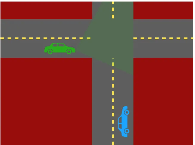
Figure 1-4: Imagine you are in the blue car, approaching the intersection ahead. There’s a green car headed towards the intersection around the corner, but you can’t see it, because there’s a building blocking your view. However, the green car is reflecting green light onto the street in front of you, and that green light is something that is within your field of view, even if it’s too faint to be seen with the naked eye. The intersection in front of you, combined with the building to your left, form an accidental camera. An automatic driving system could use it to infer the angle from the corner and the speed of the green car around the corner using the computational imaging techniques described in Section 4.1. Systems like these could be used to avoid a deadly collision, if the green car is about to run a red light.

(42)

The contents of Chapter 3 (which is broadly about finding the best possible occluder-based aperture frame) and those of Chapter 4 (which is about making use of whichever occluders happen to be handy in NLoS settings) are largely separate. However, the analysis of Chapter 3 is of obvious relevance to NLoS occluder-based imaging even when finding an optimal occluder “in the wild” isn’t realistic.

The framework described and used in this thesis is a powerful tool for analyzing occluder-based imaging. Occluder-based non-line-of-sight imaging remains a promis-ing area for future research, with the deep image prior bepromis-ing particularly promispromis-ing, as discussed in Section 4.6.

1.1 Overview

This thesis is meant to serve a few purposes simultaneously. The first will be to provide a clear and easy introduction to the core concepts of occluder-based imaging; my hope is that anybody who wishes to learn more about the topic, either because they are interested in an application in non-line-of-sight imaging purposes, coded-aperture imaging, or some other application, will find this thesis to be helpful. I am also hopeful that this thesis can be understood even by readers with relatively little background; I intend for many of its sections to be comprehensible without any background in physics or optics, and only an undergraduate-level understanding of linear algebra, signal processing, and calculus (in decreasing order of importance).

Chapter 3 gives a complete treatment of which mask-based occluders are optimal, under a variety of different scenarios, as well as a novel framework for analyzing mask-based occluders. When optimality can’t be proven, Chapter 3 is still able to give specific, helpful advice for which mask-based occluders are likely to perform best. The contents of Chapter 3 will be helpful for designing an occluding-mask-based camera. For other types of nontraditional cameras—cameras that use a different sort of aperture frame, perhaps, but still not a lens (one example is the DiffuserCam [8])— extending the analysis of Chapter 3 should prove straightforward.

(43)

fo-cus is in non-line-of-sight imaging, especially passive non-line-of-sight imaging. Chap-ter 4 describes how to solve non-line-of-sight imaging problems under a variety of constraints.

1.2 Ray Optics and BRDFs

Throughout my thesis, unless I say otherwise, I’ll be using the ray optics model (also known as the geometrical optics model) of light. This means that, as a convenient abstraction, I’ll be assuming that light moves in a straight line through the air, can be bent when it hits a different light-propagating medium (like a lens), and may be absorbed or reflected by the materials it hits (like a wall). Moreover, I’ll be generally assuming that light intensity is additive, meaning that two rays of light hitting the same point will generate an intensity equal to the intensity that would be generated by the sum of each individual ray. This corresponds to assuming that the light we care about is incoherent and as such won’t interfere with itself—a reasonable assumption when the light in question is coming from the sun or from a commercial electric light. Finally, using the ray optics model means that I’ll be ignoring the effects of diffraction, which is reasonable when modeling the behavior of visible-wavelength incoherent light hitting macroscopic structures.

What happens when the light hits an opaque surface, according to this model? Some of it will be absorbed, and some reflected. How much of it is reflected, and in what directions, is described by the bidirectional reflectance distribution function, or BRDF, of the surface. In flatland (meaning a 2D world), the BRDF is a function of two variables, the angle of the incoming light 𝜔𝑖 and the angle of the outgoing light

𝜔𝑟, and returns the ratio of the reflected radiance (the outgoing power per unit angle

per unit projected area on the surface) along 𝜔𝑟to the irradiance (the incoming power

per unit area) incident on the surface from 𝜔𝑖.

There are a variety of BRDFs that describe real-world surfaces, including the specular BRDF (which describe mirrors and other shiny surfaces well) and Phong BRDFs (due to [80], which describe glossy surfaces well). In this thesis, however, the

(44)

focus is on the Lambertian BRDF, which is defined below: 𝑓Lambertian(𝜃in, 𝜃out) = 𝜌/𝜋

Surfaces that have this BRDF are often called Lambertian, matte, or diffuse sur-faces, and I will use these terms interchangeably in this thesis. Intuitively, this BRDF takes the incoming light and emits it “equally in all directions.” Once again 𝜌 is a constant that determines the overall surface brightess. Note that the Lambertian BRDF is completely independent of the angle of the incident light—it emits the light it reflects in exactly the same way no matter where the light came from.1

1.3 The Paraxial Approximation

In this section, I introduce the paraxial approximation, a commonly used assumption in computational imaging [109, 69, 94, 87, 25]. The idea is that when a light source is far from a surface, its illumination of that surface will be approximately uniform.

1.3.1 A point light source and a nearby surface

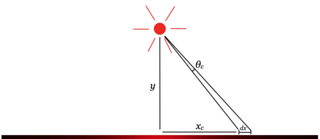
Let’s suppose we live in a 2D world of Lambertian surfaces and diffuse light sources. (When I say a “diffuse” light source, I mean that the light source emits light equally in all directions.) Consider a point light source suspended at (0, 𝑦𝑝), with a Lambertian

surface at 𝑦 = 0 (see Figure 1-5). What pattern of illumination can we expect to see on the surface?

The way we proceed with this analysis is to discretize the surface into many small patches, and then to consider what fraction of the light radiating out of the point light source hits any single given small patch of the surface. We assume each patch is small enough that its apparent intensity is constant across the patch. Asking what fraction of light radiating out of the point light source hitting any given patch is

1_{For a 2D surface living in a 3D world, the Lambertian surface BRDF is exactly the same, but}

(45)

Figure 1-5: A diagram illustrating the following configuration: a point light source at (0, 𝑦𝑝), with a Lambertian surface at 𝑦 = 0. We are interested in the resulting

illumination pattern on the Lambertian surface; to investigate it, we measure the illumination of a small patch on the surface that extends from (𝑥𝑐, 0) to (𝑥𝑐+ 𝑑𝑥, 0).

The illumination of that patch will be proportional to the angle 𝜃𝑐of the point source’s

light subtended by the patch.

equivalent to asking what angle over the light source is subtended by that patch, and then dividing that angle by 2𝜋.

Supposing that the patch extends from (𝑥𝑐, 0) to (𝑥𝑐+ 𝑑𝑥, 0), trigonometry tells

us that 𝜃𝑐, the angle subtended by the patch, is given by:

𝜃𝑐 = tan−1 (︂ 𝑥𝑐+ 𝑑𝑥 𝑦𝑝 )︂ − tan−1(︂ 𝑥𝑐 𝑦𝑝 )︂

What happens as we consider increasingly smaller and smaller patches 𝑑𝑥? The definition of the derivative tells us that lim𝑑𝑥→0𝜃𝑐= 𝑑𝑥·_𝑑𝑥𝑑_𝑐(tan−1(𝑥𝑐_𝑦+𝑑𝑥_𝑝 )) = 𝑑𝑥(𝑦𝑝/(𝑥2+

𝑦2

𝑝)). Thus the luminance of a patch on the surface, assuming that the point source

had a luminance of 1, would be 𝑑𝑥(𝑦𝑝/(2𝜋(𝑥2+ 𝑦2𝑝))).We can say that the continuous

illumination function of the surface 𝐼(𝑥) is the following:

𝐼(𝑥) = 𝑦𝑝 2𝜋(𝑥2_{+ 𝑦}2

𝑝)

This simple formula captures a lot of interesting phenomena. Consider for instance that we take 𝑥 = 0, meaning we consider the illumination only of the closest point

(46)

Figure 1-6: Different illumination patterns depending on different possible values of 𝑦𝑝, with the Lambertian surface extending from 𝑥 = −10 to 𝑥 = 10. As this plot

shows, the paraxial approximation starts becomes reasonable around 𝑦𝑝 = 30.

on the surface to the point source. The formula tells us then that the illumination of that point goes as 1/𝑦𝑝, meaning that it scales inversely with that point’s distance

from the point source. Now consider fixing 𝑦𝑝 = 1 and varying 𝑥. This gives us an

illumination pattern that scales with 1/(1 + 𝑥2_{). The closer the surface is to the point}

source (meaning a smaller 𝑦), the narrower the hump will be (See Fig. 1-6). Also note that no matter what 𝑦𝑝 is, we have:

∫︁ ∞ −∞ 𝑦𝑝 2𝜋(𝑥2_{+ 𝑦}2 𝑝) 𝑑𝑥 = 1/2

It stands to reason that this is true, because no matter how far the surface is from the point source, if the surface is infinitely broad, exactly half the light from the point source will hit the surface. Additionally, for reference, I’ll provide here the illumination function for the equivalent situation in three dimensions: a point source of luminance 1 suspended at (0, 0, 𝑧𝑝), and a plane at 𝑧 = 0. Then, the illumination

(47)

function 𝐼(𝑥, 𝑦) can be derived in much the same way as in the two-dimensional case. This function is given by:

𝐼(𝑥, 𝑦) = 𝑧𝑝 4𝜋(𝑥2_{+ 𝑦}2_{+ 𝑧}2

𝑝)3/2

(1.1) The important thing at this point is that, as shown in Figure 1-6, the illumination pattern becomes flatter and broader the further the point source is from the surface. This phemonenon is what we rely on when we use the paraxial approximation. This is the assumption that the contribution of a point light source to a faraway surface is approximately constant across that surface. This assumption holds as long as the size of the surface in question is much smaller than the distance of the point source to the surface; that is, if, for all relevant values of 𝑥, 𝑥2 _{≪ 𝑦}2

𝑝, then it follows that 𝐼(𝑥) holds

a constant value of approximately 1/(2𝜋𝑦𝑝) (1/(4𝜋𝑧𝑝2) in three dimensions), assuming

the point source has a luminance of 1.

Because of the quadratic dependence on 𝑥 and 𝑦𝑝 in Eq. 1.1, the paraxial

ap-proximation is reasonable even when the difference between 𝑥 and 𝑦𝑝 isn’t enormous;

for example, if you hold a diffuse light source three meters away from the center of a flat surface two meters in diameter, the brightness of that surface won’t vary by more than about 16% (compare 1/93/2 to 1/103/2). The paraxial approximation gets relied on very heavily, both in my research and in work by others, and admittedly the reason for that isn’t that it’s always a hugely robust assumption to real-world situations (after all, depending on the application, sometimes 16% can matter a lot!). The reason, rather, is that it’s an extremely convenient assumption. For the time being I’ll leave it at that, but in later sections we will see that tolerating the paraxial approximation grants us quite a lot of mathematical convenience.

1.4 The Standard Configuration

In this section, I will briefly describe what I call “the standard configuration,” and introduce some terminology that I will use throughout the dissertation. The simplest version of the standard configuration is shown in Fig. 1-7: three parallel frames in

(48)

Figure 1-7: The standard configuration: three parallel frames in flatland, with the “aperture frame” halfway in between the scene and the observation plane. The aper-ture frame could be anything from an occluder, to a lens, to a random scattering pattern.

flatland, with the “aperture frame” halfway in between the scene and the observation plane. The presumption is that the observation is a known quantity, and we’d like to infer what’s in the scene. Depending on the details of the problem, the aperture frame may also be a known quantity, or its form may be unknown. In any case, we’d like to see how much we’re able to infer about the scene from the observation thanks to (or despite!) the presence of the aperture frame.

The term “aperture frame” is left deliberately vague. In an ordinary camera, the aperture frame would be a lens. In most of this dissertation, I’ll be considering aperture frames that don’t directly focus the light from the scene like a lens would,

(49)

but partially occlude the scene. In principle, there are any number of other realistic aperture frames.

Of course, there are many other ways to relax the standard configuration to make it richer or more realistic. The aperture frame need not be halfway in between the observation plane; the three frames need not be parallel to each other; the scene need not be planar. And, of course, the real world isn’t flatland (a term which I will use to refer to a 2D, rather than a 3D, world)! But the standard configuration is a great starting point for any optical analysis.

There are two more things about the way I model the standard configuration that must be mentioned here. The first is although the scene and observation plane will, in reality, be continuously varying objects, I will by default be assuming them to be 𝑛-dimensional vectors, with each entry being the intensity of one little piece of the observation. Obviously, this is an approximation of reality, since it assumes that the intensity is uniform across each little piece. As 𝑛 gets larger, this approximation will become closer and closer to reality.

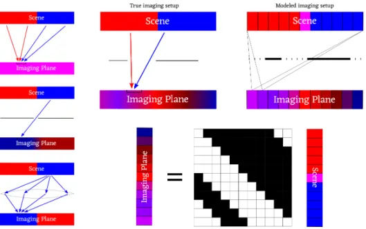
The second thing is that the standard way I index the scene vector is left-to-right, but the standard way I index the observation vector is right-to-left. (In a 3D world, I would reverse the labeling along both dimensions.) In principle, you could do everything I do in this thesis with the labeling of the observation going left-to-right, but it would make the analysis much less pleasant. See Figure 1-8 to see a side-by-side comparison of the true configuration and the modeled configuration.

1.4.1 The Transfer Matrix

Another critical concept in my dissertation is the transfer matrix. This is a standard concept in computational imaging, used when linearity can be established [103, 71, 72]. The transfer matrix is a matrix that describes the action of an aperture frame on the scene to create the observation. To be more precise, suppose we approximate the scene by a vector ⃗𝑥, where each entry of that vector gives the illumination of a single patch of the scene. Suppose that we approximate the observation plane in the same way with a vector ⃗𝑦. Then, the transfer matrix, 𝐴, will be whichever matrix satisfies