HAL Id: hal-03016661
https://hal.archives-ouvertes.fr/hal-03016661
Submitted on 20 Nov 2020
HAL is a multi-disciplinary open access archive for the deposit and dissemination of sci-entific research documents, whether they are pub-lished or not. The documents may come from teaching and research institutions in France or abroad, or from public or private research centers.
L’archive ouverte pluridisciplinaire HAL, est destinée au dépôt et à la diffusion de documents scientifiques de niveau recherche, publiés ou non, émanant des établissements d’enseignement et de recherche français ou étrangers, des laboratoires publics ou privés.
reflexive M&S studies
Bruno Bonté, Jean-Pierre Müller, Raphael Duboz
To cite this version:
Bruno Bonté, Jean-Pierre Müller, Raphael Duboz. Modeling the Minsky triad: A framework to perform reflexive M&S studies. 2012 Winter Simulation Conference - (WSC 2012), Dec 2012, Berlin, France. pp.1-12, �10.1109/wsc.2012.6465110�. �hal-03016661�
C. Laroque, J. Himmelspach, R. Pasupathy, O. Rose, and A. M. Uhrmacher, eds.
MODELING THE MINSKY TRIAD: A FRAMEWORK TO PERFORM REFLEXIVE M&S STUDIES
Bruno Bont´e
CIRAD-AGIRs and CIRAD-GREEN Presently at Lab. of Complex Systems Eng. (LISC)
IRSTEA - 24, av. des Landais BP 50085 63 172 Aubi`ere Cedex, FRANCE
Jean-Pierre M¨uller
Renewable resources and Env. Man. (GREEN) CIRAD - Campus de Baillarguet
34398 - Montpellier, FRANCE
Rapha¨el Duboz
Animals and Integrated Risk Management (CIRAD-AGIRs) Computer Science and I-Man. (AIT-CSIM)
AIT, 12120 Pathumthani, THAILAND
ABSTRACT
In this paper, we propose a general framework to evaluate models of systems that are ill defined, incompletely known, and furthermore, which cannot be experimented in real conditions, such as the economical systems at the country scale, epidemics (for obvious ethical reasons) or any natural disasters, for instance where human lives are the main issue. Our framework relies on the generic Marvin Minsky’s definition of a model and its specification in the frame of the Theory of Modeling and Simulation, initiated by B.P. Zeigler. Such a dynamic system vision of the Marvin Minsky model definition enables to address original questions using what we have called the Minsky triad model, i.e., a coupled model composed of the model of the user, the model of a real system, and the model of this later model. We think that the Minsky triad model is very promising as a framework to design decision support systems for crisis management.
1 INTRODUCTION
An important preliminary activity in modeling and simulation is to gather data from the source system we are interested in. Such data are used to build, to calibrate and to validate the model. Thereafter, we can learn from the model or forecast behaviors in order to be able to make decisions and to take actions on the system under study. A problem arises when the source system cannot be experimented for any reason. For instance, if we consider an epidemic in a human or animal population, we cannot experiment such a system for obvious moral and ethical reasons. Similar problems arise in many situations where human lives are the main issue. More generally and less dramatically, we can say that the systems defined at the ecological, economical or social scales (Socio-Eco-Systems, SES) cannot be experimented in most cases. A solution is to model a priori such systems, using a non validated model (or validated with previous similar situations) to support the decisions when a new situation occurs. In that case, we do not know if the model we are using would provide useful answers regarding to this new situation. In this paper, we propose a framework to address such an issue. The problem is to evaluate if a given model enables to make the appropriate decision in situations that have not been previously encountered. Furthermore, to be complete, such a framework should consider the interdependency between the source system dynamics and the actions the decision maker decides to perform on the source system based on this model. Indeed, in the context of SES systems, the objective of the decisions is to control the future trajectories of the system by acting on it, modifying in return the future trends of the system dynamics.
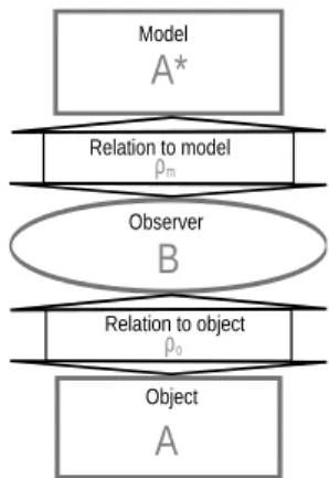
The framework we propose in this paper derives from the Marvin Minsky’s definition of what is a model. In 1965, M. Minsky said: ”To an observer B, an object A∗is a model of an object A to the extent that Bcan use A∗ to answer questions that interest him about A” (Minsky 1965). Starting from that definition, we call the “Minsky triad” T , the three entities A, B and A∗. Figure 1 represents this triad and the relations between the three entities that compose it. We call ρo and ρm the relations between the observer and the
object and between the observer and the model respectively. Such a representation is the first step towards a systemic conception of the triad.
Object
A
ObserverB
ModelA*
Relation to model ρm Relation to object ρoFigure 1: The Minsky triad T .
The next section will present the general conceptual framework (Section 2). Then we will present more specifically the model of the triad using the Theory of Modeling and Simulation (Section 3). We will illustrate the use of this framework on a specific case in Section 4. We will then discuss the results and conclude in Section 5.
2 THE GENERAL FRAMEWORK
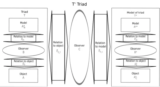
The Figure 1 illustrates the classical relation among a model, the source system and the user of the model, as a Minsky triad T . The main idea of this work is to model the Minsky triad itself, leading to a reflexive representation to address questions related to the use of models. Therefore, in order to study the interactions among the three entities of the triad, we propose to build a model T∗of the triad T . Doing that, we create a new triad in which the source system is the triad T , the observer is the researcher C and the model is the model T∗. This last triad is the general conceptual framework that we propose for model evaluation. We note T0 this framework and present it in Figure 2 page 3. In order to address questions about the use of model A∗B, the observer C builds a model T∗ of the triad T . ρo c is the question C has on T . ρm c is
the experimentation (i.e. the simulations) C performs on T∗. In this framework, the question of C will not be about the model A∗B, but about the use of the model A∗B by B, as far as the model AC∗ represents the behavior of A. Consequently, the T∗ model must contain a model of each entity and relation present in the triad T : AC∗ is a model of entity A for observer C and A∗B is a model of entity A for observer B, A∗∗ is
both a model of AC∗ for B∗ and a model of A∗B for the observer C. Finally, ρo∗ is the model of the relation
ρo and ρm∗ is the model of the relation ρm.
Having this general framework, we can use the concepts and formalisms from the Theory of Modeling and Simulation (TMS) initiated by B.P. Zeigler (Zeigler, Kim, and Praehofer 2000) to specify the model of the Minsky triad T∗, and to design and implement the corresponding simulator. Indeed, we could directly build a morphism between the entities of the Minsky triad including their relations on the one hand, and the models specified using the Discrete EVent systems Specification (DEVS) formalism on the other hand. In our framework, the model of the observer B∗ has to manipulate the model A∗∗ in order to make decisions on the model of the source system A∗C. The main difficulty here is in the formalization of
T' Triad Observer C Relation to model ρm_c Relation to object ρo_c Object A Observer B Triad T Model A*B ρ Relation to model m Relation to object ρo Model of triad T* Observer B* Model A** Object A*C Relation to model ρm* Relation to object ρo*
Figure 2: The general framework T0.
the use of a model by another model. Indeed, when an observer uses a model to make decisions, the model has its own simulation time line, which is different from the time line of the model user. To tackle this particular problem, we have proposed the use of the recursive simulation technique described in a previous study (Bont´e et al. 2009). This technique is combined to the concept of experimental frames in order to specify the experiments that B∗ performs on A∗∗. In the TMS, any question about a dynamic system should be related to an experimental frame (Zeigler, Kim, and Praehofer 2000; Traore and Muzy 2006). The experimental frame specifies the system environment, or “context of interest”. It basically specifies the input signals sent to the system (or to the simulator) and the observation policy, i.e. the simulation outputs that are monitored. For example, any validation process consists in comparing the behavior of the system with the behavior of the model within the experimental frame related to the question we have on the system.
In the following, we present a possible specification of the T∗model using the TMS and more specifically the DEVS formalism.
3 THE T* DEVS MODEL
The DEVS formalism enables to specify the T∗ model as a generic hierarchical structure. Within this structure, some models of sub-processes are generic and others can be specified and reused at will, thanks to the modularity feature of the DEVS formalism.
The A∗C model is a DEVS model. The ρo relation between the observer and the source system is
formalized as a set of Sub-Processes for Observation and Control (SPOC). Its model is ρo∗. For instance,
it can be composed of a model of observation and a model of action coupled together.
Considering A∗B is a model of a dynamic system, we can design a simulator to simulate it. We consider that a simulation is a virtual experiment. Doing so, the ρm relation between the observer and the model
is considered as an experimental process performed on the A∗B model by B. The corresponding ρm∗ model
in Figure 2 page 3 is consequently called the Experimentation Process Model (EPM). It models the ρm
relation between the observer and the model. The EPM is an important piece of our framework. B.P. Zeigler gives the following definition of a dynamic system simulation model: ”A simulation model [...] is a set of instructions, rules, equations or constraints allowing to generate an Input/Output (IO) behavior”. In our case, one can imagine the A∗B model as a set of rules or equations. The dynamic system model describes a dynamic system behavior, but it is not a dynamic system itself. By opposition, a dynamic system actually generates IO behavior. Therefore the dynamic system described by A∗B cannot directly
interact with any triad sub-systems. These equations or rules cannot be coupled with the other sub-systems of the triad. A∗B can only be simulated. Likewise, the EPM cannot directly interact with the A∗∗ model by sending events to it because A∗∗ stays a model (a set of instructions, rules etc., and not a physical dynamic system) within the T∗ model. To perform experiments that require dynamic interactions with the dynamic system described by A∗∗, the EPM needs to build an Experimental Frame (EF), which is a model of dynamic system itself, and which is simulated in the same simulation time line as the A∗∗ model. We explain in (Bont´e et al. 2009) how such EPM can be built by using the recursive simulation technique. Another specification which takes better benefice of the EF concept is described in (Bont´e 2011). The EPM enables to specify this special interaction between the dynamic system described by the A∗∗ model and those described by the models of the triad sub-systems.
Finally, the B∗model is reduced to the decision process that the observer B performs to influence the SPOC, according to information obtained from the experiments realized with the A∗B model.
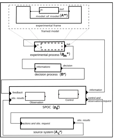
A proposal for a general structure of T∗ using DEVS is presented in Figure 3. The rectangular boxes represent dynamic system models, specified either as atomic DEVS models or composed DEVS models. The lines between boxes represent connections between models that can be either “port → port” connections or “model → model” connections (meaning one or several “port → port” connections). We did not represent any connection within the ρo∗ model because the Observation and Action sub-models are just given as an
example of SPOC components. The decision process model receives information from the ρm∗ model and
can influence the ρo∗ model behavior. The ρm∗ model is an experimentation process model. It embeds the
A∗∗ model and experiments it using an experimental frame.
4 EXAMPLE OF APPLICATION OF THE FRAMEWORK
4.1 Introduction: Evaluation of Model Use in Animal Epidemiology
In order to discuss the interest of our framework, we explain how it can be used in the context of animal epidemiology. Diseases spread in a human or an animal population is a good example of a non experimentable system. Furthermore, modeling and simulation is widely used in epidemiology.
Many of the processes involved in diseases spread are identified and are similar from an epidemics to another. However, the qualitative knowledge of theses processes is not sufficient to predict the system evolution. An accurate knowledge of the relative weights of each process is necessary. The problem is that this knowledge will be available only after the epidemics has occurred. Moreover, people may neither just let some disease spread with no reaction. Consequently the observer is part of the system and cannot stay passive. The surveillance system must be considered in any disease spread analysis (H¨ohle, Paul, and Held 2009) because the epidemics itself cannot be directly monitored. The issue is that the epidemics dynamics may depend on the surveillance system designed to observe it.
With the increasing use in M&S in epidemiology, we have many information on triads used in this field and some systematic reviews have been published (Singer 2010; Singer, Salman, and Thulke 2011). Considering the source system A, most of the processes involved in disease transmission and spread have been precisely described, leading to precise characterization of epidemics systems considered at different scales. Considering the A∗Bmodel huge work has been done to simulate disease spread and several classes of models exist (Keeling and Rohani 2007). Considering the observer B, it is composed of the network of decisional institutions (such as OIE, national veterinary or human health departments) and research teams. We can observe how the decision process tells which management policy must be applied according to information gathered from the use of model A∗B. The ρo relation between the observer and the source
system is precisely described as a combination of a surveillance system and a control system. Considering the ρmrelation between the observer and the model, many kind of experimental plans have been designed
and are described in the literature in order to perform calibration, optimization or sensitivity analysis for instance.
decision experimental process in out feedback information Control decision process informations framed model out in model of model experimental frame SPOC source system(A *)C (ρ *)o (B*) m (ρ *) (A**) Observation control and observations request obs. results obs. results actions and obs. request
Figure 3: The T* DEVS structure.
As explained previously, the models themselves can hardly be evaluated in regards to their capacity to reproduce the source system behavior. Nevertheless, we can evaluate the use of specific models in specific situations. Thanks to all information concerning model use in epidemiology, we are able to build reliable simulation models of these situations. In this section, we present how the formal model presented in Section 3 can be used to evaluate the model use in the case of animal epidemiology. We use the conceptual framework presented in Section 2 to organize our discourse. Alike the general case of triad of triad presented in Figure 2 page 3 we consider three triads. The first triad T is a usual situation where the A entity is an epidemic, the B entity is a surveillance and control system and the A∗entity is an epidemiological model. The second triad T∗ is a model of the T system. Finally, the third triad T0 is composed of the T system, the T∗ model and the research questions we have on T .
4.2 T : Surveillance, Modeling and Control of an Epidemics
In this application we consider a triad T where an epidemics is observed by a surveillance system and control by a control system. An epidemiological model is used to set the level of control. Recall that the T system is composed of a system A, a SPOC (ρo), a decision unit B and a model experimentation
process (ρm) using a model A∗. We will refer to the A system as the epidemiological system. It is a
set of a hundred epidemiological units (sub-regions of a geographical area of interest) connected to each other by an infectious contact network through which an infectious epidemiological unit can infect its
acquaintances. The SPOC is a system for epidemiological surveillance and control and is composed of a passive observation system, a proactive observation system and a control system. The passive observation system observes all components of the epidemiological system until an outbreak is detected. When an outbreak is detected, the proactive observation system and control system are activated. The control consists in reducing the movement of animals in the area of interest. Several levels of movement restriction are defined corresponding to different intensity of control. At first a default level is chosen, then the control system can modify the level of movement restriction following the decision system. Note that the level of control is known (it can be quantified as the number of animals allowed to be moved from one place to another for instance) but the impact it has on the disease spread is unknown. The proactive observation system observes at regular time step a representative sample of epidemiological units in order to estimate at each time step the prevalence in the area of interest. (The prevalence in a population is the proportion of infected individuals in this population). This information is then sent to the model experimentation process. The model experimentation process uses a SIS model (Anderson and May 1979) consisting in calibrating the model by using available data (prevalence estimation from the observation system). An interesting feature of the SIS model is that its dynamics is characterized by the R0 indicator (Keeling and
Rohani 2007). When R0> 1, a stable state is reached corresponding to a non null proportion of infectious
individuals in the population equal to 1 − 1/R0. On the other hand, if R0< 1 the proportion of infectious
individuals will tend to zero. The decision system receives the calibrated model from the experimentation process and computes the corresponding value of R0 from this model. The decision system increases or
decreases the control level according to the value of R0.
4.3 C: a Set of Questions Related to Model Use in Epidemiology
There are several questions for which we can hardly find answers within T but which we can ask as an external observer. Within the T0 triad, we choose three questions to represent different types of questions that we have on T as an external observer (observer C in Figure 2) and to which we will try to answer using the model T∗. The issues we want to address about T as the observer C of the T0 triad are the following: 1. What is the impact of the epidemiological surveillance system on the production losses due to the
disease?
2. What is the impact of the model experimentation process on the production losses due to the disease? 3. How these impacts depend on the epidemiological system of interest?
Type 1 questions deal with the design of the passive and proactive observation systems (ρorelation). Type 2
questions deal with the design of the model experimentation process (ρmrelation). Finally, type 3 questions
deal with the compatibility of the surveillance, control and model experimentation processes (ρo and ρm)
with the nature of the epidemiological system of interest (A). All the questions deal with the consequences that the design of the surveillance, control and modeling of the disease may have on the disease (possibly considering the nature of the disease for type 3 questions).
In the T system, we identify factors that we can use to characterize different design modalities of the surveillance, control and model experimentation processes on the one hand, and different scenarios of diseases on the other hand. We also identify criteria to evaluate the consequences of the disease in terms of production losses and to evaluate quantitatively the surveillance and control effort. We choose the transmission rate between epidemiological units as a factor that would characterize the epidemiological system. It can be measured using the mean spreading speed between two neighbor units. We choose the sampling time period of the proactive observation system as a factor that would characterize the design of the surveillance system, It is measured as the time step between two successive sampling. As a factor that would characterize the model experimentation process we choose the binary answer to the question: ”do we know the value of the γ parameter of the SIS model for this disease?” (see equations 1 and 2). We choose two criteria to characterize the production loss due to the disease. The first is the cumulative time of
infected epidemiological units measured as the total number of infected epidemiological units multiplied by the time they have been infected. The second is the quarantine length of the whole geographical area measured as the time period between the first detected outbreak and the last detected outbreak. Finally, as a criteria that would characterize surveillance and control cost, we choose to measure the surveillance effort as the total number of epidemiological units sampled by the proactive surveillance system and the control effort as the integral of the control intensity.
4.4 T∗: the Simulation Model of T
The interest in building the T∗ simulation model is two sided. First, some of the factors or criteria are not directly measurable in T . It is the case for the cumulative time of infected epidemiological units for instance. Second, the T∗ model enables us to realize proper experimental plans allowing to empirically evaluate the influence of the factors values over the criteria values. The structure of the T∗model is similar to the generic one presented in Figure 3 page 5. Due to lack of space and because our objective is less to present quantitative results than a methodology, we do not present all details of the T∗ model. Note that these details are given, as well as a complete DEVS specification, in the PhD dissertation of the first author (Bont´e 2011). However we must note some important points in order to discuss the simulation results.
Concerning the model of the epidemiological system, note that each epidemiological unit is modeled as a DEVS model and that the infectious contact network is the connection graph between IN/OUT ports of these models. Each model of an epidemiological unit is a two states automaton whose states are either Susceptible (S) or Infectious (I). In state I, an epidemiological unit can infect its neighbors in state S with an infection rate noted rin f. The passive observation process model is connected to all epidemiological
units model and detects a switch to an I state with a given detection probability. The proactive observation process model connects itself at regular time step to a sample of epidemiological unit models. The number of sampled epidemiological units is computed at each observation time step according to the prevalence observed at the previous observation time step, a desired relative precision and a statistical formula ordinarily used to compute the sample size in epidemiological surveys. The model of control modifies the infection rate rin f of all epidemiological units by multiplying it by a factor chosen in a collection of numbers
corresponding to different control levels. The A∗∗model is the SIS model given by the equations 1, and 2. The experimental frame used consists in setting the initial state and parameters and to observe the dynamics of the I state variable.
dS
dt = γ I − β IS (1)
dI
dt = β IS − γ I (2)
where
{S, I} ∈ R2 are the two state variables (representing respectively the proportion of susceptible and
infectious individuals in the population),
β and γ are two parameters (respectively the infection rate and the recovery rate).
The EPM implements a swarm particle optimization algorithm which enables to estimate the values of β (and possibly the value of γ if the recovery rate is unknown) that enable the best fit between SIS simulation results and the time series observed by the proactive observation model. The decision model B∗, uses β and γ values to compute the R0 indicator (R0= β /γ). If R0> 1, the control intensity is increased
to the superior level. If R0 tol< R0≤ 1, the control is unchanged. If R0≤ R0 tol, the control intensity is
decreased to the inferior level. We consider that the level of control is known by the decision maker but the corresponding factor applied to the infection rate rin f is unknown.
4.5 ρm c: Simulation of T∗
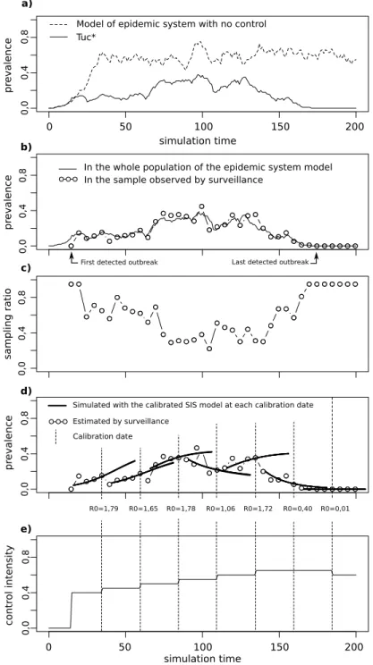
The T∗model is stochastic so we can get several different simulation results using the same set of parameters and changing the random number generator seed of the simulator. In this section we comment the results of a single simulation. Figure 3 page 5 presents the simulation outputs for this simulation.
Model of epidemic system with no control
R0=1,79 R0=1,65 R0=1,78 R0=1,06 R0=1,72 R0=0,40 R0=0,01 Estimated by surveillance
Simulated with the calibrated SIS model at each calibration date
Calibration date
In the sample observed by surveillance a)
b)
c)
d)
e)
First detected outbreak
pr eva len ce simulation time pr eva len ce
In the whole population of the epidemic system model
sa mpli n g rat io pr eva len ce simulation time co n tr ol i n ten sity
Last detected outbreak
Tuc* 0 50 100 150 200 0 50 100 150 200 0, 0 0 ,4 0, 8 0, 0 0 ,4 0, 8 0, 0 0 ,4 0, 8 0, 0 0 ,4 0, 8 0, 0 0 ,4 0, 8
4.5.1 Trajectory of the Epidemiological System
On the a) chart, we see the evolution of prevalence in the model of epidemiological system (plain curve). The dashed curve shows an example of prevalence evolution for the simulation of the model of epidemiological system with no control. We observe that the epidemics ends when the system is controlled (prevalence is null at the end of the simulation for the plain curve), although in the case with no control, the disease becomes endemic (prevalence seams to become stable around a positive value for the dashed curve). 4.5.2 Trajectory Perceived by the Surveillance System
Chart b) shows prevalence values estimated by the proactive observation model (dots). It corresponds to the prevalence observed in the samples. The “real” prevalence in the model of epidemiological system is plotted as a plain curve. We observe that both curves are very close. Distance in time between the estimated prevalence dots corresponds to the sampling time period of the proactive observation model. The date of the first prevalence estimation corresponds to the activation of the proactive observation model triggered by the first outbreak detection by the passive observation model. We notice that this activation occurs a short time after the epidemic starts (the plain curve is already increasing).
4.5.3 Trajectory of an Indicator of the Proactive Observation Model Activity
Chart c) shows the proportion of epidemiological units sampled at each sampling performed by the proactive observation model (recall that the number of units to sample is computed by the proactive observation model at each observation time step). We notice that variations are wide.
4.5.4 Information Brought by the EPM
Chart d) shows the results obtained by the EPM. The prevalence data estimated by the proactive observation model have been replotted (dots). Recall that calibrations performed by the experimentation process model are based on these data. The vertical dashed lines mark the dates at which calibrations occurs (the EPM perform a calibration each time 5 new prevalence data are available). For each calibration, the prevalence evolution simulated with the calibrated SIS model has been plotted (plain short curves) from the date of the first observation used for this calibration (five observations before), until a prediction horizon fixed to the time between two calibrations. The R0 value computed for each calibration is written below each
calibration date. Note that the prevalence simulated with the SIS model fits very well the surveillance data (the five prevalence observations preceding a calibration are almost superimposed with the corresponding SIS simulation curve), and predicts badly the future prevalence (observations following a calibration can be very far from the SIS simulation curve corresponding to this calibration). This last result is expected because the control level following a calibration may be different of the control level preceding the calibration. 4.5.5 Trajectory of an Indicator of the Control Model Activity
Chart e) shows the evolution of the control intensity during the simulation. Note that the control model is activated at the same time as the proactive observation model (the control intensity is 0 before the first prevalence value is observed on charts b), c) and d). At each calibration, the control level is revised. It is increased if the estimated R0is superior to 1 (which is true until the penultimate calibration), maintained
if Ro tol< R0< 1 (which is true at the penultimate calibration), and decreased if R0≤ R0 tol which is true
for the last calibration. 4.5.6 Experimental Plan
In a M&S approach, we transfer the questions we have on T to T∗ and we perform an experimental plan on T∗. We performed a light experimental plan on T∗ in order to show that we can formulate questions
of type 1, 2 and 3 presented in Section 4.3 as experiments on T∗. This is an empirical approach leading to statistically measure the influence of our factors on our criteria.
Notice that we can compute our criteria from simulation outputs. For instance, the quarantine duration criterion can be measured on the chart a) of Figure 4 as the duration between the first detected outbreak and the last detected outbreak. The surveillance effort criterion can be measured on chart c) as the sum of all sample sizes. For a given set of parameters and a few modalities tested on our factors, we performed thirty simulations for each factors combination. As an answer to “type 2” and “type 3” questions, we could show that for the tested modalities, knowing the value of the γ parameter (fixing γ and calibrating only β instead of calibrating both β and γ parameters with the EPM) has no significant impact on the cumulative infected time in the scenario of a slow disease spread but had a significant impact in the case of a fast disease spread.
For the same set of parameters we also found that decreasing the proactive sampling time period significantly decreased our surveillance effort indicator for the same value of our control effort indicator. This result is counter intuitive because more epidemiological units are sampled by time units if sampling time period is lower. This is due to the fact that epidemics are in average shorter if the sampling is more frequent (control is more efficient). This kind of answers to questions of type 1 give a different (and we think interesting) point of view on monitoring systems which are usually evaluated on their capacity to capture the epidemic trend and not as a part of the epidemics dynamics.
4.6 ρo c: Potential Answers on T
4.6.1 Validation of T∗
Our motivation to build the model T∗ is that the model A∗B cannot be validated. However, note that the system T contains the source system A. Consequently, we could think we would not be able to build a validated AC∗ model. At that point, it is important to notice that the questions we want to address with the AB* model are not the same that those we want to address with the AC∗ model. In the T triad, the A∗B
model is used to produce a summary of the A system (the R0 indicator in our case). In the T0 triad, the
AC∗ model is used to reproduce the complexity of the A system in order to evaluate if the SIS model is able to produce a satisfactory summary of the disease dynamics. The summary is considered satisfactory depending on the efficiency of the control that it enables to perform. In the case of the T∗ model we presented, we consider that the A∗Cis valid to represent the complexity due to non-homogeneous mixing of the population. Indeed, epidemiological units are connected via a network of infectious contact that may not be random (we choose a 2D regular lattice network for the shown simulations). Consequently, T∗ is valid if we use the AC∗ model as a sufficient informative hypothesis. Then, under the hypothesis of AC∗, the answers we have by experimenting T∗ can be transferred to T . For this reason, we think that the most interesting questions to address with the T∗ model are those of type 3, i.e. evaluating different types of models integrated in different situation of disease management.
4.6.2 Learning on T and Offered Perspectives
The example of application given in this paper only showed that, under the AC∗ hypothesis, model evaluation can be based on the efficiency of the control the model enables. Intensive experimental plans must now be performed to bring reliable results to the epidemiological modeling community. The first type of results would be recommendations about which kind of model (spatial or not, aggregated or individual based) and model experimentation process could be used depending on the epidemics situation (fast or low infection rate of the disease, availability of surveillance effort, ... ). The second type of results is to help designing new T systems that cannot have been designed already because they cannot have been tested yet. We think that experimenting on T∗ can help to design new surveillance and control systems based on simulation model results. Finally, T∗ can support epidemiologists training by reproducing some of the mechanisms leading to wrong model predictions.
5 DISCUSSION AND CONCLUSION
In this paper, we proposed a conceptual, formal and operational framework to evaluate models of systems that cannot be experimented. This is an important issue in the field of modeling and simulation of large scale complex systems in disciplines such as economy, ecology, sociology etc. We are facing huge challenges for the future, and we have to make important decisions. Unfortunately, we can not use the classical experimental approach for such systems. Indeed, a classical validation process based on comparing system and model behaviors within an experimental frame is here meaningless. Consequently, it is hardly possible to evaluate decisions based on model uses.
To deal with this issue, we have proposed a new methodology to evaluate the use of simulation models. We proposed to model the whole Minsky triad composed of three entities: the object (or source system), the observer and the model. Doing so, we represented the feedback loop between decision made using a model of a source system, and the source system itself. Therefore, such a framework can be used to model, and then to test, a priori decision making process in a context where experimentation is not possible. The first contribution of this work is then a methodology based on the conceptual framework presented in Section 2, illustrated Figure 2 and instantiated Section 4. The fundamentals of this methodology are to use the TMS to enable a reflexive study of the TMS activity, in order to improve its uses in problematic cases. The second contribution is the generic T∗ model presented in Section 3. Even if this paper only draws the main lines of a generic T∗ model, it offers a strong basis which can be improved in the frame of the TMS, notably considering all the works already done in concern with the experimental frame specification. The EPM presented in (Bont´e 2011) is generic. Nevertheless, it needs to face more applications. Note that using DEVS formalism to specify T∗ allows to build triads using existing models. It is a particularly interesting feature for AC∗ and A∗∗. Finally a third contribution is the demonstration that recursive simulation can be achieved within a DEVS simulator. All the computer developments have been done using the Virtual Laboratory Environment (VLE) (Quesnel, Duboz, and Ramat 2009) which provides all the necessary features to design, implement and analyze DEVS models. VLE is based on the concept of packages to enable the model developers to share their development. For this work, a package called “experimenter” has been developed for the EPM.
The reader has probably noted the risk of circularity in our approach, because the source system seems to disappear in the proposed framework. In fact it is not the case. In practice, we have a collection of models of the source system that have been built and validated in similar situations; we have hypothesis on the processes and empirical knowledge on the source system. It is therefor possible to simulate a wide variety of source system behaviors, and to select the simpler and most accurate model we can use to make a decision in a particular context. To do that, we propose to introduce the experimental approach in the framework to perform a type of sensitivity analysis not only with the model parameters, but also with the model structure. The experimental approach is at the basis of science. Using this approach should gradually increases the understanding we have on the source system. This may be the only way to address some essential questions about the use of models for decision making in crisis management. We emphasized this issue with the example of model used for epidemics management and we are convinced that this work shall give rise to a new kind of model evaluation in contexts where experiment is not possible, such as financial crisis management, epidemiology, or climate change for instance. We hope that new kinds of model based decision support will arise thanks to a better evaluation of these models and models uses. ACKNOWLEDGMENTS
The authors sincerely thank the three reviewers of this paper for their careful reading, wise advices and patience. They also thank Fr´ed´erick Garcia and Mamadou Kaba Traor´e for their advices about the use of a Minsky triad model.
REFERENCES
Anderson, R. M., and R. M. May. 1979. “Population biology of infectious diseases: Part I and II”. Nature280:361–367.
Bont´e, B. 2011, December. Modelling and simulation of interdependence between the object, the observer and the model of the object in the triad of Minsky. Application to animal health surveillance.Ph. D. thesis, Universit´e Montpellier II. PhD in french with summary in english.
Bont´e, B., R. Duboz, G. Quesnel, and J.-P. Muller. 2009. “Recursive simulation and experimental frame for multiscale simulation”. In Proceedings of the Summer Computer Simulation Conference, SCSC ’09, 164–172. Vista, CA: Society for Modeling & Simulation International.
H¨ohle, M., M. Paul, and L. Held. 2009. “Statistical approaches to the monitoring and surveillance of infectious diseases for veterinary public health”. Preventive Veterinary Medicine 91 (1): 2–10. Keeling, M., and P. Rohani. 2007. Modelling Infectious Diseases In Humans And Animals. Princeton
University Press.
Minsky, M. 1965. “Matter, Mind and Models”. In Proceedings of IFIP Congress, edited by I. F. of Information Processing Congress, 45–49.
Quesnel, G., R. Duboz, and ´E. Ramat. 2009. “The Virtual Laboratory Environment – An operational framework for multi-modelling, simulation and analysis of complex dynamical systems”. Simulation Modelling Practice and Theory17:641–653.
Singer, A. 2010. “External report reviewing the previous opinions of the Panel on Animal Health and Welfare concerning the application of quantitative tools, in thesequence of the current self mandate on Good Practice in ConductingScientific Assessments in Animal Health Using Modelling”. Technical Report No EFSA-Q-2009-408, European Food Safety Authority, Parme, Italie.
Singer, A., M. Salman, and H. Thulke. 2011. “Reviewing model application to support animal health decision making”. Preventive Veterinary Medicine 99 (1): 60–67.
Traore, M. K., and A. Muzy. 2006. “Capturing the dual relationship between simulation models and their context”. Simulation Modelling Practice and Theory 14:126–142.
Zeigler, B. P., T. G. Kim, and H. Praehofer. 2000. Theory of modeling and simulation: Integrating Discrete Event and Continuous Complex Dynamic Systems. Academic Press.
AUTHOR BIOGRAPHIES
BRUNO BONT ´E is a post-doctoral student scholar in the French Institute of Science and Technology for Environment and Agriculture. He recently received his doctorate in Computer Science from the University of Montpellier II. His PhD was realized in the French Center for International Cooperation in Agricultural Research for Development (CIRAD) and co-supervised by J.P. M¨uller and R. Duboz. His research inter-est are M&S applied to Socio-Ecological-System management and understanding. [email protected]. JEAN-PIERRE M ¨ULLER is senior scientist at CIRAD (France) since 2001, focusing on multi-agent modeling of socio-ecosystems applied to renewable resources management. His current research is partly embodied into the MIMOSA platform. Computer science Professor at the University of Neuchˆatel (Switzer-land) from 1987 until 2001, he co-founded the European community on multi-agent systems (MAAMAW workshops). He is author of more than a hundred publications in the field. [email protected]. RAPHA ¨EL DUBOZ is a Visiting Assistant Professor at the Asian Institute of Technology (AIT) in Bangkok, Thailand. He has been seconded by CIRAD, where he served as a researcher in modeling and simulation with applications in animal epidemiology. He has more than 10 years of experience in computer modeling and simulation. His current main interests are in discrete event systems, complex systems modeling, including qualitative modeling, companion modeling and networks analysis. [email protected].