HAL Id: hal-00736576
https://hal.archives-ouvertes.fr/hal-00736576
Submitted on 28 Sep 2012
HAL is a multi-disciplinary open access archive for the deposit and dissemination of sci-entific research documents, whether they are pub-lished or not. The documents may come from teaching and research institutions in France or abroad, or from public or private research centers.
L’archive ouverte pluridisciplinaire HAL, est destinée au dépôt et à la diffusion de documents scientifiques de niveau recherche, publiés ou non, émanant des établissements d’enseignement et de recherche français ou étrangers, des laboratoires publics ou privés.
H. Abdallah, N. Baghdadi, Jean-Stéphane Bailly, Y. Pastol, F. Fabre
To cite this version:
H. Abdallah, N. Baghdadi, Jean-Stéphane Bailly, Y. Pastol, F. Fabre. Wa-LiD: A new LiDAR sim-ulator for waters. IEEE Geoscience and Remote Sensing Letters, IEEE - Institute of Electrical and Electronics Engineers, 2012, 9 (4), p. 744 - p. 748. �10.1109/LGRS.2011.2180506�. �hal-00736576�
Wa-LiD: A new LiDAR simulator for waters
Hani Abdallah1, Nicolas Baghdadi1, Jean-Stéphane Bailly2, Yves Pastol3, Frédéric Fabre4
1
CEMAGREF, UMR TETIS, 500 rue François Breton, 34093 Montpellier Cedex 5, France.
2
AgroParisTech, UMR TETIS, 500 rue François Breton, 34093 Montpellier Cedex 5, France.
3
SHOM, CS 92803, 29228 Brest Cedex 2, France
4
EADS – Astrium, 31 rue des cosmonautes, 31402 Toulouse Cedex 4, France Email : [email protected]
Phone: +33 467548719, Fax: +33 467548700
A simulator (Wa-LiD) was developed to simulate the reflection of LiDAR waveforms from water across visible wavelengths. The specific features of the simulator include (i) a geometrical representation of the water surface properties, (ii) the use of laws of radiative transfer in water adjusted for wavelength and the water’s physical properties, and (iii) modelling of detection noise and signal level due to solar radiation. A set of simulated waveforms was compared with observed LiDAR waveforms acquired by the HawkEye airborne and GLAS satellite systems in the near-infra red or green wavelengths and across inland or coastal waters. Signal-to-noise ratio (SNR) distributions for the water surface and bottom waveform peaks are compared with simulated and observed waveforms. For both systems (GLAS and HawkEye), Wa-LiD simulated SNR conform to the observed SNR distributions.
Index Terms— Waveform model, altimetry, bathymetry, SNR, GLAS, ICESat, HawkEye
I. INTRODUCTION
Water surface altimetry and bathymetry are key variables for many applications in hydrology, geomorphology and meteorology (e.g., [1], [2]). Several techniques for measuring water altimetry and bathymetry have been developed through the use of sonar, radar and optical imaging. Each of these techniques has drawbacks when used on inland or coastal waters [3], including (i) limited spatial coverage and use on navigable rivers (sonar), (ii) a large radar footprint when used for inland water, especially rivers and (iii) the lack of the use of optical imaging in unclear waters.
Airborne hydrographic LiDAR has proved to be a suitable sensor because of its accuracy and high spatial density features [4]. The potential for airborne hydrographic LiDAR is that it can be used for both altimetry and bathymetry because of the ability of LiDAR detectors to register returned signals from (i) the water surface for altimetry [5], (ii) the water bottom for bathymetry ([6], [7]), and (iii) the water column that allows some optical properties of water to be deduced [8]. The Airborne Hydrographic LiDAR technique is limited in terms of spatial coverage and because the data is expensive to gather.
ICESat has been the only altimeter LiDAR satellite up to now. The Geoscience Laser Altimeter System (GLAS) from ICESat provides accurate high resolution elevations for altimetry. The GLAS is promising for inland areas with widths greater than 1.5 km, even though the footprint is small (50 to 90 m), because of the time needed for detector gain adaptation when transitioning from land to water (0.25 s, approximately 1.5 km). The transition phase from land to water limits the use of GLAS in small, inland water areas [9].
To improve the prospective and the performance analysis in satellite LiDAR systems designed for water altimetry and bathymetry, a LiDAR signal database representative of the possible physical conditions of water using different LiDAR configurations is needed. The common procedure to obtain a
database involves the development of a physical model simulating the signals. Such a model would allow the reproduction of the LiDAR signal regardless of the water and instrumental parameters.
Most hydrographic applications that use LiDAR signals are derived from the work of Guenther [5]. Before now, few studies have been published that model LiDAR waveforms on water; these studies include (i) the simulation model of Mclean [10], which generates LiDAR returned waveforms from a wind-roughened ocean, (ii) the work of Feigels [6] on the optimisation of airborne LiDAR’s parameters through modelling and analysing waveforms and (iii) work on modelling sea surface return and laser bathymetry from airborne LiDAR [7].
The objective of this study is to develop a new waveform simulation model available for any laser wavelength in the optical spectrum domain from 300 (Ultra Violet, UV) to 1500 nm (Near Infra Red, NIR). This model is similar to other Hydrographic LiDAR models (e.g., [5], [6], [7]) except it integrates radiative transfer laws governed by the physical properties of water for any wavelength. This simulation model uses a geometrical representation of the water surface with the geometric model of Cook and Torrance [11] and integrates both the characteristics of detection noise and signal level due to solar radiation.
The aim of this paper is (i) to present the water LiDAR waveform model (Wa-LiD) formulae regardless of LiDAR system parameters and water parameters, (ii) to exhibit a selection of simulated waveforms for certain wavelengths and the same water characteristics and (iii) to compare simulated waveforms to observed LiDAR waveforms from the satellite GLAS sensor and the airborne HawkEye sensor.
II. LIDAR MODELLING
A. The Water LiDAR (Wa-LiD) Simulation Model
1) Model description
The Wa-LiD model is able to simulate waveforms for any laser wavelength in the optical spectrum domain from 300 to 1500 nm regardless of the optical properties of water. These optical properties are determined by the attenuation (absorption + scattering) of optical light by pure water, yellow substances, phytoplankton and sediment (e.g., [12], [13]). In addition, this Wa-LiD model (i) takes into account any Bragg-scattering from the water surface using the geometric (facets) model of Cook and Torrance [11] and (ii) integrates the effects of detector noise and noise due to solar radiation.
The waveforms received by the LiDAR system (power as a function of time) are written as the sum of the echoes of multiple waves [7]:
PT(t) = Ps(t)+ Pc(t)+ Pb(t) + Pbg(t)+ PN(t) (1)
Where PT(t) is the total power received, Ps(t) is the power
returned by the water surface, Pc(t) is the power returned by
the water column, Pb(t) is the power returned by the bottom,
Pbg(t) is the background power returned by the air column,
PN(t) is the detector noise power and t is the time scale.
The emitted laser pulse from the LiDAR system is considered to be a Gaussian distribution [14]:
(
Τ ²)
)² t -(t 0 x 0 x 4ln2 -exp π 2 ln T 2 ) t ( w = (2)Where tx is the two-way time delay of the emitted Gaussian
pulse between the detector and the water surface ts, water
column tc or bottom tb. The returned waveforms from the water
surface, water column and bottom correspond to the convolution of the Gaussian emitted pulse and the instant echoes from the water surface Ps, water column Pc and bottom
Pb.
Returned waveform from water surface:
The returned waveform from the water surface received by the LiDAR detector Ps(t) is given by: Ps(t) = w(ts) * Ps, with:
2 2 S R e R 2 atm e S H π ) θ ( cos L η η A T P P = (3)
Pe is the emitted power by laser = E0/T0, E0 is the emitted
energy of the LiDAR system, T0 is the Gaussian FWHM (Full
Width at Half Maximum), Tatm2 is the two way atmospheric loss, AR is the receiver area, ηe and ηR are the optical
efficiencies of emission and reception, LS is the loss of
transmission through the surface (surface albedo), θ is the local incidence angle, H is the sensor altitude,
) θ cos( c H 2 ts= ,
and c is the velocity of light in air.
The loss factor through the surface LS is calculated by the
BRDF (Bidirectional Reflectance Distribution Function) of the water surface represented by specular microfacets using the geometric model of Cook and Torrance:
θ cos π DOF k π k LS = d + s 2 r (4)
kd and ks (kd = 1 - ks) determine the fraction of diffuse and
specular components, respectively. D is the microfacet distribution function that models the surface as geometric facets and is described by the distribution function of Beckmann [15]. (tanθ/r)2 4θe cos ² r 1 D = (5)
r is the rms (root mean square) slope of the facets, which
determines the surface roughness. Small values of r signify gentle facet slopes and give a distribution that is highly directional around the specular component while large values of r imply steep facet slopes and give a distribution that is spread out [11].
O is the geometric attenuation factor of the BRDF that takes
into account the phenomenon of masking between facets (auto-shadowing). Fr is thefunction that describes the Fresnel
reflection of light on each microfacet.
Returned waveform from water column
The returned waveform from the water column PC(t) at a
depth z is given by: Pc(t) = w(tc) * Pc(z), with:
(
)
(
)
2 θ cos z H n θ cos kz 2 2 s R e R 2 atm e c w w exp ) φ ( β ) L 1 ( F η η A T P ) z ( P + -= (6)θw is the local incidence angle in the water, F is a loss factor
due to the field of view of the telescope, nw is the water
refractive index, β(φ) is the volume scattering function, z is the column layer,
w w s c c cosθ z 2 t
t = + with cw as the velocity of
light in water, andk is the diffuse attenuation coefficient and
is defined by the degradation rate of light with depth. An approximate formula was built by Guenther [5] to present the relationship between k and the optical properties of water:
2 ω 0 0 )] ω 1 ( 19 . 0 )[ λ ( c k= - (7)
Where ω0 = b(λ)/c(λ) is the single scattering albedo, b(λ) is the
scattering coefficient, c(λ)=a(λ)+b(λ) is the attenuation coefficient and a(λ) is the absorption coefficient.
The optical properties (a(λ),b(λ)) of turbid water are then expressed as the sum of contribution from different substances in water, such as yellow substances, phytoplankton and sediment [13], where:
a(λ) = aw(λ) + ay(λ) + aph(λ) + as(λ) (8)
b(λ) = bw(λ) + bph(λ) + bs(λ) (9)
Where w, y, ph and S are the indices of pure water, yellow substances, phytoplankton and sediments, respectively.
Returned waveform from water bottom
The returned waveform from the water bottom received by the LiDAR detector Pb(t) is defined as: Pb(t) = w(tb) * Pb,
with:
(
)
(
)
2 θ cos Z H n θ cos kZ 2 b s R e R 2 atm e b w w π exp R )² L 1 ( F η η A T P P + -= (10)Where Z is the bathymetry, Rb is the bottom albedo (or bottom reflectance) and w w s b θ cos c Z 2 t t = +
Signal level due to solar radiation
The signal level due to solar radiation is defined as a Gaussian white noise with a mean of zero and a standard deviation equal to 1 convolved by the instant echo, Pbg:
R λ 2 r 2 atm R S bg Δ η 4 ² πθ ) γ -1 ( T A I P = (11)
Where Is is the solar radiance reflected from the water column,
Δλ is the bandwidth of the optical filter in the receiver and γr is
the receiver obscuration ratio.
Receiver internal noise
The detector internal noise is defined as a normal distribution with a zero mean and a standard deviation σN(t)
that varies according to the signal level:
λ d ext N R ) I G ) t ( P ( eB 2 ) t ( σ = + (12)
Where Pext(t) = Pbg(t)+ Ps(t)+ Pc(t)+ Pb(t), e is the electron
charge (1.6 x 10⁻¹⁹ C ), B is electrical bandwidth of the detector, G is the excess noise factor and Rλ is the
responsivity.
Wa-LiD formulae presented above are programmed using a MATLAB code.
2) Wa-LiD simulation examples
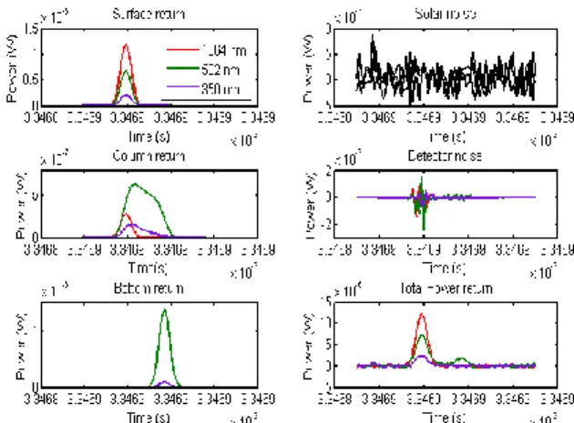
Figure 1 shows simulated waveforms in the case of a satellite LiDAR sensor at an altitude of 500 km, emitting NIR (1064 nm), green (532 nm), and UV (350 nm) wavelengths. Water characteristics used in this simulation correspond to river water conditions with an average turbidity (average concentration of yellow substances ay0 = 0.86 m-1, phytoplankton Cph= 4 mg/m3 and sediment S = 2.8 mg/l) and a 2 m depth. The NIR signal has the highest amplitude from the surface and penetrates a few cm into the water column. The green signal penetrates deeper into the water column and, depending on the water properties, is reflected from the bottom. The UV wavelength penetrates considerably through the water column and can reach the bottom, but the response is very low.
III. COMPARISON OF SIMULATED TO OBSERVED WAVEFORMS
Simulated waveforms are compared with observed LiDAR waveforms to identify the Wa-LiD model behaviour. The available observed data were provided from the satellite GLAS sensor and the airborne HawkEye sensor (© SHOM).
A. Observed waveforms Datasets
Two datasets were available. The first dataset contains waveforms acquired by the Geosciences Laser Altimeter System (GLAS) across the Lake Leman located in Switzerland and France (Lat. 46°26’N and Long. 6°33’E, Figure 2a). Lake Leman is one of the largest lakes in Western Europe with a surface area of 582 km². The maximum length and width of the lake are 73 km and 14 km, respectively. The
relatively flat surfaces and the fact that the lake is not affected by tides make this a good location for validation studies. The GLAS data used in this study are GLA01. The GLA01 data include waveforms echoed from the water surface in NIR (1064 nm). Each waveform was sampled in 544 or 1000 bins of received power in volts at a sampling rate of 1 ns over land area [16]. In this study, two GLAS transects (set of successive shots or footprints) were selected. Waveforms from these two transects do not have saturation problems and are longer than other transects. The first transect was taken on March 4th 2005 with a length of 11.5 km and corresponds to 69 shots; the second transect was taken on June 7th 2006 with a length of 10.5 km and a corresponding 61 shots.
Fig. 1. Simulated LiDAR Waveforms in NIR (1064 nm), green (532 nm), and UV (350 nm). E0=20 mJ, T0=5 ns, θ=0.3°. Water is of average turbidity
(ay0=0.86 m-1, Cph=4 mg/m3, S=2.8 mg/l) with a depth of 2 m.
(a) (b)
Fig. 2. (a) GLAS transects over Leman Lake, (b) HawkEye points across a coastal area in the northern part of Reunion Island.
The second dataset contains waveforms registered by the airborne HawkEye system across a coastal area in the northern part of Reunion Island near le Chaudron (Lat. 20°52’S and Long. 55°30’E, Figure 2b). The HawkEye LiDAR consists of two laser scanners, one green (532 nm) and one infrared (1064 nm) [17]. The infrared laser light is reflected at the water surface whereas the green laser light continues into the water column. The green laser light is reflected at the seabed, and a portion of the reflected light is collected by the receiver.
Table 1 shows the characteristics of the two LiDAR systems, GLAS [16] and HawkEye [7].
B. Simulated waveforms datasets
Table 2 shows the range of water parameters used for these simulations. A range of probable values of water parameters is
used for the simulation because the exact water properties were not precisely known at the time of the survey; in some cases, it was impossible to measure some of the properties, such as water surface roughness. The range of roughness, r, values used are from Beckman and Spizzochino [15]. The range of sediment concentration for coastal areas varies from 2.6 for clear water to 200 mg/l for very turbid water [18]. Here, we used a smaller range (2.6–10 mg/l) corresponding to clear water. In the same way, as sand in this area is black and formed as a result of volcanic activity [19], the selected range of values for bottom reflectance (Table 2) is the same used by Jun et al. [20].
TABLE1
THE GLAS AND HAWKEYE SYSTEMS PARAMETERS USED IN SIMULATIONS Parameters GLAS HawkEye Parameters GLAS HawkEye
λ (nm) 1064 532-1064 ηe 0.8 0.9 H 600 km 200 m ηR 0.5 0.5 E0 (mJ) 75 3 F 1 1 T0 (ns) 5 7 Δλ (nm) 1.2 1 θ (°) 0,3 20 γr 0.1 0.35 AR (m²) 0,8 0,025 B (MHZ) 100 142 FOV (mrad) 5 30 G 3 3 Rλ (A/W) 0.25 0.3 Id (A) 10-10 10-8 TABLE2
RANGE OF ENVIRONMENTAL PARAMETERS USED IN SIMULATIONS Parameters Range Parameters GLAS HawkEye
r [0.1–0.5] 2 atm T 0.64 0.9 S (mg/l) [2.6–10] β(φ) (m-1sr-1) 0.0014 0.0014 Rb [0.05–0.2] Is (w/m²srnm) 0.025 0.025 ks 0.9 nw 1.33 1.33 C. Waveforms comparison
The amplitude of GLAS waveforms is in volts whereas the units for HawkEye are not known because of industrial trade secrets. For the Wa-LiD simulations, the waveforms are expressed in watts. For these reasons as well as the invariant shapes of waveforms and the fact that peaks in waveforms are the main information retrieved, the chosen method to compare simulated and observed waveforms was to compare the signal-to-noise ratio (SNR). Here, SNR is defined by the ratio between the waveform peak amplitude (water surface, bottom) and the standard deviation of detection noise (includes also the photon noise of the useful signal). The distributions of SNR for simulated and observed waveforms were computed. The 95%, 90%, 75% and 50% confidence intervals were thus calculated from SNR quantiles for both observed waveforms (GLAS and HawkEye) and simulated ones. Next, the probabilities for an observed SNR to belong to a given simulated SNR confidence interval were computed. The number of simulated waveforms chosen was around two times higher than the number of observed waveforms to ensure a better simulation of extremes.
D. Results and discussion
1) Comparison with GLAS waveforms
Waveforms were simulated from Wa-LiD using the GLAS system parameters (Table 1) and the range of values for roughness r (Table 2). In the infrared, the waveforms are
influenced mainly by the water surface roughness because the penetration of this wavelength is very low in the water column and the LiDAR return comes primarily from the water surface. In all, 260 waveforms were generated by random, and water surface properties were uniformly selected within the ranges given in Table 2. From the two GLAS transects selected, 130 GLAS waveforms across Leman Lake were used. Next, GLAS and simulated SNR distributions were computed and assigned confidence intervals. The probability of a GLAS SNR (SNRGLAS) value belonging to the simulated SNR
(SNRwalid) confidence intervals is higher (Figure 3a)
(approximately 0.99 at a 95% confidence interval) than the opposite (Figure 3b) (approximately 0.57 at a 95% confidence interval). In the Wa-LiD model, the water surface albedo (Ls)
is influenced by two water surface properties: the specular reflection coefficient and the surface roughness. The underestimation of the simulated SNR is probably due to the distribution of unknown water properties compared with simulations from distributions of uniform water properties.
Fig. 3. a) Probability for an observed SNR to belong to a simulated SNR interval, b) Probability for a simulated SNR to belong to an observed SNR interval.
2) Comparison with HawkEye waveforms
NIR channel
In all, 400 waveforms were simulated from Wa-LiD using the HawkEye system characteristics (Table 1) and a wide range of values for water surface roughness (Table 2). They were compared to 200 observed HawkEye waveforms. The probability of HawkEye SNR (SNRHawk) belonging to
SNRwalid confidence intervals are higher (approximately 0.98
at a 95% confidence interval) than the opposite (approximately 0.66 at a 95% confidence interval) (Figure 3). The weak underestimation of simulated SNR may result for the same reason as the underestimation for GLAS (i.e., unknown values of properties for actual surface water distribution), which may demonstrate the limitations of this comparison exercise. This result confirms the capability of the Wa-LiD model to simulate realistic LiDAR waveforms in the NIR.
Green channel
The simulated waveforms in the green were carried out using the same system parameters as those for the infrared, except for the wavelength value (532 nm). The water parameters (Table 2) were randomly selected as inputs for the simulator. The water surface roughness r has a higher impact on the surface echo, and the sediment concentration S has the higher impact on the water column echo for coastal areas [18].
In contrast, the bottom reflectance Rb has the higher impact on
the bottom echo. The remaining water parameters were fixed for values that belong to clear coastal water (ay0=0.1 m-1,
Cph=1 mg/m3). The comparison between HawkEye and
simulated waveforms were carried out for 4 water depths: 3, 6, 10, and 15 m. For each depth, 400 simulations were generated. For comparison, 94 HawkEye waveforms were used: 21 at 3 m, 20 at 6 m, 20 at 10 m, and 18 at 15 m depths.
HawkEye and simulated data were compared using the SNR for both the surface and bottom returns. The same confidence intervals were calculated for each considered bathymetry. Figure 4 presents the boxplots of SNR for surface and bottom returns from simulated and HawkEye green waveforms at a 3 m depth. There is a high probability (higher than 0.8) that the HawkEye surface SNR (SNRHawk) belong to
the simulated surface SNR 95% confidence interval for all water depths (Figure 3a). These probabilities were higher than those of a simulated surface SNR to belong to the HawkEye surface SNR confidence intervals. At the bottom, the probability of HawkEye SNR (SNRHawk) to belong to the
simulated bottom SNR confidence intervals were slightly higher than the opposite (Figure 3). This weak underestimation of simulated SNR (surface and bottom) is thought to be a result of the unknown actual distribution of 95% at the surface (ks, r), the column (S) and the bottom (Rb),
which does not fully match the distribution of uniform water properties for the simulation.
Fig. 4. Box plots of SNRHawk (surface and bottom) and SNRwalid (surface and
bottom) for HawkEye waveforms in the Green channel at depth of 3 m.
IV. CONCLUSION
A simulation model was built in order to simulate LiDAR waveforms on waters for any emitted wavelength in the optical domain and for different systems characteristics and water properties. The behaviour of the simulator was new explored using datasets of observed waveforms collected from the GLAS satellite sensor over Leman Lake in the NIR channel and from the HawkEye airborne sensor in a coastal area across the northern part of Reunion Island in the NIR and the green channels. The observed and simulated waveforms were analysed by comparing the SNR distribution of their peaks and their confidence intervals, for surface and bottom peaks. The confidence intervals for both observed and simulated SNR are sufficient while presenting some bias, most likely because of the distribution of unknown water properties.
In future works, experiments and research are necessary for a proper characterisation of water surface roughness. Moreover, an analysis of the model sensitivity to different media characteristics and sensor parameters will be carried out to analyse the influential parameters and to assess the performance of future LiDAR systems for the water surface altimetry and bathymetry especially for what concerns the optimisation of the ground processing algorithms.
ACKNOWLEDGMENT
The authors would like to thank the NSIDC (National Snow and Ice Data Centre) and the SHOM (Service Hydrographique et Océanographique de la Marine) for providing GLAS and HawkEye data respectively. The authors are very grateful to EADS (European Aeronautic Defence and Space Company) and CNES (Centre National d’Etudes Spatiales), which both supported this study.
REFERENCES
[1] J. K. Willis, Fu. Lee-Lueng, E. Lindstrom, and M. Srinivasan, "17 years and counting: Satellite altimetry from research to operations,"
Geoscience and Remote Sensing Symposium (IGARSS), 2010 IEEE International, pp.777-780, 2010.
[2] J. L. Irish, and W. J. Lillycrop, “Scanning laser mapping of the coastal zone: the SHOALS system,” ISPRS Journal of Photogrammetry and Remote Sensing, vol. 54, no. 2-3, pp. 123-129, 1999.
[3] D. Feurer, J. S. Bailly, C. Puech, Y. LeCoarer, and A. Viau, “Very high resolution mapping of river immersed topography by remote sensing,”
Progress in Physical Geography, vol. 32, no. 4, pp. 1–17, 2008.
[4] J. S. Bailly, Y. Le Coarer, P. Languille, C. J. Stigermark, and T. Allouis, ”Geostatistical Estimations of bathymetric LIDAR errors on rivers,”
Earth Surface Process and Landforms, vol. 35, pp. 1199-1210, 2010.
[5] G.C. Guenther, “Airborne Laser Hydrography, system design and performance factors,” NOAA Professional Paper Ser. NOS1 (National Oceanic and Atmospheric Administration, Rockville, Md.), 1985. [6] J. Feigels, “LIDARs for oceanological research: criteria for comparison,
main limitations, perspectives,” Ocean Optics XI, vol. 1750, pp. 473– 484, 1992.
[7] H. M. Tulldahl and K. O. Steinvall, “Simulation of sea surface wave influence on small target detection with airborne laser depth sounding,”
Applied Optics, vol. 42, no. 12, pp. 2462 – 2483, 2004.
[8] A. Collin, P. Archambault and B. Long, “Mapping the shallow water seabed habitat with the shoals,” IEEE Transactions on Geoscience and
Remote Sensing, vol. 46, no. 10, pp. 2947-2955, 2010.
[9] N. Baghdadi, N. Lemarquand, H. Abdallah, and J. S. Bailly, “The relevance of GLAS/ ICESat elevation data for the monitoring of river networks,” Remote Sensing, vol. 3, pp. 708–720, 2011.
[10] J. W. McLean, “Modeling of ocean wave effects for lidar remote sensing,” Ocean Optics X, R. W. Spinrad, ed., Proc, vol. 1302, pp. 480– 491, 1990.
[11] R. L. Cook, and K. E. Torrance, “A Reflectance Model for Computer Graphics,” ACM Transactions on Graphics, vol.1, pp. 7 – 24, 1982. [12] A. Bricaud, A. Morel and L. Prieur, “Absorption by dissolved organic
matter of the sea (yellow substance) in the UV and visible domains,”
Limnology and Oceanography, vol. 26, no. 1, pp. 43-53, 1981.
[13] C. D. Mobley, Light and Water: Radiative Transfer in Natural Waters, Academic, San Diego, Calif, 1994.
[14] B. Jutzi, and U. Stilla, “Range determination with waveform recording laser systems using a Wiener Filter,” ISPRS Journal of Photogrammetry
and Remote Sensing, vol. 61, no. 2, pp. 95–107, 2006.
[15] P. Beckmann, and A. Spizzochino, The scatter of electromagnetic waves
from rough Surfaces, Norwood, MA: Artech House, 1987.
[16] H. J. Zwally, B. Schutz, W. Abdalati, J. Abshire, C. Bentley, A. Brenner, J. Bufton, J. Dezio, D. Hancock, D. Harding, T. Herring, B. Minster, K. Quinn, S. Palm, J. Spinhirne, and R. Thomas, “ICESat’s laser measurements of polar ice, atmosphere, ocean, and land,” Journal of Geodynamics, vol. 34, no. 3-4, pp. 405-445, 2002.
[17] A. Wehr and U. Lohr, “Airborne laser scanning-an introduction and overview,” ISPRS Journal of Photogrammetry and Remote Sensing, vol. 54, no. 1-2, pp. 68–82, 1999.
[18] J. A. Warrick, L. A. K. Mertes, D. A. Siegel, and C. Mackenzie, “Estimating suspended sediment concentrations in turbid coastal waters of the Santa Barbara Channel with SeaWiFS” International Journal of Remote Sensing, vol. 25, pp. 1995-2002, 2004.
[19] D. Lorion, “Endiguements et risques d’inondation en milieu tropical. L'exemple de l'île de la Réunion,” Norois, vol. 201, no. 4, pp. 45-66, 2006.
[20] B. Jun, K. Gotoh, H., Kitamura, and H. Koh, “Influence of phytoplankton pigments and bottom features for water quality and depth estimation,” Geoscience and Remote Sensing Symposium, vol. 2, pp. 488-490, 1993.