HAL Id: hal-00180616
https://hal.archives-ouvertes.fr/hal-00180616
Submitted on 20 Oct 2007HAL is a multi-disciplinary open access
archive for the deposit and dissemination of sci-entific research documents, whether they are pub-lished or not. The documents may come from
L’archive ouverte pluridisciplinaire HAL, est destinée au dépôt et à la diffusion de documents scientifiques de niveau recherche, publiés ou non, émanant des établissements d’enseignement et de
Discrete bisector function and Euclidean skeleton in 2D
and 3D
Michel Couprie, David Coeurjolly, Rita Zrour
To cite this version:
Michel Couprie, David Coeurjolly, Rita Zrour. Discrete bisector function and Euclidean skele-ton in 2D and 3D. Image and Vision Computing, Elsevier, 2007, 25 (10), pp.1519-1556. �10.1016/j.imavis.2006.06.020�. �hal-00180616�
Discrete bisector function and Euclidean
skeleton in 2D and 3D
Michel Couprie
(a), David Coeurjolly
(b)and Rita Zrour
(c)(a) Institut Gaspard-Monge, Laboratoire A2SI, Groupe ESIEE, BP99, 93162 Noisy-le-Grand cedex, France. (b) LIRIS, CNRS, 3 boulevard du 11 novembre
1918, 69622 Villeurbanne cedex, France. (c) LLAIC, B.P. 86, 63172 Aubiere cedex, France.
Abstract
We propose a new definition and an algorithm for the discrete bisector function, which is an important tool for analyzing and filtering Euclidean skeletons. We also introduce a new thinning algorithm which produces homotopic discrete Euclidean skeletons. These algorithms, which are valid both in 2D and 3D, are integrated in a skeletonization method which is based on exact transformations, allows the filtering of skeletons, and is computationally efficient.
Key words: Bisector function, skeleton, Euclidean distance transform, Voronoi diagram, digital topology
1 Introduction
The notion of skeleton, or medial axis, plays a major role in shape analy-sis. It has been introduced by Blum [5] and is the subject of an abundant literature, which deals with both metrical and topological aspects, and rests on different approaches, in particular discrete geometry [6,14,19,25], digital topology [13,17,18], mathematical morphology [32,34], computational geom-etry [1,2], and partial differential equations [30]. In this paper, we focus on skeletons in the discrete grid Z2 or Z3, which are centered in the shape with respect to the Euclidean distance, and which have the same topology as the original shape.
Email addresses: [email protected] (Michel Couprie), [email protected] (David Coeurjolly), [email protected] (Rita Zrour).
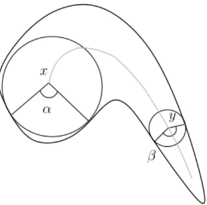
x
y α
β
Fig. 1. Illustration of the bisector function θ. In this example, θ(x) is the angle α, and θ(y) is the angle β.
Introduced by Meyer [23], and further studied by Talbot and Vincent [32], the bisector function can play an important role in analyzing and filtering skeletons [1,2,19]. Informally, the bisector function associates to each object point x the maximal angle formed by x (as the vertex) and the points of the background which are nearest to x (see Fig. 1). Until now, the algorithms proposed to compute the bisector function in Z2 were based on the use of
vectors produced by distance transformation algorithms (e.g., [9]). To each object point, with such algorithms, only one vector indicates the location of a closest background point, and some other points at the same distance may be ignored.
The medial axis of an object X is composed by the centers of the balls which are included in X but which are not included in any other ball included in X. This set of points is, by nature, centered in the object with respect to the dis-tance which is used to define the notion of ball. In discrete spaces, the medial axis has not, in general, the same topology as the original object. The use of guided and constrained discrete homotopic transformations has been proposed by several authors to obtain an homotopic skeleton which contains the medial axis (see [13] which is, to our best knowledge, the first paper presenting this approach). Among them, Talbot and Vincent [32] propose an algorithm for the 2D case which guarantees that the skeleton branches follow lines of steepest slope of the Euclidean distance map of the object, a property which is veri-fied in the continuous framework. This algorithm cannot be straightforwadly extended to the 3D case.
This paper contains two original contributions. First, we propose a new def-inition and an algorithm to compute a discrete bisector function in 2D or 3D spaces. This algorithm is based on an optimal procedure for building a complete discrete Voronoi diagram of a shape. Second, we introduce a new thinning method which produces homotopic discrete Euclidean skeletons. Un-like previously proposed approaches, this method is also valid in 3D.
Using these two original algorithms, we propose an integrated skeletonization method for objects in Z2 and Z3 which is based on exact discrete metrical
and topological transformations, allows the filtering of the skeleton under the control of two parameters, and is computationnaly efficient.
2 Basic notions
In this section, we recall some basic metrical and topological notions for binary images [11,17]. For the sake of simplicity, we limit this presentation to the 2D case.
We denote by Z the set of integers, by N the set of nonnegative integers, and by N∗
the set of strictly positive integers. We denote by E the discrete plane Z2. A point x in E is defined by (x
1, x2) with xi in Z. Let x, y ∈
E, we denote by d2(x, y) the square of the Euclidean distance between x
and y, that is, d2(x, y) = (x
1 − y1)2 + (x2 − y2)2. Let Y ⊂ E, we denote
by d2(x, Y ) the square of the Euclidean distance between x and the set Y ,
that is, d2(x, Y ) = min{d2(x, y); y ∈ Y }. Let X ⊂ E (the “object”), we
denote by D2
X the map from E to N which associates, to each point x of E,
the value D2
X(x) = d2(x, X), where X denotes the complementary of X (the
“background”). The map D2
X is called the (squared Euclidean) distance map
of X. Let x ∈ E, r ∈ N∗
, we denote by Br(x) the ball of (squared) radius r
centered on x, defined by Br(x) ={y ∈ E, d2(x, y) < r}. Notice that, for any
point x in X, the value D2
X(x) is precisely the radius of a ball centered on x
and included in X, which is not included in any other ball centered on x and included in X.
Let us recall the notion of medial axis (see also [26,32]). Let X ⊆ E, x ∈ X, r∈ N∗
. A ball Br(x)⊆ X is maximal for X if it is not strictly included in any
other ball included in X. The medial axis of X, denoted by MA(X), is the set of the centers of all the maximal balls for X (see Fig. 2d, see also Fig. 3). In the framework of mathematical morphology, an alternative definition of the medial axis in terms of openings has been introduced by Lantuejoul [31].
Efficient algorithms have been proposed to compute exact squared Euclidean distance maps [28,16,22], and also to extract the exact Euclidean medial axis of a shape, from an exact squared Euclidean distance map and using pre-computed look-up tables [6,25]. An optimal, linear-time algorithm has been proposed by one of the authors to extract a subset of the medial axis which is sufficient to reconstruct the original shape [8].
In discrete spaces, it is well known that the topology of the medial axis is generally not the same as the topology of the original object. In particular,
if X is connected, MA(X) is generally not connected (see Fig. 2d). Let us now introduce some topological notions in Z2 that we use in the sequel.
We consider the two adjacency relations Γ4 and Γ8 defined by, for each
point x ∈ E: Γ4(x) = {y ∈ E; |y1 − x1| + |y2 − x2| ≤ 1}, Γ8(x) =
{y ∈ E; max(|y1 − x1|, |y2 − x2|) ≤ 1}. In the following, we will denote
by n a number such that n = 4 or n = 8. We define Γ∗
n(x) = Γn(x)\ {x}. The
point y∈ E is n-adjacent to x ∈ E if y ∈ Γ∗
n(x); it is n-adjacent to a subset X
of E if it is n-adjacent to at least one point of X. An n-path is a sequence of points x0. . . xk with xi n-adjacent to xi−1 for i = 1 . . . k.
Let X be a nonempty subset of E. We say that two points x, y of X are n-connected in X if there is an n-path in X between these two points. This defines an equivalence relation. The equivalence classes for this relation are the n-connected components of X, or n-components in short. The set X is said to be n-connected if it consists of exactly one n-component. The set composed of all n-components of X which are n-adjacent to a point x is denoted by Cn[x, X].
In order to have a correspondence between the topology of X and the topology of X, we have to consider two different kinds of adjacency for X and X [17]: if we use the n-adjacency for X, we must use the n-adjacency for X, with (n, n) = (8, 4) or (4, 8). In the sequel, we assume that the adjacency pair (n, n) = (8, 4) has been chosen and we do not write the subscripts n, n unless necessary; but the results also hold for (n, n) = (4, 8).
Informally, a simple point p of a discrete object X is a point which is “inessen-tial” to the topology of X [27]. In other words, we can remove the point p from X without “changing the topology of X”. The notion of simple point is fundamental to the definition of topology-preserving transformations in dis-crete spaces. We now give a definition and a local characterization of simple points in E = Z2. For the 3D case, see [4].
The point x∈ X is simple (for X) if each n-component of X contains exactly one n-component of X \ {x} and if each n-component of X ∪ {x} contains exactly one n-component of X. Let X ⊆ E and x ∈ E, the two connectivity numbers [4] are defined as follows (#X stands for the cardinality of X):
T (x, X) = #Cn[x, Γ∗8(x)∩ X]; T (x, X) = #Cn[x, Γ∗8(x)∩ X].
The following property allows us to locally characterize simple points [17,4], hence to implement efficiently topology preserving operators:
x∈ E is simple for X ⊆ E ⇔ T (x, X) = 1 and T (x, X) = 1.
Let X be any finite subset of E. The subset Y of E is an homotopic thinning of X if Y = X or if Y may be obtained from X by iterative deletion of simple points. We say that Y is an ultimate homotopic skeleton of X if Y is an homotopic thinning of X and if there is no simple point for Y .
constrained by C if C ⊆ Y , if Y is an homotopic thinning of X and if there is no simple point for Y in Y \ C (see e.g. [13,34]). The set C is called the constraint set relative to this skeleton.
(a) (b) (c) (d) (e)
Fig. 2. (a): a set X (in white); (b): an homotopic thinning of X; (c): ultimate homotopic skeleton of X; (d): medial axis of X, computed by the algorithm of [25]; (e): ultimate homotopic skeleton of X constrained by the medial axis of X. In (b,c,d,e) the original set X appears in gray for comparison.
3 Complete discrete Voronoi mapping
In order to compute the bisector function, we need to know for each shape point x the set of background points which are at minimal distance from x. We propose in this section an optimal algorithm to compute these sets, based on the notion of Voronoi diagram.
3.1 Preliminaries
We first remind the definition of the Voronoi diagram in the continuous plane.
Given a set S = {si} of points or sites in R2, the Voronoi diagram of S is
a decomposition of the plane into a set of cells C = {ci} (one cell ci ⊂ R2
per site si) such that for each point p in the (open) cell ci, we have d(p, si) <
d(p, sj) for any j 6= i. In other words, any p in ci is closer to the site si
than to any other site sj [24]. We also consider the closed cells defined by
c−
i = {p ∈ R2; d(p, si) ≤ d(p, sj)}. The cell boundaries correspond to loci of
points equidistant to two or more sites.
In the discrete plane, we can define a Voronoi labeling by assigning to each grid point the index of a Voronoi cell containing it. For grid points which are situated on the boundaries of the Voronoi diagram, the index of one of the neighboring cells is chosen arbitrarily. Based on this definition, algorithms can be designed to construct such a Voronoi labeling considering an error-free Euclidean metric, see [7,21,15]. To summarize the contributions of these authors, the Voronoi labeling can be computed in linear time with respect
to the number of grid points whatever the dimension of the image. However, the main drawback of these approaches lies in the arbitrary choices which are made for cell boundary points which coincide with discrete points, making the Voronoi labeling not unique.
To overcome this drawback, we propose to use the Voronoi mapping defined below (also called feature transform in [15]) instead of the Voronoi labeling.
LetE be either R2 or Z2, let S be a nonempty subset of E, and let x ∈ E. The
projection of x on S, denoted by ΠS(x), is the set of points y of S which are
at minimal distance from x; more precisely, ΠS(x) = {y ∈ S, ∀z ∈ S, d(y, x) ≤
d(z, x)}. For example in Fig. 3a, we have ΠX(x) = {a, b} and ΠX(y) = {c}, and in Fig. 3b, we have ΠX(x) = {a} and ΠX(y) ={b, c}.
We can see that a point p belongs to the closed cell c−
i (using the above
nota-tions for the Voronoi diagram) if and only if the site sibelongs to the projection
ΠS(p). Hence, we call Voronoi mapping the map ΠS which associates, to each
point p ofE, the set ΠS(p).
x y c a b θ x y z b c a e d q p (a) (b)
Fig. 3. (a): A subset X of the continuous plane (full ellipse, represented by its border) and its medial axis (horizontal line segment), a point x and its projection {a, b} on X, a point y and its projection {c}. Notice that y does not belong to the medial axis, since no ball centered on y and included in X is maximal for X (the ball with dashed contour contains them all). (b): A subset X of the discrete plane (represented by white dots), its complementary X (black dots) and the continuous Voronoi diagram associated to X (the gray lines represent the Voronoi boundaries). The projection of x (resp. y, z) on X is the set {a} (resp. {b, c}, {c}). See Sec. 4.1 for the use of p, q, e, and d.
A naive computation of the Voronoi mapping can be sketched as follows: first we construct the complete Euclidean Voronoi diagram using an algorithm from Computational Geometry [24] using points in X as sites. Then, we can digitize the Voronoi diagram to obtain the Voronoi mapping: for each point x∈ X, we locate the closed cell c−
i such that x∈ c −
i in order to define ΠX(x). Although,
points in X and n′
the number of points in X, the overall computational cost would be O(n′log n′ + n log n′) (for the 2D case; things get worse in higher
dimensions). Indeed, this algorithm does not take into account the specific regularity of the sets X and X.
In the next section, we sketch an optimal algorithm to compute the Voronoi mapping from an error-free Euclidean metric using specific features of the discrete grid.
3.2 Voronoi mapping computation
We modify the Voronoi labeling algorithm proposed in [15]1. This algorithm
is based on separable techniques to compute the exact squared Euclidean distance transform (SEDT) [28,16,22], the reverse EDT or the medial axis [8].
We first present here the SEDT algorithm in the 2D case: we consider a two-dimensional binary image F ={fij} in the form of a boolean array of width w
and height h, and we set n = w×h. We denote by X the set {(i, j), fij = 1} of
“object” points. The output of the algorithm is a 2D image H ={hij} storing
the squared distance transform. The SEDT algorithm consists of the following steps.
(1) Build from the source image F a one-dimensional SEDT according to the first dimension (i−axis), denoted by G = {gij}, where, for a given row j:
gij = min
(u,j)∈X{(i − u)
2} . (1)
(2) Then, construct the image H ={hij} with a j−axis process:
hij = min
v {giv+ (j− v)
2, 1≤ v ≤ h} . (2)
To transform this SEDT algorithm in order to produce an error-free Voronoi labeling, we just have to mark one of the points in X that lead to the mini-mum distance [28,22]. To maintain the complete list of projected points when #ΠX(x) > 1, we propose a separable technique that constructs the error-free Voronoi mapping dimension after dimension.
First, we can easily modify the step 1 of the previous SEDT algorithm to associate to each point of x ∈ X, its projection according to the i−axis (i.e. the set of points of X on the same row as x which are at minimal distance from x). Since the step 1 of the SEDT algorithm requires O(n) computation
1 An implementation of this algorithm is available in dimension 3 at the web page:
steps, the 1D Voronoi mapping according to the i−axis can also be computed in O(n).
The second step can be viewed as a lower envelope computation of a set of parabolas in each column [28,16,22] (see graphs on the right of Fig. 4). During this lower envelope computation, we can maintain the Voronoi mapping with the following observations related to the sweep line techniques to construct the (continuous) Voronoi diagram in computational geometry [3]. Let us consider the 1D Voronoi mapping Π computed after the step 1, and a point x ∈ X such that #Π(x) > 1 (i.e. x is on a boundary of the 1D Voronoi diagram):
(1) the Voronoi diagram boundary at x may disappear, in that case, the new projection of x may be reduced to one point ;
(2) the Voronoi diagram boundary at x may be preserved, in that case the new projection of x contains the equidistant sites detected along the i−axis ;
(3) new equidistant points in X can be detected when two parabolas of the lower envelope intersect in x. Hence, new points may be inserted in Π(x) (see Fig. 4).
We do not detail here the overall algorithm but the Voronoi mapping can computed in O(n′
+ m) where m = Px∈X#ΠX(x) and n ′
is the number of points of F which are not in X (background points). Since the size of the memory space needed to store the projection sets is in O(m), this algorithm is optimal both in space and time complexity. Furthermore, the experiments reported in Annex A show that m is usually close to the number of image object points, especially in 2D.
In three dimensions, we use the same decomposition as proposed to solve the SEDT problem: we just have to add a new lower envelope computation according to the third axis. The above observations are still valid and we also obtain an O(n′
+ m) algorithm to extract the Voronoi mapping (where n′
and m are defined as above). The method extends to higher dimensions as well.
4 Bisector function
The bisector angle of a point x in X can be defined, in the continuous frame-work, as the maximal unsigned angle formed by x (as the vertex) and any two points in the projection of x on X [23,32]. In particular, if #ΠX(x) = 1, then the bisector angle of x is zero. For example in Fig. 3a, the bisector angle of x is θ, and the bisector angle of y is 0. The bisector function of X is the function which associates to each point x of X, its bisector angle in X.
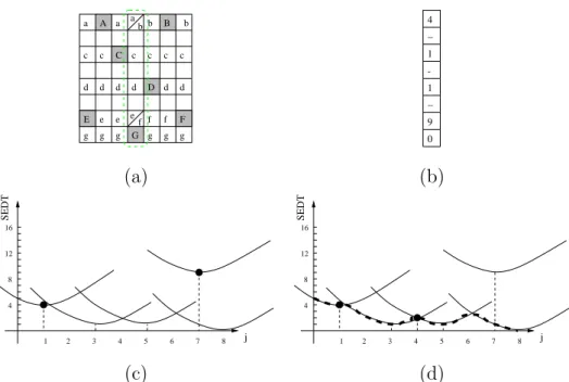
G D F E A B C a a b b c c c d d d e e g g g g g f f e b a f g c c c d d d 4 1 1 9 0 -− − (a) (b) SEDT 4 8 12 1 2 3 16 4 5 6 7 8 j SEDT 4 8 12 1 2 3 16 4 5 6 7 8 j (c) (d)
Fig. 4. Illustration of the dimensional decomposition of both the SEDT algorithm and the Voronoi mapping. (a): An input image (pixels of X are in gray), with the Voronoi mapping according to the i−axis (e.g., the letter a denotes a reference to point A of X, etc). (b): the SEDT of the column i = 4. (c): The set of parabola associated to this column, black dots indicate points x such as #Π(x) > 1 detected during the first (horizontal) process. (d): The final lower envelope of the set of parabolas (bold dashed line) and the final set of points x with #Π(x) > 1: the point j = 7 has disappeared (case (1)), the point j = 1 has been preserved (case (2)), and a new Voronoi diagram boundary has appeared for j = 4 (case (3)) in the Voronoi mapping.
This very definition of the bisector function was used in [2] in order to provide a filtering criterion for skeletons based on Voronoi diagrams in the continuous plane. It has been also adapted to the discrete case in [32,19]. The main drawback of the latter approaches is to use a non-unique Voronoi labeling in which only one site of the entire set of the equidistant sites is considered.
4.1 Extended projection
A direct extension of the above definition to the discrete case does not lead to a satisfactory notion of bisector function, in particular with respect to our goal of filtering the medial axis. Consider the set X in Fig. 3b, symbolized by the white dots. We can see that the point x of X belongs to the (discrete) medial axis of X, as defined in Sec. 2. The projection ΠX(x) is {a}, thus the bisector angle of x according to the previous definition is zero. On the other hand, in the neighborhood of x there exists a (non-grid) point p on the Voronoi boundaries which has a bisector angle of π. In order to preserve
this information, we would like that the value of the bisector angle associated with x be π rather than 0. Similarly, for the point y we would like to have a bisector angle greater than byc, due to the existence in the closed unit squared centered on y, of a point q having a bisector angle equal to bqe. This informald discussion motivates the following definition of the extended projection and of the discrete bisector function.
Definition 1. Let X ⊂ E, and let x ∈ X. The extended projection of x on X, denoted by Πe
X(x), is the union of the sets ΠX(y), for all y in Γ4(x) such that
d2(y, X)≤ d2(x, X).
Let X ⊂ E, and let x ∈ X. The (discrete) bisector angle of x in X, denoted by θX(x), is the maximal unsigned angle between the vectors
→
xy,xz, for all y, z→ in Πe
X(x). In particular, if #Π e
X(x) = 1, then θX(x) = 0. The (discrete)
bisector function of X, denoted by θX, is the function which associates to each
point x of X, its discrete bisector angle in X.
With this definition, we can easily check that the bisector angle of the point x in Fig. 3b is equal to π; and that θX(y) =bye, a value close tod bqe.d
Let us explain the role of the condition d2(y, X) ≤ d2(x, X) (1) in our
defi-nition of the extended projection. Consider the situation depicted in Fig. 5a, where a Voronoi boundary (bold line) separates the two object points x and y. A background point a (resp. b) in the projection of x (resp. y) is depicted. Observe that x is closer to X than y. Without condition (1), the extended projection of x would contain b and the extended projection of y would con-tain a. With condition (1), we have a∈ Πe
X(y) but b /∈ Π e
X(x). In other words,
with condition (1) only y receives a high bisector angle value, while without condition (1) both x and y receive high bisector angle values. Fig. 5b and Fig. 5c show details of a bisector function computed without (1) and with (1) respectively, on the same object. For filtering purposes, Fig. 5c is clearly a better result.
Thanks to the algorithm presented in Sec. 3.2, the Voronoi mapping ΠX can be computed in optimal time. For each object point x, we must then compute Πe
X(x) using the adjacency relation Γ and the distance map D 2
X. The last
step to obtain the bisector angle consists in the computation of the maximum unsigned angle between all the pairs of vectors{xy,→ xz→} for all y, z in Πe
X(x).
If we denote by k the number of points in Πe
X(x), the number of such pairs
is quadratic with respect to k, more precisely, it is equal to k(k− 1)/2. By normalizing all these vectors, we can easily see that the problem of finding a maximum angle reduces to the problem of finding a maximum diameter of a convex polygon in 2D. This last problem has been solved in 1978 by Shamos [29], who provided a simple linear-time algorithm (that is, in O(k)). In 3D, the problem is more complicated but some efficient algorithms (in
x a y b 5 178 180 178 5 6 0 6 6 7 5 0179 179 0 5 6 6 6 0 6 5178 180 178 5 6 14 14 15 6 5 0 179 17913 13 14 14 15 0 0 0 177 17512 13 0 0 0 0 0 0 0 177 1790 8 8 8 0 0 0 0 179 1777 8 8 8 0 0 0 8 179 180 179 8 0 0 9 8 8 8 7177 179 0 8 8 9 8 8 8 0179 177 7 8 21 9 0 0 0 0179 180 17920 13 0 0 0 0 0 0 176 17512 13 0 0 0 0 0 0 177 1780 0 0 0 0 0 0 0 178 1770 0 0 0 0 0 13 12175 17616 17 5 5 180 5 5 6 0 0 6 7 0 0 179 1790 0 6 6 6 0 6 5 5 180 5 5 6 0 0 15 6 0 0 179 1790 13 14 14 15 0 0 0 017512 13 0 0 0 0 0 0 0177 0 0 0 0 8 0 0 0 0 0 177 7 8 8 8 0 0 0 8 7 180 7 8 0 0 9 8 8 8 7 177 0 0 0 0 9 8 0 0 0 0 177 7 8 8 0 0 0 0 0 0 180 7 20 13 0 0 0 0 0 0 17312 12 13 0 0 0 0 0 0 177 0 0 0 0 0 0 0 0 0 0177 0 0 0 0 0 0 13 12 12173 0 0 (a) (b) (c)
Fig. 5. (a): illustration of the role of condition (1); (b): detail of a bisector function computed without condition (1); (c): detail of a bisector function computed with condition (1). Angle values are in degrees.
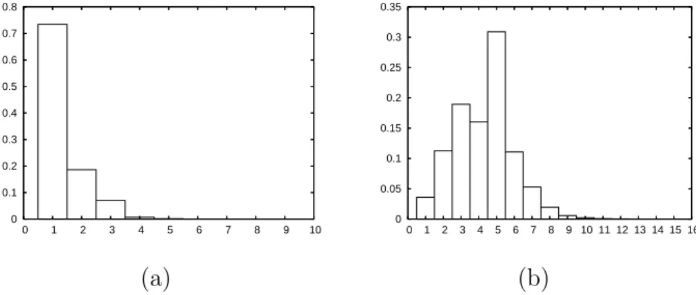
O(k log k) or less) have been proposed for the maximal diameter of a set of points, see e.g. [20]. However, in practice, the mean cardinal of the extended projections for a given shape is usually quite small. For example, it is close to 1.7 for the 2D object of Fig. 7, and close to 4.3 for the 3D object of Fig. 9. In Annex B, we show the distribution of #ΠX(x) and #Πe
X(x) for these objects.
If we consider only the extended projection of medial axis points, the mean values are respectively of 2 and 4.5. Thus, the straightforward algorithm which considers all the pairs of points in the extended projection is the best choice in most cases.
(a) (b) (c) (d)
Fig. 6. (a): a set X and its medial axis [25] (in black); (b): the bisector function θX
(dark colors correspond to wide angles); (c): filtered medial axis, based on the values of θX; (d): detail of the non-filtered and filtered medial axis.
In Fig. 6, we show a set X together with its medial axis (a) and the discrete bisector function θX (b). We illustrate the use of this function to eliminate
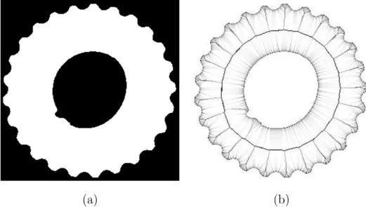
spurious points of the medial axis: in (c), we show the points of the medial axis (in black) which have a bisector angle greater than 40 degrees. A zoomed detail of both axes is shown in (d). Notice that only the bisector angles of the medial axis points need to be computed for this application. Fig. 7 shows the bisector function of a more complex 2D shape.
(a) (b)
Fig. 7. (a): a set X (in white); (b): the bisector function of X.
Let us analyse the differences between the Talbot’s discrete bisector func-tion [33] and ours. Let X ⊂ E, x ∈ X, and let V (x) denote a point arbitrarily chosen in ΠX(x). We set B(x) = max{angle(y1→z1,
→
y2z2), y1 ∈ Γ4(x), y2 ∈
Γ4(x), z1 = V (y1), z2 = V (y2)} (notice that the definition of Talbot is
re-stricted to the points of the skeleton, and corresponds actually to B(x)/2). A first difference lies in the arbitrary choices done by the algorithm which finds a closest background point for each object point, formalized here by the notation V (x). In our case, all the points of ΠX(x) are considered, thus no choice is done.
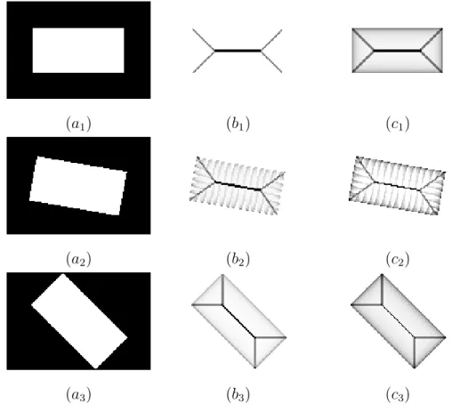
Fig. 8 illustrates a second difference. Observe that depending on the contour orientation, (e.g., horizontal, vertical or diagonal) Talbot’s bisector angles can be very different, even for points which are not located on the contour. On the other hand, our definition and algorithm provide a more homogeneous result, whatever the contour orientation (see also Fig. 7). This is due to the choice of considering the point x itself as the only vertex for all the angles which are considered to compute θX(x). On the other hand, the definition of B(x)
is based on angles with different vertices in Γ4(x).
The definition and computation of this discrete bisector function can be straightforwardly extended to Z3. To conclude this section, we present in
Fig. 9 an illustration of the bisector function of a three-dimensional object (a vertebra).
(a1) (b1) (c1)
(a2) (b2) (c2)
(a3) (b3) (c3)
Fig. 8. (a1, a2, a3): a set X (in white); (b1, b2, b3): Talbot’s bisector function;
(c1, c2, c3): our bisector function.
5 New distance-guided homotopic thinning algorithm
The skeletonization methods which are based on homotopic thinnings, in the sense of section 2, provide a formal guarantee that the skeleton and the orig-inal object have the same topology. The simplest such method consists in computing an ultimate homotopic skeleton of the object X constrained by the medial axis of X, that is, removing iteratively simple points from X which do not belong to MA(X), taking the distance map as a priority function in order to select first the points which are closest to the background. This can be done using the following procedure, with P = DX and Y = MA(X).
Procedure UltimateSkeleton (Input X, P , Y , Output Z) 01. Z ← X
02. Q ← {(P (x), x); where x is any point of X \ Y } 03. While Q6= ∅ Do
04. choose (p, x) in Q such that p is minimal; Q ← Q \ {(p, x)} 05. If x is simple for Z Then
06. Z ← Z \ {x}
(a) (b)
(c) (d)
Fig. 9. (a): a view of a subset X of Z3 (vertebra), generated thanks to a
topolog-ically sound “Marching Cubes-like” algorithm [10]; (b,c,d): the bisector function, illustrated in an “X-ray” manner: the gray level of a point corresponds to the aver-age of the bisector angles on a straight line parallel to one of the three axes.
The drawback of this method has been well analyzed in [32]. Roughly speaking the method does not guarantee that points of the homotopic skeleton outside the medial axis are “well centered” in the object; more precisely, such a point may have a null or quasi-null bisector angle.
Let us consider the object X in Fig. 10a, and the constraint set Y in Fig. 10c, which consists of the four corner points of the shape. The result of UltimateSkeleton(X, DX, Y ) is depicted in Fig. 10d. The isolines of the
distance map DX and the bisector function of X are depicted in Fig. 10b,e
respectively, for comparison.
To understand what happens, let us concentrate on a detail of the above example, depicted in Fig. 11. The numbers correspond to the distance map values. The circled point with value 1 is one of the points belonging to the constraint set Y . Suppose that all the points with a value below 8 have been
(a) (b) (c) (d) (e) (f)
Fig. 10. (a): a set X (in black); (b): isolines of the Euclidean map DX; (c): a
constraint set Y (four points located at the “corners” of the shape); (d): homotopic skeleton of X guided by D2
X and constrained by Y ; (e): the bisector function of X;
(f): the result of our algorithm EuclideanSkeleton.
25 16 9 25 16 9 18 8 13 8 5 8 5 2 13 0 1 4 0 1 4 0 1 4 0 1 2 0 0 1 v w z
Fig. 11. A detail of the preceding example.
processed by the homotopic thinning algorithm. At this step, the points in gray are still in X, as well as the two circled points (the point at 1 because it belongs to Y , and the one at 4 because it is not a simple point). All other points are not in X. Obviously, the point v at 8 adjacent to z at 4 will be selected before its neighbor w at 9, and since it will be a simple point at this stage, it will be deleted. Such a behaviour will be reproduced at later stages, generating a diagonal branch of the skeleton, and is in contradiction with a property of the skeleton in the continuous framework: informally, skeleton branches follow lines of steepest slope of the Euclidean distance map. Let us compute the slopes of zv and zw in our example: (√8−√4)/1 ≈ 0.83, and (√9−√4)/√2≈ 0.71. Thus, the point v should be kept in the skeleton and the point w deleted according to this criterion.
In [32], Talbot and Vincent propose the following strategy to cope with this problem. During the thinning process guided by the distance map, having de-tected a point x which belongs to the skeleton (either a point of the constraint set or a non-simple point), the neighbor of x which corresponds to the steep-est ascending slope is dynamically added to the constraint set. Although this method gives satisfactory results in 2D, it cannot be extended to the 3D case.
We propose another strategy which gives equivalent results in 2D and which also applies to the 3D case. The idea is to define a priority function which takes into account both the distance map and an auxiliary function defined in the neighborhood of each dynamically detected skeleton point. Let x be such a
point, then to any neighbor y of x which is still in X and not in the constraint set Y , we associate the value py = DX(x) + (DX(y)− DX(x))/d(x, y), with
DX(x) = q
D2
X(x). The new priority function, for the point y, is defined as
min(py, DX(y)). We see that (DX(y)− DX(x))/d(x, y) is the slope of xy, thus
the neighbors of x will be examined in increasing order of slope, since the value py is always less or equal to the corresponding distance value DX(y) (for
all x, y in Z2 or Z3 with x6= y, we have d(x, y) ≥ 1).
For example, in the above situation, we have DX(v) =
√ 8≈ 2.83, DX(w) = 3, pv = √ 4 + (√8−√4)/1 = √8 and pw = √ 4 + (√9−√4)/√2 ≈ 2.71; thus the point w will be selected before v with this strategy. Our algorithm is given below.
Procedure EuclideanSkeleton (Input X, DX, Y , Output Z)
01. Z ← X
02. Q ← {(DX(x), x); where x is any point of X\ Y }
03. R ← {(px, x); where x is any point of X \ Y adjacent to Y ,
04. and where px = min{DX(z) + (DX(x)− DX(z))/d(x, z), z ∈ Y } } 05. While Q6= ∅ Or R 6= ∅ Do
06. choose (p, x) in Q∪ R such that p is minimal 07. Q ← Q \ {(p, x)}; R ← R \ {(p, x)}
08. If x∈ Z \ Y Then
09. If x is simple for Z Then 10. Z ← Z \ {x}
11. Else
12. Y ← Y ∪ {x}
13. R ← R ∪ {(py, y); where y ∈ Γ(x) ∩ (Z \ Y )
14. and where py = DX(x) + (DX(y)− DX(x))/d(x, y)}
In Fig. 10f, we see the result of this algorithm applied to the preceding exam-ple. Compare the shape of this skeleton with the distance map and with the bisector function of X depicted in 10b,e respectively. Note that, depending on the choice of the couple (p, x) in the case of equal priorities (line 6), different results may be obtained. The complexity of this algorithm depends on the data structure used to represent the sets Q and R. To be more precise, this data structure must allow to perform the choice in line 6 efficiently, and also the insertions in lines 12 and 13. Using for example balanced binary trees [12], the overall complexity of the algorithm is in O(n log n), where n is the number of image points.
6 Filtered Euclidean skeletons in 2D and 3D
In [2], Attali and Montanvert show that an efficient filtering of a skeleton can be performed by removing two kinds of medial axis points: those which correspond to maximal balls of small radius, and those which have a small bisector angle (see also [1]).
Based on the methods described in the previous sections, we propose a parame-trized filtered Euclidean skeleton procedure which has the following qualities: - flexible (it allows the removal of unwanted skeleton parts under the control of two parameters),
- general (it applies to 2D and 3D objects with arbitrary topology),
- based on well-defined notions (distance transform, medial axis and discrete bisector function), - topologically sound (topology preservation is guaranteed by the use of homotopic transformations),
- efficient in terms of processing speed.
Procedure FilteredSkeleton (Input X, r, α, Output Z) 01. D2 X ← SEDT(X) 02. M ← MedialAxis(X, D2 X) 03. Z ← EuclideanSkeleton(X, D2 X, M ) 04. θX ← DiscreteBisector(X, M) 05. Y ← {x ∈ M; D2 X(x)≥ r2 and θX(x)≥ α} 06. Z ← UltimateSkeleton(Z, D2 X, Y )
The exact squared Euclidean distance transform (SEDT) may be computed in linear time, both in 2D and 3D, see [28,16,22] and Sec. 3.2. It only has to be computed once and is used by procedures MedialAxis, EuclideanSkele-ton and UltimateSkeleton. Procedure MedialAxis can be efficiently im-plemented in 2D and 3D thanks to the method of Coeurjolly [8] or the one of R´emy and Thiel [25]. The computation of the discrete bisector function and the Euclidean skeleton are described in sections 4 and 5, respectively. The bisector function θX need only to be computed on points of the medial axis.
Fig. 12 illustrates the FilteredSkeleton procedure in 3D. The original object (a full ellipsoid, depicted as transparent in the three views) is connected, has no cavity and no tunnel. Besides, its medial axis (a) has several small isolated components. The Euclidean skeleton has exactly the same topology as the original image, thus we can verify on b that the result is connected. A filtered skeleton is shown in c.
(a) (b) (c)
Fig. 12. (a): a view of the medial axis M (X) of the set X (full 3D ellipsoid, shown as transparent on the three views); (b): a view of EuclideanSkeleton(X, DX, M(X));
(c): a view of FilteredSkeleton(X, 1, 1.5).
D2
X(s) for any s ∈ S, it is possible to reconstruct exactly the set X. More
precisely, X is equal to the union of all the balls BRs(s), with s ∈ S and
Rs = D2
X(s). A Linear algorithm to perform this reconstruction has been
recently proposed by Coeurjolly [8]. If the set S does not contain the medial axis, the reconstruction may be incomplete, that is, it may produce only a strict subset of X.
Fig. 13 illustrates the FilteredSkeleton procedure in 2D. Notice that, by construction, we have the guarantee that all the filtered skeletons are included in the non-filtered skeleton, this is indeed the reason why we use two separate homotopic thinning steps (lines 3 and 6).
The images (a’, b’, c’, d’) show the sets which have been reconstructed from the corresponding skeletons; notice that (a’) is equal to the original shape.
Fig. 14 illustrates the FilteredSkeleton procedure on a “real world” 3D image (the vertebra of Fig. 9) which is connected, has no cavity and has only one tunnel. Its medial axis has several small isolated components and small tunnels (see b and the upper part of d). Again, we can verify on c and the lower part of d that the small tunnels have disappeared and that the result is connected. In e, we can judge the effectiveness of the filtering on this particular object.
7 Conclusion
We introduced a new definition and an algorithm for the discrete bisector function, and proposed a thinning algorithm based on a new priority order-ing, which produces homotopic discrete Euclidean skeletons. Both constitute significant improvements with respect to previous approaches, and apply to the 2D and 3D cases. Using these two original algorithms, together with meth-ods for computing exact squared Euclidean distance transform and exact Eu-clidean medial axis, we proposed a skeletonisation method which is flexible (with two parameters for filtering), general (for 2D and 3D), exact, and
ef-(a) (b) (c) (d)
(a’) (b’) (c’) (d’)
Fig. 13. (a): original shape and non-filtered skeleton; (b): filtered skeleton with parameter values r = 0, α = 2.0; (c): r = 64, α = 2.2; (d): r = 100, α = 3.14. (a’,b’,c’,d’): the corresponding reconstructed shapes.
ficient. It is, to our knowledge, the first method which possesses these four qualities.
Acknowledgements:the authors wish to thank Gilles Bertrand, Lilian Buzer and Laurent Najman for their insightful remarks.
(a)
(b) (c)
(d) (e)
(f) (g)
Fig. 14. (a): a view of the set X (vertebra, same object as in Fig. 9). (b): a view of the medial axis M (X) of the set X. (c): a view of EuclideanSkeleton(X, D , M(X)). (d,e): details of (b) and (c), respectively. (f): a
References
[1] D. Attali, J.O. Lachaud: “Delaunay Conforming Iso-surface, Skeleton Extraction and Noise Removal”, Computational Geometry: Theory and Applications, Vol. 19, pages 175-189, 2001.
[2] D. Attali, A. Montanvert: “Modelling noise for a better simplification of skeletons”, Procs. International Conference on Image Processing, Vol. 3, pp. 13-16, 1996.
[3] M. de Berg, M. van Kreveld, M. Overmars and O. Schwarzkopf, Computational Geometry, Springer-Verlag, 2000.
[4] G. Bertrand: “Simple points, topological numbers and geodesic neighborhoods in cubic grids”, Pattern Recognition Letters, Vol. 15, pp. 1003-1011, 1994. [5] H. Blum, “A transformation for extracting new descriptors of shape”, Models for
the perception of speech and visual form, W. Wathen-Dunn, pp. 382-380, MIT Press, 1967.
[6] G. Borgefors, I. Ragnemalm, G. Sanniti di Baja, “The Euclidean distance transform: finding the local maxima and reconstructing the shape”, Procs. of the 7th Scand. Conf. on image analysis, Vol. 2, pp. 974-981, 1991.
[7] D. Coeurjolly, “Algorithmique et g´eom´etrie discr`ete pour la caract´erisation des courbes et des surfaces”, PhD thesis, Universit´e Lyon II, France, 2002.
[8] D. Coeurjolly, “d-Dimensional Reverse Euclidean Distance Transformation and Euclidean Medial Axis Extraction in Optimal Time”, Discrete Geometry for Computer Imagery, Springer-Verlag LNCS 2886, pp. 108–116, 2003.
[9] P.E. Danielsson: “Euclidean distance mapping”, Computer Graphics and Image Processing, 14, pp. 227-248, 1980.
[10] X. Daragon, M. Couprie, G. Bertrand: “Discrete frontiers”, Discrete Geometry for Computer Imagery, Springer LNCS, Vol. 2886, pp. 236-245, 2003.
[11] J.M. Chassery, A. Montanvert: G´eom´etrie discr`ete, Herm`es, 1991.
[12] T.H. Cormen, C.E. Leiserson, R.L. Rivest: Introduction to algorithms, MIT Press, 1990.
[13] E.R. Davies, A.P.N. Plummer: “Thinning algorithms: a critique and a new methodology”, Pattern Recognition, Vol. 14, pp. 53-63, 1981.
[14] Y. Ge, J.M. Fitzpatrick: “On the generation of skeletons from discrete Euclidean distance maps”, IEEE Trans. on Pattern Analysis and Machine Intelligence, Vol. 18, No. 11, pp. 1055-1066, 1996.
[15] W.H. Hesselink, M. Visser and J. B. T. M. Roerdink: “Euclidean skeletons of 3D data sets in linear time by the integer medial axis transform”. In: Mathematical Morphology: 40 Years On (Proc. 7th Intern. Symp. on Mathematical Morphology,
April 18-20), C. Ronse, L. Najman and E. Decenci`ere (eds.), Springer, pp. 259-268, 2005.
[16] T. Hirata: “A unified linear-time algorithm for computing distance maps”, Information Processing Letters, Vol. 58(3), pp. 129-133, 1996.
[17] T. Yung Kong, A. Rosenfeld: “Digital topology: introduction and survey”, Computer Vision, Graphics and Image Processing, Vol. 48, pp. 357-393, 1989. [18] L. Lam, S-W. Lee, C.Y. Suen: “Thinning methodologies - a comprehensive
survey”, IEEE PAMI , Vol. 14, No. 9, pp. 869-885, 1992.
[19] G. Malandain, S. Fern´andez-Vidal, “Euclidean Skeletons”, Image and vision computing, Vol. 16, pp. 317-327, 1998.
[20] G. Malandain, J.D. Boissonnat, “Computing the diameter of a point set”, Discrete Geometry for Computer Imagery, Springer-Verlag LNCS 2301, pp. 197– 208, 2002.
[21] C.R. Maurer, R. Qi and V. Raghavan, A Linear Time Algorithm for Computing Exact Euclidean Distance Transforms of Binary Images in Arbitrary Dimensions, IEEE Trans. Pattern Analysis and Machine Intelligence, Vol. 25, No. 2, pp. 265-270, 2003.
[22] A. Meijster, J. B.T.M. Roerdink and W. H. Hesselink. “A general algorithm for computing distance transforms in linear time”,Mathematical Morphology and its Applications to Image and Signal Processing, Kluwer, pp. 331-340,, 2000. [23] F. Meyer, “Cytologie quantitative et morphologie math´ematique”, PhD thesis,
´
Ecole des mines de Paris, 1979.
[24] F. P. Preparata, M. I. Shamos: Computational geometry : An Introduction, Springer-Verlag, 1985.
[25] E. R´emy, E. Thiel: “Exact Medial Axis with Euclidean Distance”, to appear in Image and Vision Computing, 2004.
[26] A. Rosenfeld, A.C. Kak: Digital Image processing, Academic Press, 1982. [27] A. Rosenfeld: “Connectivity in digital pictures”, Journal of the ACM , Vol. 17,
No. 1, pp. 146-160, 1970.
[28] T. Saito, J.I. Toriwaki: “New algorithms for Euclidean distance transformation of an n-dimensional digitized picture with applications”, Pattern Recognition, Vol. 27, pp. 1551-1565, 1994.
[29] M.I. Shamos: Computational geometry, PhD thesis, Yale University, 1978. [30] K. Siddiqi, S. Bouix, A. Tannenbaum, S. Zucker: “The Hamilton-Jacobi
Skeleton”, International Conference on Computer Vision (ICCV), pp. 828-834, 1999.
[31] P. Soille: Morphological Image Analysis: Principles and Applications, Springer-Verlag, 2003.
[32] H. Talbot, L. Vincent: “Euclidean skeletons and conditional bisectors”, Proceedings of VCIP’92, SPIE , Vol. 1818, pp. 862-876, 1992.
[33] H. Talbot: “Analyse morphologique de fibres min´erales d’isolation”, PhD thesis, ´
Ecole des mines de Paris, 1993.
[34] L. Vincent: “Efficient Computation of Various Types of Skeletons”, Proceedings of Medical Imaging V, SPIE , Vol. 1445, pp. 297-311, 1991.
Annex A
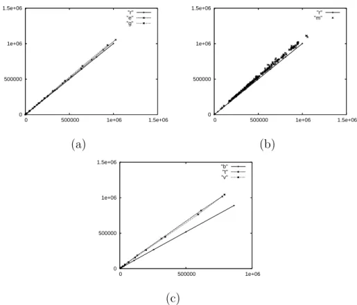
Let X be a set of points (i.e., a binary image) and n = #X be the number of points in X. We write m =Px∈X#ΠX(x). The number m corresponds to
the amount of memory which is necessary to store the projections of all the points of X. In Fig. 15, we plot the value of m with respect to n, for different families of binary images.
0 500000 1e+06 1.5e+06 0 500000 1e+06 1.5e+06 "r" "e" "g" 0 500000 1e+06 1.5e+06 0 500000 1e+06 1.5e+06 "r" "m" (a) (b) 0 500000 1e+06 1.5e+06 0 500000 1e+06 "b" "t" "v" (c)
Fig. 15. Plots of m (vertical axis) with respect to n (horizontal axis) for different 2D and 3D shapes. (a): families of 2D rectangles (r), ellipses (e) and zoomed gear images (g). (b): miscelanous 2D images (m), with rectangles (r) for comparison. (c): families of 3D boxes (b), torus (t) and zoomed vertebra images (v).
Annex B
The following figures show the distribution of the size of projections and ex-tended projections for a 2D and a 3D object.
0 0.1 0.2 0.3 0.4 0.5 0.6 0.7 0.8 0.9 1 0 1 2 3 4 0 0.1 0.2 0.3 0.4 0.5 0.6 0 1 2 3 4 5 6 (a) (b)
Fig. 16. (a): The distribution of #ΠX(x) for the 2D image of Fig. 7a. (b): The distribution of #Πe
X(x) for the 2D image of Fig. 7a.
0 0.1 0.2 0.3 0.4 0.5 0.6 0.7 0.8 0 1 2 3 4 5 6 7 8 9 10 0 0.05 0.1 0.15 0.2 0.25 0.3 0.35 0 1 2 3 4 5 6 7 8 9 10 11 12 13 14 15 16 (a) (b)
Fig. 17. (a): The distribution of #ΠX(x) for the 3D image of Fig. 9a. (b): The distribution of #ΠeX(x) for the 3D image of Fig. 9a.

![Fig. 9. (a): a view of a subset X of Z 3 (vertebra), generated thanks to a topolog- topolog-ically sound “Marching Cubes-like” algorithm [10]; (b,c,d): the bisector function, illustrated in an “X-ray” manner: the gray level of a point corresponds to the a](https://thumb-eu.123doks.com/thumbv2/123doknet/14121698.467760/15.892.155.690.104.606/vertebra-generated-marching-algorithm-bisector-function-illustrated-corresponds.webp)