Atmospheric histories and global emissions of the anthropogenic hydrofluorocarbons HFC-365mfc, HFC-245fa, HFC-227ea, and HFC-236fa

Atmospheric histories and global emissions

of the anthropogenic hydrofluorocarbons

HFC-365mfc, HFC-245fa, HFC-227ea, and HFC-236fa

The MIT Faculty has made this article openly available.

Please share

how this access benefits you. Your story matters.

Citation

Vollmer, Martin K. et al. “Atmospheric Histories and Global

Emissions of the Anthropogenic Hydrofluorocarbons HFC-365mfc,

HFC-245fa, HFC-227ea, and HFC-236fa.” Journal of Geophysical

Research 116.D8 (2011). ©2011 American Geophysical Union

As Published

http://dx.doi.org/10.1029/2010jd015309

Publisher

American Geophysical Union (AGU)

Version

Final published version

Citable link

http://hdl.handle.net/1721.1/74025

Terms of Use

Article is made available in accordance with the publisher's

policy and may be subject to US copyright law. Please refer to the

publisher's site for terms of use.

Atmospheric histories and global emissions of the anthropogenic

hydrofluorocarbons HFC

‐365mfc, HFC‐245fa, HFC‐227ea,

and HFC

‐236fa

Martin K. Vollmer,

Benjamin R. Miller,

Matthew Rigby,

Stefan Reimann,

Jens Mühle,

Paul B. Krummel,

Simon O

’Doherty,

Jooil Kim,

Tae Siek Rhee,

Ray F. Weiss,

Paul J. Fraser,

Peter G. Simmonds,

Peter K. Salameh,

Christina M. Harth,

Ray H. J. Wang,

L. Paul Steele,

Dickon Young,

Chris R. Lunder,

Ove Hermansen,

Diane Ivy,

Tim Arnold,

Norbert Schmidbauer,

Kyung‐Ryul Kim,

Brian R. Greally,

Matthias Hill,

Michael Leist,

Angelina Wenger,

and Ronald G. Prinn

Received 8 November 2010; revised 14 January 2011; accepted 31 January 2011; published 22 April 2011.

[1]

We report on ground

‐based atmospheric measurements and emission estimates of

the four anthropogenic hydrofluorocarbons (HFCs) HFC

‐365mfc (CH

CF

CH

CF

,

1,1,1,3,3

‐pentafluorobutane), HFC‐245fa (CHF

CH

CF

, 1,1,1,3,3

‐pentafluoropropane),

HFC

‐227ea (CF

CHFCF

, 1,1,1,2,3,3,3

‐heptafluoropropane), and HFC‐236fa

(CF

CH

CF

, 1,1,1,3,3,3

‐hexafluoropropane). In situ measurements are from the global

monitoring sites of the Advanced Global Atmospheric Gases Experiment (AGAGE), the

System for Observations of Halogenated Greenhouse Gases in Europe (SOGE), and

Gosan (South Korea). We include the first halocarbon flask sample measurements from the

Antarctic research stations King Sejong and Troll. We also present measurements of

archived air samples from both hemispheres back to the 1970s. We use a two

‐dimensional

atmospheric transport model to simulate global atmospheric abundances and to estimate

global emissions. HFC‐365mfc and HFC‐245fa first appeared in the atmosphere only

∼1 decade ago; they have grown rapidly to globally averaged dry air mole fractions of

0.53 ppt (in parts per trillion, 10

) and 1.1 ppt, respectively, by the end of 2010. In

contrast, HFC

‐227ea first appeared in the global atmosphere in the 1980s and has since

grown to

∼0.58 ppt. We report the first measurements of HFC‐236fa in the atmosphere.

This long

‐lived compound was present in the atmosphere at only 0.074 ppt in 2010. All

four substances exhibit yearly growth rates of >8% yr

at the end of 2010. We find rapidly

increasing emissions for the foam

‐blowing compounds HFC‐365mfc and HFC‐245fa

starting in

∼2002. After peaking in 2006 (HFC‐365mfc: 3.2 kt yr

, HFC

‐245fa: 6.5 kt yr

),

emissions began to decline. Our results for these two compounds suggest that recent

estimates from long

‐term projections (to the late 21st century) have strongly overestimated

emissions for the early years of the projections (

∼2005–2010). Global HFC‐227ea and

HFC

‐236fa emissions have grown to average values of 2.4 kt yr

and 0.18 kt yr

over

the 2008

–2010 period, respectively.

Citation: Vollmer, M. K., et al. (2011), Atmospheric histories and global emissions of the anthropogenic hydrofluorocarbons HFC‐365mfc, HFC‐245fa, HFC‐227ea, and HFC‐236fa, J. Geophys. Res., 116, D08304, doi:10.1029/2010JD015309.

1_{Laboratory for Air Pollution and Environmental Technology, Empa,} Swiss Federal Laboratories for Materials Science and Technology, Dubendorf, Switzerland.

2

Cooperative Institute for Research in Environmental Sciences, University of Colorado at Boulder, Boulder, Colorado, USA.

3

Center for Global Change Science, Massachusetts Institute of Technology, Cambridge, Massachusetts, USA.

4

Scripps Institution of Oceanography, University of California, San Diego, La Jolla, California, USA.

5

Centre for Australian Weather and Climate Research/CSIRO Marine and Atmospheric Research, Aspendale, Victoria, Australia.

6_{Atmospheric Chemistry Research Group, School of Chemistry,} University of Bristol, Bristol, UK.

7_{School of Earth and Environmental Sciences, Seoul National} University, Seoul, South Korea.

8_{Korea Polar Research Institute, Incheon, South Korea.} 9

School of Earth and Atmospheric Sciences, Georgia Institute of Technology, Atlanta, Georgia, USA.

10

Norwegian Institute for Air Research, Kjeller, Norway. 11

Research Institute of Oceanography, Seoul National University, Seoul, South Korea.

12

Deceased 7 December 2010. Copyright 2011 by the American Geophysical Union.

1.

Introduction

[2] Hydrofluorocarbons (HFCs) are anthropogenic

sub-stances predominantly used as refrigerants, foam blowing agents, fire retardants, and propellants. They replace the stratospheric ozone‐depleting chlorofluorocarbons (CFCs) and hydrochlorofluorocarbons (HCFCs), as these are being phased out under the regulations of the Montreal Protocol and its subsequent amendments and adjustments. HFCs have zero ozone depleting potential but many have a con-siderable Global Warming Potentials (GWPs). Hence they are included as one class of chemicals in the Kyoto Protocol of the United Nations Framework Convention on Climate Change (UNFCCC). Many countries, in particular those that have ratified the Kyoto Protocol, report their HFC emissions to the UNFCCC. The combined emissions reported to the UNFCCC cannot account for the total global emissions to the atmosphere, because of the large number of non-reporting countries. Furthermore, some of the HFCs are not required to be reported. For these reasons, emissions derived from atmospheric measurements (here termed ‘top‐down’ emissions) are a useful independent emission assessment tool. They also serve as an independent verifi-cation of the industry based production/consumption‐derived emissions [e.g., Velders et al., 2009; Intergovernmental Panel

on Climate Change, 2005], which we term ‘bottom‐up’

emissions. The purpose of this paper is to report on the atmospheric measurements of four HFCs (HFC‐365mfc, HFC‐245fa, HFC‐227ea, and HFC‐236fa), to character-ize their growth in the atmosphere, and to derive global emission estimates. Full‐scale commercial production of these four HFCs are believed to have started only recently. All four HFCs are relatively long‐lived in the atmosphere hence their atmospheric abundance is expected to grow. Their major sink is reaction with the hydroxyl radical (OH). Photolysis and reactions with Cl or O(1D) atoms are believed to be minor sinks (M. J. Kurylo, personal communication, 2010). The role of other sinks, for example, destruction through soil or aquatic environments, is largely unknown.

[3] HFC‐365mfc (CH3CF2CH2CF3, 1,1,1,3,3‐pentafluorobutane)

is mainly used for polyurethane structural foam blowing as a replacement for HCFC‐141b (CH3CCl2F), and to a minor

extent as a blend component for solvents [UNEP Technology and Economic Assessment Panel, 2010]. The first large‐ scale production of HFC‐365mfc started in the early 2000s in France, and it was predominantly used in Europe [Stemmler et al., 2007]. Using the first atmospheric obser-vations at Jungfraujoch (Switzerland) and Mace Head (Ireland) Stemmler et al. [2007] estimated European emis-sions of HFC‐365mfc at ∼1 kt yr−1for 2003 and 2004. Its atmospheric lifetime of 8.7 years is mainly a consequence of its removal through reaction with OH [Mellouki et al., 1995; Barry et al., 1997; S. P. Sander et al., Chemical kinetics and photochemical data for use in atmospheric studies, evalua-tion number 17 of the NASA panel for data evaluaevalua-tion, manuscript in preparation, 2011]; see Table 1. Its GWP on a 100 year time frame is estimated at 790–997 [Barry et al., 1997; Inoue et al., 2008]. HFC‐365mfc emissions are not required to be reported to the UNFCCC.

[4] HFC‐245fa (CHF2CH2CF3, 1,1,1,3,3‐pentafluoropropane)

is also used in polyurethane structural foam blowing, but is mainly marketed in North America [UNEP Technology and

Economic Assessment Panel, 2010]. Vollmer et al. [2006] published the first atmospheric measurements of this com-pound from both hemispheres and estimated its global emissions, which have more than doubled from∼2.3 kt yr−1 in 2003 to∼5.5 kt yr−1in 2005. The atmospheric lifetime of 7.7 years is similar to that of HFC‐365mfc, and HFC‐245fa is also largely removed by reaction with OH [Orkin et al., 1996; Nelson et al., 1995; Sander et al., manuscript in prep-aration, 2011]; see also Table 1. It has a GWP of 1030 on a 100 year time frame [Forster et al., 2007]. Like HFC‐365mfc, there is no obligation to report HFC‐245fa emissions to UNFCCC.

[5] HFC‐227ea(CF3CHFCF3, 1,1,1,2,3,3,3‐heptafluoropropane)

is mainly used as a fire retardant, replacing halon‐1301 (CF3Br), and as a propellant in metered‐dose inhalers (MDIs)

[UNEP Technology and Economic Assessment Panel, 2010]. Its atmospheric lifetime is estimated to be 38.9 years (Table 1) based on a considerable body of literature [Nelson et al., 1993; Zellner et al., 1994; Zhang et al., 1994; Tokuhashi et al., 2004; Hsu and DeMore, 1995; Wallington et al., 2004]. It has a GWP of 3220 on a 100 year time frame [Forster et al., 2007]. HFC‐227ea emissions are required to be reported to the UNFCCC by the contributing countries. Laube et al. [2010] have published the first atmospheric measurements and emission estimates of HFC‐227ea from samples collected at high altitude using aircrafts, and from firn air. Here we present the first long‐term ground‐based records of HFC‐227ea from in situ and air archive mea-surements in both hemispheres.

[6] HFC‐236fa (CF3CH2CF3, 1,1,1,3,3,3‐hexafluoropropane)

is used as a fire retardant [UNEP Technology and Economic Assessment Panel, 2010] and as a coolant in specialized applications [Intergovernmental Panel on Climate Change, 2005]. With an atmospheric lifetime of 242 years (Table 1 and Hsu and DeMore [1995], Gierczak et al. [1996], and Barry et al. [1997]) this compound is the second longest‐ lived HFC (after HFC‐23, CHF3[Naik et al., 2000]). With a

value of 9810, HFC‐236fa has the largest GWP on a 100 year time frame of all the four HFCs discussed here [Forster et al., 2007]. HFC‐236fa emissions are required to be reported to the UNFCCC by the contributing countries. To our knowl-edge, the data presented here are the first atmospheric mea-surements of this HFC.

2.

Materials and Methods

2.1. Stations and Data Records for in Situ Measurements

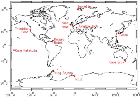
[7] The measurements of the four HFCs discussed here

stem from several fully intercalibrated affiliated measure-ment programs with differing data availability, summarized in Table 2 and shown in Figure 1. Specifically, data from in situ measurements are included from the following networks and institutions: the Advanced Global Atmospheric Gases Experiment (AGAGE) network operates instrumentation at the baseline stations at Mace Head (Ireland), Trinidad Head (California, USA), Ragged Point (Barbados), Cape Matatula (American Samoa), and Cape Grim (Tasmania, Australia); the SOGE network (System for Observations of Halogenated Greenhouse Gases in Europe), with instruments at Zeppelin (Spitsbergen), maintained by the Norwegian Institute for Air Research, NILU, and Jungfraujoch (Switzerland), maintained

by the Swiss Federal Laboratories for Materials Testing and Research, Empa; and an instrument at Gosan station on Jeju Island (South Korea) maintained by Seoul National Uni-versity (SNU). Previously published data, which we include in our analysis, are for selected periods for HFC‐365mfc from Mace Head (March 2003 to December 2004) and Jungfraujoch (December 2002 to December 2004 [Stemmler et al., 2007]) and of HFC‐245fa from Jungfraujoch (July 2004 to January 2006 [Vollmer et al., 2006]). Numerical values from the in situ measurements will soon be available from the Carbon Dioxide Information Analysis Center (CDIAC, http://cdiac.ornl.gov).

2.2. Flask Samples From Stations and Archived Air

[8] In addition to the in situ measurements from the

above‐mentioned stations, we also use measurements from samples collected at two stations in Antarctica, and archived air samples from both hemispheres.

[9] Beginning in 2007, air samples have been collected

from the South Korea Antarctic station King Sejong, King George Island (South Shetland Islands), maintained by the Korea Polar Research Institute (KOPRI). Weekly samples were filled with a metal‐bellows or Teflon‐coated neoprene membrane pump into 2.5 L internally electropolished stainless steel flasks. Samples were also collected from the Norwegian Antarctic station Troll, maintained by NILU. These samples were collected in 2 L internally electro-polished stainless steel flasks using a metal‐bellows pump. The Antarctic air samples were analyzed on Medusa in-struments (see section 2.3) at Jungfraujoch or Empa. The mean measurement precisions (1s standard deviations from repeat measurements of individual flasks) for these Antarctic samples are 2.3% for HFC‐365mfc, 1.9% for HFC‐245fa, 2.0% for HFC‐227ea, and 6.1% for HFC‐236fa. Numerical values and more detailed information are provided in the auxiliary material.1

[10] Our analysis includes measurements of the Cape

Grim Air Archive (CGAA) for the Southern Hemisphere (SH), collected since 1978 at the Cape Grim Baseline Air Pollution Station for archival purposes [Langenfelds et al., 1996; Krummel et al., 2007]. For most of the∼60 samples, air was collected into 35 L internally electropolished stain-less steel canisters using cryogenic techniques. However some samples were collected under slightly different

con-ditions [Langenfelds et al., 1996]. For many of the older samples, one or more of the four HFCs were absent in the chromatograms. Very small chromatographic peaks required careful and consistent integration to avoid nonlinear inte-gration effects. Numerical values and more details on the CGAA measurements are given in the auxiliary material.

[11] We also include measurements from ∼100 archived

air samples of the Northern Hemisphere (NH). These sam-ples cover the period from 1973 to present and were col-lected at multiple stations in the USA. The majority of the samples were provided by the Scripps Institution of Oceanography (SIO); see auxiliary material for details. These samples were filled during periods when the sites were expected to intercept background air, but with varying filling techniques and for purposes other than the recon-struction of atmospheric trace gas histories. For these rea-sons, the data set contained outliers. Higher mole fractions than expected were caused by contamination or sampling of pollution, and reduced mole fractions were mainly caused by retention of the compounds on drying agents during the filling process. Samples were rejected through an iterative process based on their deviation from a fit through all data. This process is supported by similar selection results for various compounds [e.g., Mühle et al., 2010; Rigby et al., 2010]. The final archived NH data set (∼60 samples) showed good agreement with in situ measurements, when available. The numerical results and more details are given in the auxiliary material.

2.3. Measurement Techniques

[12] Two similar measurement technologies were

em-ployed, both based on gas chromatography–mass spectrometry (GC‐MS) and cryogenic sample preconcentration techniques. An earlier instrument, termed ADS (Adsorption‐Desorption‐ System [Simmonds et al., 1995]), was used for several years at the Zeppelin, Mace Head, Jungfraujoch, and Cape Grim stations. These instruments were replaced by a GC‐MS technique referred to as‘Medusa’ [Miller et al., 2008], which has enhanced sampling frequency, compound selection, and measurement precisions (Zeppelin was converted only in September 2010). The Medusa is also used at all other stations with in situ measurements listed in Table 2.

[13] For the Medusa measurements, 2 L of sample are

preconcentrated on one trap and subsequently cryofocused on a second trap, both held at∼−160°C [Miller et al., 2008]. The analytes are then passed through a single main capillary chromatography column (CP‐PoraBOND Q, 0.32 mm ID ×

25 m, 5 mm, Varian Chrompack) with temperature and

Table 1. Atmospheric Lifetimes, Global Warming Potentials (GWP) on a 100 Year Time Basis, and OH Reaction Rates of HFC‐365mfc, HFC‐245fa, HFC‐227ea, and HFC‐236fa

Lifetimea_(years)

GWPsb Reaction With OHc(k in cm3molecule−1s−1and T in K) Total OH (Tropospheric) Stratospheric

HFC‐365mfc 8.7 9.3 125 794–997d (1.8 ± 1.3) × 10−12exp(−(1660 ± 100)/T) HFC‐245fa 7.7 8.2 116 1030 (0.61 ± 0.12) × 10−12exp(−(1330 ± 150)/T) HFC‐227ea 38.9 44.5 310 3220 (0.63 ± 0.115) × 10−12exp(−(1800 ± 150)/T) HFC‐236fa 242 253 5676 9810 (1.45 ± 1.15) × 10−12exp(−(2500 ± 150)/T)

a_{Montzka and Reimann [2011].} b

Forster et al. [2007] unless stated otherwise. c_{Sander et al. (manuscript in preparation, 2011).} d

Inoue et al. [2008].

1

Auxiliary material data sets are available at ftp://ftp.agu.org/apend/jd/ 2010jd015309.

pressure ramping using Agilent Technologies series 6890 GCs. The compounds are detected with a quadrupole MS (Agilent Technologies series 5973 and 5975) in selec-tive ion mode. Some of the Medusa instruments differ slightly from the design described by Miller et al. [2008], these do not however alter the measurement principle or negatively influence the analysis. Identification of the sub-stances was conducted on the Jungfraujoch Medusa and on a GC‐MS‐ADS at the Empa lab using synthetic air samples spiked with aliquots of the pure substances, and with the commercial standards and the tanks used for the primary scale definitions. The elution sequence for the four HFCs, as compared to other routinely measured compounds, showed some variations for individual instruments; but in general,

HFC‐227 elutes on the tail of CFC‐12 (CCl2F2), HFC‐236fa

elutes shortly before HCFC‐142b (CH3CClF2) and HFC‐

245fa shortly thereafter, and HFC‐365mfc elutes in the proximity of CFC‐11 (CCl3F). The following mass over

charge ratios (m/z) were used for identification and the first of each pair was used for quantification: 151 and 82 for HFC‐227ea, 133 and 69 for HFC‐236fa, 115 and 51 (some stations 115 and 69) for HFC‐245fa [Vollmer et al., 2006] and 133 and 65 for HFC‐365mfc [Stemmler et al., 2007]. Because of their low abundances in the samples, peak sizes were initially comparably small but grew as the mole frac-tions increased in the samples. This is reflected in the mea-surement precisions. They are given here as ranges derived from the first years of measurements for each compound to

Figure 1. Sampling locations.

Table 2. Station List and Data Availability of HFC‐365mfc, HFC‐245fa, HFC‐227ea, and HFC‐236faa

Station Network/ Institution Latitude (°N) Longitude (°E) Instrument

Data Availability (mm/yyyy)

HFC‐365mfc HFC‐245fa HFC‐227ea HFC‐236fa Zeppelin SOGE 78.9 11.9 ADS 12/2006 to 12/2010 – – – Mace Head AGAGE 53.3 −9.9 ADS 03/2003 to 03/2005 – – – Mace Head AGAGE 53.3 −9.9 Medusa 07/2005 to 12/2010 11/2006 to 12/2010 10/2006 to 12/2010 10/2006 to 12/2010 Jungfraujoch SOGE 46.5 8.0 ADS 12/2002 to 03/2008 07/2004 to 03/2008 10/2004 to 03/2008 – Jungfraujoch SOGE 46.5 8.0 Medusa 04/2008 to 12/2010 04/2008 to 12/2010 04/2008 to 12/2010 04/2008 to 12/2010 Trinidad Head AGAGE 41.0 −124.1 Medusa 05/2005 to 12/2010 12/2007 to 12/2010 10/2007 to 12/2010 10/2007 to 12/2010 NH sites SIO and other – – Medusa flasks 10/1973 to 12/2010 10/1973 to 12/2010 10/1973 to 12/2010 10/1973 to 12/2010 Gosan SNU 33.3 126.2 Medusa 11/2007 to 12/2010 02/2008 to 12/2010 11/2007 to 12/2010 05/2008 to 12/2010 Ragged Point AGAGE 13.2 −59.4 Medusa 05/2006 to 12/2010 12/2007 to 12/2010 11/2007 to 12/2010 10/2007 to 12/2010 Cape Matatula AGAGE −14.2 −170.6 Medusa 05/2006 to 12/2010 11/2007 to 12/2010 10/2007 to 12/2010 10/2007 to 12/2010 Cape Grim AGAGE −40.7 144.7 ADS 03/2004 to 02/2005 – – – Cape Grim AGAGE −40.7 144.7 Medusa 05/2005 to 12/2010 06/2006 to 12/2010 06/2006 to 12/2010 09/2006 to 12/2010 Cape Grim CSIRO/BoM −40.7 144.7 Medusa flasks 04/1978 to 12/2010 04/1978 to 12/2010 04/1978 to 12/2010 04/1978 to 12/2010 King Sejong KOPRI −62.2 −58.8 Medusa flasks 02/2007 to 12/2009 02/2007 to 12/2009 02/2007 to 12/2009 02/2007 to 12/2009 Troll NILU −72.0 2.5 Medusa flasks 03/2008 to 12/2009 03/2008 to 12/2009 03/2008 to 12/2009 03/2008 to 12/2009

a

Stations are listed in latitudinal order from north to south. Data availability for in situ and flask records with start and end dates (12/2010 indicates ongoing measurements). SOGE, System for Observations of Halogenated Greenhouse Gases in Europe; AGAGE, Advanced Global Atmospheric Gases Experiment; SIO, Scripps Institution of Oceanography; SNU, Seoul National University; CSIRO/BoM, CSIRO Marine and Atmospheric Research/Australian Bureau of Meteorology; KOPRI, Korea Polar Research Institute; NILU, Norwegian Institute for Air Research. See text for the details on the instrument types ADS (Adsorption Desorption System) and Medusa.

their typical precisions (1 s) at the end of the records used here. These precisions are estimated from the repeated working (quaternary) standard measurements (excluding those spiked with these HFCs). They are estimated for HFC‐ 365mfc at 15–5%, for HFC‐245fa at 9–3%, for HFC‐227ea at 6–3%, and for HFC‐236fa at 12–10%.

2.4. Instrument Calibrations

[14] For the continuous Medusa measurements, ambient

air samples are analyzed every 2 h (every 4 h for GC‐MS‐ ADS) and bracketed by measurements of quaternary stan-dards to detect and correct for short‐term instrumental drift. The quaternary standards are ∼60 bar whole‐air in 35 L internally electropolished stainless steel canisters (Essex Cryogenics). They are filled with modified oil‐free diving compressors (RIX Industries, California), with the exception of Cape Grim, where they are typically filled cryogenically. To allow a more precise correction of instrumental drift some quaternary standards at Cape Grim and Jungfraujoch were spiked to about double (HFC‐245fa and HFC‐227ea), and 10 times (HFC‐236fa) ambient air signals. Quaternary standards are directly compared to higher‐ranking traveling standards (tertiary standards), which are exchanged between SIO and the individual sites. These tertiary standards are filled during relatively clean‐air conditions at Trinidad Head using modified diving compressors (SA‐3 and SA‐6, RIX Industries), and measured at SIO against secondary stan-dards before and after usage at the sites. For the AGAGE sites and Gosan, quaternary‐tertiary comparisons are con-ducted weekly to detect potential mole fraction drift of the measured compounds in these canisters. For the four HFCs under discussion, there was no indication of drift during storage, allowing us to conclude that these four HFCs are stable in our sample canisters.

2.5. Calibration Scales, Their Propagations, and Uncertainties of the Reported Data

[15] The primary calibration scales for the four HFCs

discussed here were produced at Empa and are maintained at SIO. They are linked into the SIO calibration system via transfer of several sample canisters between the two in-stitutions. All other stations and institutions are tied to these HFCs scales through the distribution of tertiary standards. All measurement results and the corresponding data pre-sented here are reported on the calibration scales outlined next.

[16] The HFC‐365mfc measurements are reported on the

Empa‐2003 calibration scale [Stemmler et al., 2007]. This scale is based on repeated preparations of gravimetrically diluted aqueous solutions. Based on the technical descrip-tion by Stemmler et al. [2007] of this process, we estimate an accuracy of 10% for this scale.

[17] For HFC‐245fa [Vollmer et al., 2006] and HFC‐227ea

a combined primary standard (termed 227gld) was produced by dynamic dilution of a commercial high‐concentration (24.9 ppb) standard (Apel‐Riemer) with purified synthetic air. This procedure is described by Vollmer et al. [2006] and has led to the Empa‐2005 calibration scales for HFC‐245fa and HFC‐227ea with estimated accuracies of 6%.

[18] The primary scale for HFC‐236fa was produced by the

dilution of an aliquot of a commercial high‐concentration (20 ppb) standard (Apel‐Riemer) with purified synthetic air,

producing a primary standard termed PP‐001. As was the case for 227gld, several reference compounds (here HFC‐ 134a, carbonyl sulfide, HFC‐245fa, HFC‐227ea) were added to the original mixture by the manufacturer. The ref-erence compounds in PP‐001 were then measured against standards of known compositions. Using results from these reference gases and accurate pressure measurements, a con-centration was assigned for HFC‐236fa in PP‐001 with an estimated accuracy of 6%. This dilution defines the Empa‐ 2009 calibration scale for HFC‐236fa.

[19] In addition to the first type of uncertainty (the above

scale‐defining uncertainty) we attribute another two types of uncertainties to the final measurement results. The second type derives from the propagation of the scale through a series of transfer standards (propagation uncertainty). For this we assume on average three subsequent transfer stan-dards between primary and quaternary stanstan-dards. The third type consists of the measurement precision as estimated by the repeated quaternary standard measurements (sample uncertainty). In relative mole fraction terms, the propagation and sampling uncertainties decreased strongly over time because of improved measurements (larger chromatographic peaks) as the mole fractions in transfer standards and air samples/quaternary standards increased rapidly over time. Uncertainties based on systematic analytical errors (e.g., trapped air volume) are comparably insignificant, and hence we ignore them here. For the time periods covering the first in situ measurements to the end of the presented record, the overall accuracies of the measurement results based on the 3 types of uncertainties are estimated as follows and the improvement can be assumed to be roughly linear over the time span of our data records: HFC‐365mfc: 32–14%; HFC‐

245fa: 19–8%; HFC‐227ea: 13–8%; HFC‐236fa: 25–21%.

2.6. Bottom‐Up Emission Estimates

[20] One of the goals of this paper is to estimate global

emissions of these four HFCs. Here we first introduce the available bottom‐up emissions, which will serve as a basis for comparisons to our own modeled emissions in section 3.3. We primarily use the emission estimates by Ashford et al. [2004a, 2004b] and the ‘UNFCCC emissions’ (data in the UNFCCC Common Reporting Format (CRF), which are available at http://unfccc.int/di/DetailedByParty.do).

[21] Ashford et al. [2004b] provide global emission

esti-mates for HFC‐365mfc, HFC‐245fa, and HFC‐227ea based on information from the industry, and from market surveys [Ashford et al., 2004a]. For their estimates, they use param-etrized emission functions, which take into account the delays in the emissions due to slow release of these substances from‘banks.’ While giving detailed quantitative information on the lifecycles for other foam‐blowing substances, Ashford et al. [2004b] list the total emissions only for HFC‐365mfc and HFC‐245fa.

[22] For HFC‐227ea, Ashford et al. [2004b] distinguish

between usage as a fire retardant, an MDI propellant, and to a lesser extent, as a foam‐blowing agent. For the first two uses, they provide linear emission functions. According to their estimates, emissions from MDI start in 1992, emissions from fire extinguishers in 1997, followed by emissions from foams considerably later. The fire extinguisher emissions are the predominant source, for example, in 2010 they were

0.54 kt, compared to 0.15 kt from MDI and 0.10 kt from foam blowing.

[23] The UNFCCC emissions estimates are derived from

the CRF tables provided by individual countries on an annual basis starting in 1990. We use the 2009 CRF updated data (as countries can retrospectively adjust earlier years). In general, the reporting countries provide emissions for indi-vidual HFCs. Some countries pool HFC emissions for pro-ducer confidentiality reasons. HFC‐365mfc is not listed as an individual compound in the UNFCCC CRF, and hence there are no emissions reported from any country. HFC‐ 245fa is not listed either, but instead its isomer HFC‐245ca is listed, presumably because originally this compound was believed to be more widely used than HFC‐245fa. Conse-quently, no country has reported HFC‐245fa emissions except for the USA, which include HFC‐245fa in a pooled emission report on a few HFCs. For a few European countries with pooled emission estimates, we estimate the HFC‐227ea and HFC‐236fa fractions, using the same fractions as reported for the remaining countries of the European Community. For the USA, we are unable to provide a rea-sonable extraction of HFC‐227ea and HFC‐245fa from their pooled emissions, and subsequently exclude any potential emissions of these two compounds from this country. In summary, because of this exclusion and of many countries not reporting to the UNFCCC, the UNFCCC estimates are most likely a large underestimate of the total global emissions.

[24] In addition to the Ashford et al. [2004b] and UNFCCC

estimates, emissions are also estimated by the EDGAR project (Emission Database for Global Atmospheric Research (EDGAR): European Commission, Joint Research Centre

(JRC)/Netherlands Environmental Assessment Agency

(PBL), http://edgar.jrc.ec.europa.eu) [Olivier et al., 2002]. However for HFC‐365mfc, HFC‐245fa, and HFC‐227ea, the values in the EDGAR global data sets for the release version 4.0 are entirely based on the results by Ashford et al. [2004b], and those for HFC‐236fa on the UNFCCC (CRF 2008) reports (J. Olivier, personal communication, 2010). Therefore the EDGAR emissions do not provide any addi-tional information for our study and are mentioned here only for completeness.

[25] We find four additional global emissions data sets in

the literature, which provide long‐term emission projections under various scenarios. Although the focus of these pro-jections is on the middle and end of the 21st century, it is nevertheless instructive to assess the differences between our estimates and the early years of these projections. The first data set is part of the International Panel on Climate Change (IPCC) Special Report on Emission Scenarios, often abbreviated SRES [Nakicenovic et al., 2000; Fenhann, 2000] (and supplemented 2010 data from http://sres.ciesin.org). This IPCC report includes HFC‐365mfc and HFC‐245fa and treats the two substances combined, justified by their similar climate effects. These SRES emissions are listed under four different scenarios (A1, A2, B1, B2) for 1990– 2100. The second data set is by Intergovernmental Panel on Climate Change [2005] and provides projected emissions for all four HFCs for 2015 under a business‐as‐usual and a mitigation scenario. The third data set contains more recent emission projections by Velders et al. [2009] also for the combined emissions of HFC‐245fa and HFC‐365mfc.

These projections are given for two scenarios spanning 1990–2050. The fourth long‐term emission projections are those used for the upcoming IPCC Assessment Report AR5 [Moss et al., 2010]. The various scenarios are termed ‘Representative Concentration Pathways’ (RCP) with data available from http://www.iiasa.ac.at. Of the four scenarios, which range over 2000–2100, three RCPs have emission estimates for HFC‐245fa and HFC‐227ea but do not include the other two HFCs.

2.7. Global Chemical Transport Model and Inverse

Method

[26] The AGAGE two‐dimensional (2D), 12‐box

atmo-spheric transport model [Cunnold et al., 1983, 1994, 1997] was used to simulate semihemispheric mole fractions that could be compared to the observations. The model was also used to estimate the sensitivity of the mole fractions to changes in annual semihemispheric emissions. The atmo-spheric boxes cover 4 semihemispheres from 0°–30° (termed ‘tropics’) and 30°–90° (termed ‘extratropics’) in each hemi-sphere. There are three vertical layers, which represent the lower troposphere, the upper troposphere, and the strato-sphere with divisions at 500 hPa and 200 hPa. The latitudinal separations were chosen such that boxes in each vertical band contain equal air masses. The model transport para-meters are based on climatology, and have been optimally tuned so that CFC measurements were well reproduced at AGAGE sites [Cunnold et al., 1997]. The model transport parameters and OH concentrations are seasonally varying and interannually repeating, and the average OH concen-tration has been optimally determined using methyl chlo-roform measurements [Prinn et al., 2005].

[27] The sensitivity of monthly background mole fractions

at each observation site to annual pulses of emissions from each hemisphere was calculated and used to determine hemispheric release rates. A Bayesian inverse method was used, which determines emissions using the measurements and model‐calculated sensitivities in addition to independent prior information [e.g., Enting et al., 1995; Tarantola, 2005]. Prior emissions information was obtained from the invento-ries outlined in section 2.6, with Ashford et al. [2004b]

emissions being used for HFC‐365mfc and HFC‐245fa,

UNFCCC emissions for HFC‐236fa and an average of the two for HFC‐227ea. Whilst uncertainty estimates are not available from these inventories, initial predictions of the atmospheric mole fractions using the bottom‐up estimates revealed significant discrepancies from the measurements, on the order of 100% for some compounds. Therefore, we assumed a 100% uncertainty on the prior emissions, with a minimum uncertainty equal to the inventory mean, taken from the year of onset of emissions (to avoid the prior uncertainty going to zero). UNFCCC emissions were not available for 2008–2010, so we linearly extrapolated the 2006–2007 emissions throughout this period.

[28] An initial estimate of the latitudinal emissions

dis-tribution was based on the HCFC‐22 emissions derived by Miller et al. [1998]. However, as outlined above, emissions of HFC‐365mfc were expected to originate entirely from Europe. Therefore, emissions for this compound were ini-tially assumed to originate entirely from the NH‐extratropical box in the model. Whilst the interhemispheric emissions distribution was adjusted in the inversion, it was found that

hemispheric emissions were not well resolved by the mea-surements. Therefore, only the better‐resolved global avera-ges are shown below. However, it is noteworthy that for HFC‐365mfc, the inversion resulted in more than 99% of the emissions originating from the NH extratropical box. For each compound, the initial modeled atmospheric mole fractions in 1978 were assumed to be zero.

[29] The uncertainty of each observation used in the

inversion included the measurement precisions defined above, and an estimate of the effect of variations in sampling frequency, and of model‐data mismatch [Chen and Prinn, 2006]. The total uncertainty was calculated as the squared sum of these terms. Sampling frequency uncertainty was estimated as the monthly baseline variability, divided by the square root of the number of measurements. Model‐data mismatch was taken to be the measured monthly baseline variability, and was therefore a measure of the inability of the model to resolve submonthly mole fractions. The baseline variability was not available for measurements of archived samples or at flask measurement sites. Therefore, we estimated the variability for these data points using the mean variability at the closest high‐frequency monitoring site, scaled by the mean mole fraction.

[30] The uncertainties calculated in the inversion optimally

combine the prior and measurement uncertainties [e.g., Tarantola, 2005]. The presented uncertainties also include box model parametric uncertainties (which includes the uncertainty associated with the use of interannually repeat-ing transport), estimated by runnrepeat-ing the inversion 100 times with perturbed model parameters. Also included were per-turbations of the HFC‐OH reaction rate and OH concentra-tion, the magnitude of which were given by the uncertainties from Sander et al. (manuscript in preparation, 2011) and Prinn et al. [2005], respectively. Finally, the uncertainty associated with the HFC calibration scale was included in the final estimates.

3.

Results and Discussion

3.1. Atmospheric Abundances and Growths

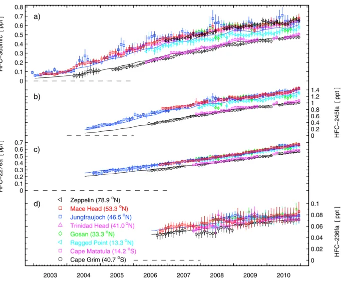
[31] The atmospheric records from eight measurement sites

are shown in Figure 2. There we show monthly means of background‐filtered data following a statistical filter algorithm [O’Doherty et al., 2001; Cunnold et al., 2002]. The longest in situ records are generally those from Jungfraujoch and Mace Head in the NH and from Cape Grim in the SH. Mole fractions (in dry air) for all four compounds are very small and in the ppt (parts per trillion, 10−12) and sub‐ppt range.

[32] The record for HFC‐365mfc is the longest of all four

HFCs (Figure 2a). At Jungfraujoch and Mace Head the mole fractions were below 0.1 ppt in 2003 [Stemmler et al., 2007] and have reached 0.65 ppt by the end of 2010 at these and other extratropical NH sites. Our model results show a global mean mole fraction of 0.53 ppt in 2010 and a steadily increasing growth rate peaking at∼0.09 ppt yr−1in 2005 and 2006 (Table 3). The growth has since declined to∼0.05 ppt yr−1 (10% yr−1) in 2010. The Jungfraujoch record shows some periods of elevated mole fractions compared to other NH sites. This is partially caused by a higher continental ‘background’ [O’Doherty et al., 2009; Reimann et al., 2004] and by some limitations of the filtering algorithm to separate background from pollution data at this site, which

experi-ences frequent HFC‐365mfc pollution episodes. A similar computational difficulty to define ‘background’ is seen at Gosan because the measured air originates from a large latitudinal band that is characterized by a latitudinal gradient in‘background’ air. Longer periods of southerly advection lead to reduced monthly mixing ratios at this site for all four compounds (Figure 2). HFC‐365mfc is the only one of the four HFCs currently measured at the high‐latitude site Zeppelin.

[33] The reduced mole fractions in the SH, as compared to

the NH, is a well‐known feature of anthropogenic trace gases with predominantly NH emissions. However, for HFC‐365mfc the gradient between the more northerly NH stations and those in the SH is larger than for other com-pounds. In addition, our record at Ragged Point shows mole fractions for HFC‐365mfc that are significantly closer to those of the SH, as compared to the other three HFCs and other substances measured at these stations (e.g., SF6[Rigby

et al., 2010]). While the magnitude of the latitudinal gra-dients is generally also driven by the atmospheric growth rates of these anthropogenic substances, this cannot be the cause for this feature observed for HFC‐365mfc, as the relative growth rates of all four HFCs are similar and could therefore not explain the unusual Ragged Point record. This difference is likely a cause of HFC‐365mfc’s unique lati-tudinal emission pattern. HFC‐365mfc is predominantly released in Europe [Stemmler et al., 2007; Vollmer et al., 2006] and has negligible emissions from the USA and East Asia, both being regions that span latitude bands farther south than Europe.

[34] HFC‐245fa, which has a shorter record, grew from

∼0.2 ppt in 2004 at Jungfraujoch to 1.4 ppt by the end of 2010 (Figure 2b). HFC‐245fa’s modeled global mean mole fraction in 2010 was 1.1 ppt (Table 3). The modeled growth rate peaked at 0.24 ppt yr−1in 2006 and has since declined to 0.15 ppt yr−1(13% yr−1) in 2010. With this large growth rate, HFC‐245fa is the only one of the four HFCs presented that has reached NH mole fractions >1 ppt.

[35] Upon visual inspection, HFC‐227ea is the compound

with the most linear growth since measurements started in 2004 at Jungfraujoch (Figure 2c). The mole fractions have increased since then and have now reached a global mean value of 0.58 ppt (Table 4). HFC‐227ea’s modeled global growth rate has also increased and is highest at the end of the record at 0.07 ppt yr−1, corresponding to a relative growth of 12% yr−1. The interhemispheric offset for HFC‐ 227ea appears remarkably constant and the lag time of the SH to the NH is only∼1 year, whereas for HFC‐365mfc and HFC‐245fa the lag is >3 years. Given similar relative growth rates and long lifetimes, this is to first approximation suggestive of a more balanced emission pattern between the two hemispheres for HFC‐227ea compared to HFC‐365mfc and HFC‐245fa. The fact that the Ragged Point record is not offset from the other NH sites supports this hypothesis.

[36] The mole fractions of HFC‐236fa are approximately

1 order of magnitude lower than those of the other three HFCs or any other of the compounds measured within the AGAGE and SOGE networks (Figure 2d). They were ∼0.05 ppt at the beginning of the in situ record in 2006 (Mace Head and Cape Grim). Our modeled global mean mole fraction for 2010 is 0.074 ppt with maximum growth rates occurring in 2008 (0.008 ppt yr−1or 10% yr−1). Large

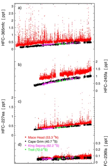
uncertainties in the quantification of the small GC‐MS peaks cause large uncertainties in the calibration‐scale propagation. This is the cause for the discontinuity observed in the first 2 years of the in situ record at Cape Grim. Also, there is an apparent mismatch between our modeled SH extratropical abundances and the CGAA observations for 1993–2003 (Figure 4); However the observations are within the relatively large uncertainties of the modeled record for that period (not shown in Figure 4; see auxiliary material). [37] The atmospheric records from the Antarctic stations

King Sejong and Troll are shown in Figure 3 along with the in situ records from Cape Grim and Mace Head; none are filtered for pollution events. For each of the substances, the mole fractions at King Sejong, Troll and Cape Grim agree within the combined uncertainties despite the 31° latitude difference. This agreement for these long‐lived compounds is an illustration of the well‐mixed lower atmosphere in this part of the world.

[38] For Mace Head and Cape Grim in Figure 3 we have

chosen to show the full in situ records without background

filtering to illustrate the variable magnitudes of pollution episodes at various sites. For example, Cape Grim is rarely reached by air masses with significant HFC pollution, while Mace Head is influenced by occasional large pollution events from the European continent, particularly for HFC‐ 365mfc. While the general differences between the various sites is expected and known from earlier work using mea-surements of trace gases at these stations [e.g., Prinn et al., 2000], we find large differences, for most sites, in the pol-lution pattern of one compound versus the other at all stations. Prominent examples are HFC‐365mfc and HFC‐245fa. We find larger and more frequent HFC‐365mfc pollution events as compared to HFC‐245fa for the European stations Mace Head and Jungfraujoch, and for Aspendale (Victoria, Aus-tralia, semiurban measurements, not included in the global analysis, data provided by CSIRO). In contrast results from the USA station Trinidad Head and from La Jolla (San Diego, California, semiurban measurements not included in the global analysis, data provided by SIO) show HFC‐245fa pollution episodes dominating over those for HFC‐365mfc. Figure 2. Atmospheric records of the hydrofluorocarbons (HFCs) (a) HFC‐365mfc, (b) HFC‐245fa,

(c) HFC‐227ea, and (d) HFC‐236fa from in situ measurements. The monthly mean mixing ratios shown are based on background selected data. The vertical bars denote the 1s standard deviation of the monthly means. The solid blue and black lines are the mean Northern and Southern Hemisphere model results, respectively. The horizontal dashed lines are supporting visual guides of the zero mole fractions.

This is likely a consequence of the ban on HFC‐365mfc use in foam applications by the USA Environmental Protection Agency (EPA) until September 2009 (http://edocket.access. gpo.gov/2009/E9‐23470.htm). This example demonstrates how regional usage and regulations in the HFC foam blowing sector influence the atmospheric records, which was much less prominent during the era when use of the CFCs and HCFCs was dominant.

[39] Another example of the influence of regional

emis-sion patterns on atmospheric measurements is HFC‐227ea. Even though its global emissions are similar in magnitude

to those of HFC‐365mfc, Mace Head and Jungfraujoch

show comparably fewer and less intense pollution events. This is presumably due to usage restrictions in some Euro-pean countries (e.g., banned in fire retardant applications in Switzerland). For HFC‐236fa, except for Gosan, none of the AGAGE or SOGE stations show significant pollution events. While this is also true for the urban measurements at Aspendale, those at La Jolla show large and frequent HFC‐ 236fa pollution events; however more quantitative inspec-tion of these features is beyond the scope of this paper.

3.2. Air Archive Results

[40] The results from the archived air measurements are

shown in Figure 4. HFC‐365mfc and HFC‐245fa are not

detectable in the archived air samples until about 2003. These findings are in line with those of Stemmler et al. [2007] and Vollmer et al. [2006] and suggest that these substances are only recent creations of industry. These are by far the youngest of all halogenated compounds reported on in the atmospheric science literature. However, within about 5 years, HFC‐365mfc grew by ∼0.5 ppt and HFC‐ 245fa by ∼1.0 ppt in the NH. We relate this late market introduction to the interim uses of HCFCs (particularly HCFC‐141b) as a consequence of the CFC phase out. While HCFCs are now banned from use in new products in non‐ Article 5 (developed) countries within the Montreal Protocol, Article‐5 (developing) countries will be subject to a phase‐ out beginning with a freeze in 2013. With this upcoming phase‐out, further large increases of atmospheric HFC‐ 365mfc and HFC‐245fa can be expected if these two sub-stances will be the replacement compounds of choice. In addition, banks of these compounds in structural foams are increasing at rapid rates and will potentially comprise a growing fraction of their emissions.

[41] HFC‐227ea shows a very different atmospheric

his-tory. This compound appears in the mid‐1980s and has grown steadily since the mid‐1990s, although at lower rates than HFC‐365mfc and HFC‐245fa. We speculate that the relatively early onset is due to its early use as a fire retar-Table 3. Mean Global Mole Fractions, Their Uncertainties (MF‐U), Annual Growth Rates, Emissions, and Their Uncertainties (E‐U) for the Hydrofluorocarbons HFC‐365mfc and HFC‐245fa From the 12‐Box Model Calculationsa

Year HFC‐365mfc HFC‐245fa Mole Fraction (ppt) MF‐U 1 s (ppt) Growth (ppt yr−1) Emissions (kt yr−1) E‐U 1 s (kt yr−1) Mole Fraction (ppt) MF‐U 1 s (ppt) Growth (ppt yr−1) Emissions (kt yr−1) E‐U 1 s (kt yr−1) 1978 0.002 0.031 −0.001 −0.03 ±0.79 0.000 0.035 −0.001 −0.03 ±1.07 1979 0.001 0.032 −0.001 −0.02 ±0.82 0.000 0.048 −0.002 −0.05 ±1.58 1980 0.000 0.040 −0.001 −0.03 ±0.85 0.002 0.082 0.009 0.18 ±1.81 1981 0.000 0.047 −0.001 −0.03 ±0.78 0.000 0.110 −0.014 −0.27 ±1.34 1982 0.000 0.054 0.003 0.06 ±0.84 0.000 0.118 0.013 0.24 ±1.74 1983 0.003 0.061 0.003 0.07 ±0.85 0.002 0.124 −0.007 −0.11 ±1.69 1984 0.005 0.065 0.002 0.08 ±0.85 0.000 0.119 −0.003 −0.06 ±1.76 1985 0.004 0.064 −0.006 −0.11 ±0.83 0.000 0.119 0.004 0.07 ±1.79 1986 0.001 0.060 0.000 −0.00 ±0.79 0.000 0.122 −0.001 −0.01 ±1.33 1987 0.003 0.062 0.003 0.08 ±0.82 0.000 0.116 0.000 0.00 ±1.50 1988 0.003 0.066 −0.002 −0.03 ±0.80 0.001 0.114 0.001 0.02 ±1.56 1989 0.003 0.067 0.001 0.01 ±0.83 0.000 0.115 −0.003 −0.06 ±1.58 1990 0.005 0.067 0.005 0.12 ±0.77 0.000 0.121 0.004 0.07 ±1.30 1991 0.008 0.068 −0.000 0.03 ±0.83 0.001 0.114 −0.002 −0.03 ±1.61 1992 0.005 0.068 −0.006 −0.11 ±0.83 0.003 0.107 0.005 0.12 ±1.59 1993 0.001 0.066 −0.001 −0.04 ±0.81 0.000 0.109 −0.012 −0.22 ±1.55 1994 0.002 0.067 0.003 0.07 ±0.79 0.000 0.114 0.008 0.12 ±1.41 1995 0.004 0.066 0.001 0.05 ±0.75 0.000 0.117 −0.002 −0.03 ±1.31 1996 0.002 0.064 −0.005 −0.10 ±0.76 0.004 0.115 0.008 0.16 ±1.35 1997 0.004 0.063 0.008 0.18 ±0.68 0.003 0.113 −0.007 −0.11 ±0.98 1998 0.010 0.061 0.003 0.12 ±0.73 0.000 0.103 −0.005 −0.13 ±1.13 1999 0.011 0.060 −0.002 0.01 ±0.75 0.000 0.100 0.009 0.17 ±1.27 2000 0.013 0.059 0.007 0.18 ±0.81 0.000 0.111 −0.009 −0.17 ±1.50 2001 0.019 0.059 0.005 0.18 ±0.80 0.000 0.120 0.000 −0.03 ±1.49 2002 0.030 0.058 0.017 0.46 ±0.79 0.000 0.122 0.001 −0.03 ±1.44 2003 0.057 0.059 0.038 0.99 ±0.80 0.027 0.124 0.064 1.27 ±1.40 2004 0.115 0.061 0.080 2.11 ±0.66 0.120 0.119 0.127 2.86 ±1.20 2005 0.201 0.060 0.094 2.78 ±0.59 0.276 0.111 0.189 4.69 ±1.19 2006 0.295 0.059 0.094 3.15 ±0.53 0.488 0.104 0.237 6.49 ±0.90 2007 0.375 0.057 0.067 2.86 ±0.52 0.694 0.093 0.177 6.14 ±0.70 2008 0.441 0.054 0.065 3.01 ±0.52 0.860 0.085 0.155 6.22 ±0.67 2009 0.488 0.052 0.028 2.31 ±0.48 0.990 0.077 0.106 5.61 ±0.63 2010 0.528 0.049 0.051 2.87 ±0.60 1.120 0.074 0.148 6.77 0.79 a

The yearly mean growth rates were calculated as the mean of the growth rates of spline‐fitted monthly modeled mole fractions. Their percentage uncertainties equal in first approximation the percentage uncertainties of the emissions.

dant. In the absence of an interim compound for the halons H‐1211 and H‐1301, it is plausible that HFC‐227ea began to be used immediately during the phase‐out of these potent ozone‐depleting substances.

[42] Even though burdened with poorer precisions, HFC‐

236fa appears to have been present in the atmosphere for at least 10 years. The onset of HFC‐236fa in the atmosphere is estimated to be between 1995 and 2000, which again is earlier than HFC‐365mfc or HFC‐245fa. This early onset of HFC‐236fa may have a similar explanation as for HFC‐ 227ea as HFC‐236fa is also used as a halon‐replacement fire retardant. HFC‐236fa has also been used in other applications as a direct replacement of first generation Montreal Protocol compounds, for example, as replacement of CFC‐114 (CClF2CClF2) in specialized US naval cooling

equipment [Intergovernmental Panel on Climate Change, 2005; Toms et al., 2004].

3.3. Top‐Down Emissions and Projections

[43] Using our observations and the 2D 12‐box model, we

derive global emissions to the atmosphere for the four HFCs. These results are given in Tables 3 and 4, and in Figure 5. The uncertainties in the derived emissions, shown as gray bands in Figure 5, are dominated by the uncertainties of the measurements, of the OH reaction rates, and of the

global OH concentrations. These uncertainties are important when comparing our emissions to other estimates. However the uncertainties in the temporal gradients are much smaller, and therefore the year‐to‐year variability is predicted with much more confidence.

[44] Qualitatively, HFC‐365mfc and HFC‐245fa show

similar emission patterns (Figures 5a and 5b). Their emis-sions were virtually zero until their first usage in the early 2000s. The onsets of the emissions were relatively abrupt, particularly for HFC‐245fa, and the emissions grew rapidly. HFC‐365mfc emissions grew from 0.18 kt yr−1_{in 2000 to}

3.2 kt yr−1 in 2006, and HFC‐245fa emissions grew from virtually zero in 2002 to 6.5 kt yr−1in 2006. However, their emissions peaked in 2006, with some indication of a decline for HFC‐365mfc and insignificant change for HFC‐245fa thereafter. It is surprising to us that the emissions peaked so soon after market introduction and this has not been observed before for other foam blowing substances. It suggests that currently the market for these substances is saturated, or that production capacities are reduced. These findings are also surprising in light of the growing amounts of these HFCs banked in foam, which by now contribute to significant fractions of the total emissions. For HFC‐ 365mfc, we have made a rough estimate of the 2006 banks (when our modeled emissions peak) and the corresponding Table 4. Mean Global Mole Fractions, Their Uncertainties (MF‐U), Annual Growth Rates, Emissions, and Their Uncertainties (E‐U) for the Hydrofluorocarbons HFC‐227ea and HFC‐236fa From the 12‐Box Model Calculationsa

Year HFC‐227ea HFC‐236fa Mole Fraction (ppt) MF‐U 1 s (ppt) Growth (ppt yr−1) Emissions (kt yr−1) E‐U 1 s (kt yr−1) Mole Fraction (ppt) MF‐U 1 s (ppt) Growth (ppt yr−1) Emissions (kt yr−1) E‐U 1 s (kt yr−1) 1978 0.016 0.013 −0.004 −0.10 ±0.39 0.001 0.001 0.000 0.00 ±0.08 1979 0.016 0.020 0.004 0.10 ±0.68 0.001 0.002 0.000 0.00 ±0.08 1980 0.011 0.038 −0.013 −0.31 ±0.94 0.001 0.004 0.000 0.00 ±0.08 1981 0.003 0.051 −0.005 −0.15 ±0.76 0.001 0.005 0.000 0.00 ±0.08 1982 0.002 0.061 0.004 0.07 ±1.01 0.001 0.005 0.000 0.00 ±0.08 1983 0.011 0.069 0.013 0.34 ±0.87 0.001 0.006 0.000 0.00 ±0.08 1984 0.017 0.074 −0.001 0.03 ±1.07 0.001 0.007 0.000 0.00 ±0.08 1985 0.017 0.082 0.000 0.02 ±1.01 0.001 0.008 0.000 0.00 ±0.08 1986 0.018 0.089 0.002 0.07 ±0.65 0.001 0.008 0.000 0.00 ±0.08 1987 0.022 0.089 0.005 0.17 ±0.79 0.001 0.008 0.000 0.00 ±0.08 1988 0.020 0.088 −0.009 −0.19 ±1.14 0.001 0.008 0.000 0.00 ±0.08 1989 0.014 0.094 −0.003 −0.07 ±1.09 0.001 0.008 0.000 0.00 ±0.08 1990 0.014 0.102 0.003 0.06 ±1.07 0.001 0.009 0.000 0.00 ±0.08 1991 0.017 0.105 0.005 0.13 ±0.64 0.001 0.009 0.000 0.00 ±0.08 1992 0.026 0.102 0.013 0.35 ±0.85 0.001 0.010 0.000 0.00 ±0.08 1993 0.033 0.101 0.001 0.09 ±0.85 0.002 0.010 0.000 0.01 ±0.08 1994 0.037 0.098 0.006 0.20 ±0.76 0.002 0.010 0.001 0.02 ±0.08 1995 0.042 0.094 0.005 0.18 ±0.71 0.004 0.010 0.002 0.04 ±0.08 1996 0.049 0.096 0.009 0.29 ±0.74 0.006 0.010 0.002 0.05 ±0.08 1997 0.060 0.098 0.013 0.42 ±0.56 0.008 0.011 0.003 0.07 ±0.08 1998 0.073 0.100 0.011 0.39 ±0.65 0.011 0.011 0.003 0.08 ±0.08 1999 0.086 0.102 0.015 0.48 ±0.75 0.014 0.011 0.004 0.10 ±0.08 2000 0.106 0.101 0.026 0.78 ±0.83 0.018 0.011 0.004 0.10 ±0.08 2001 0.132 0.101 0.027 0.87 ±0.83 0.022 0.012 0.004 0.11 ±0.08 2002 0.159 0.102 0.027 0.90 ±0.85 0.027 0.012 0.005 0.13 ±0.09 2003 0.189 0.106 0.036 1.15 ±0.86 0.032 0.013 0.005 0.14 ±0.09 2004 0.233 0.108 0.052 1.61 ±0.81 0.037 0.014 0.005 0.14 ±0.10 2005 0.285 0.106 0.054 1.76 ±0.85 0.042 0.014 0.006 0.16 ±0.10 2006 0.337 0.105 0.050 1.74 ±0.73 0.049 0.015 0.006 0.17 ±0.10 2007 0.388 0.102 0.053 1.86 ±0.76 0.055 0.015 0.007 0.18 ±0.10 2008 0.445 0.102 0.061 2.13 ±0.83 0.062 0.015 0.008 0.21 ±0.09 2009 0.510 0.106 0.068 2.39 ±0.91 0.069 0.015 0.005 0.16 ±0.10 2010 0.579 0.111 0.069 2.53 ±0.99 0.074 0.015 0.005 0.16 ±0.11 a

The yearly mean growth rates were calculated as the mean of the growth rates of spline‐fitted monthly modeled mole fractions. Their percentage uncertainties equal in first approximation the percentage uncertainties of the emissions.

emissions. We assume an initial loss rate of 15% during blowing of the foam, and a loss rate of 4.5% yr−1 of the HFC‐365mfc remaining in the foam [Ashford et al., 2004a]. Under these assumptions we determine that a usage of 9 kt yr−1for 2000–2006 matches reasonably well with our modeled emissions (Table 3). This results in an HFC‐ 365mfc bank in 2006 of∼40 kt and an emissive loss in 2007 of∼1.8 kt, more than half of the observed emissions for that year. These estimates indicate that the bank of HFC‐365mfc is already an important fraction of the global emissions.

[45] Our HFC‐365mfc global emissions agree well with

the European top‐down emissions estimated by Stemmler et al. [2007] for 2003 (at times when Europe was the only significant source) but deviate strongly for the following year (Figure 5a). The reason for this discrepancy remains unclear. The global top‐down HFC‐245fa emissions

esti-mated by Vollmer et al. [2006] are in reasonable agreement with those presented here, although the former derived a steeper increase over the reported 3 years (Figure 5b).

[46] The HFC‐365mfc and HFC‐245fa bottom‐up

emis-sions reported by Ashford et al. [2004b] are much lower than our top‐down estimates (Table 5), although there is excellent agreement for the onset of the HFC‐245fa emis-sions (Figure 5b). The biggest difference was in 2006, with our estimates being more than double those reported by Ashford et al. [2004b]. However, over the last 4 years the differences between the two estimates decreased again because the bottom‐up emissions have continued to increase while our calculations show decline (HFC‐365mfc) or sta-bilization (HFC‐245fa).

[47] Our HFC‐365mfc and HFC‐245fa combined 2010

emissions of 9.6 kt are much lower than the 2010 projec-tions by the SRES (59–62 kt), by Velders et al. [2009] (16 kt), and by the RCP (49–86 kt). The latter even appears to be only HFC‐245fa estimates (Table 5). Estimates of these three data sets into the following decade are in general even larger. In our model such high estimates for 2020 could only be reached if the large estimated early 2000’s emission growth rates had continued. In addition, the RCP HFC‐ 245fa baseline 2000 emissions of 18 kt are somewhat questionable given that this compound was not present in the atmosphere at that time (Figure 4b). In contrast to these high projections, the Intergovernmental Panel on Climate Change [2005] estimates for 2015 (1–2 kt for HFC‐365mfc and 3–5 kt for HFC‐245fa) are similar to our 2010 estimates. [48] Our global emissions for HFC‐227ea (Figure 5c)

show an earlier onset and a slower growth rate compared to HFC‐365mfc and HFC‐245fa. HFC‐227ea emissions star-ted in the late 1980s (Table 4) and increased to 2.5 kt yr−1by 2010. The emissions between 1990–2010 (E, in kt yr−1_{) can}

be approximated very well by the quadratic function E = 6.7 × 10−3 × (t − 1990)2 (time t in calendar years). As mentioned during the discussion of the air archive results, we attribute this early appearance of HFC‐227ea in the atmo-sphere to the fact that this compound was used directly as a halon replacement during their phase‐out in the late 1980s.

[49] We compare our HFC‐227ea results with recent

emission estimates by Laube et al. [2010] based on inde-pendent atmospheric observations and calibration scale (numerical data obtained from J. C. Laube, personal com-munication, 2010). The results, shown in Figure 5c, agree within the combined uncertainties and the mean yearly absolute differences generally deviate <25% from one another for the common years.

[50] Our emissions for HFC‐227ea (Figure 5c) are

sig-nificantly lower than the bottom‐up emissions reported by Ashford et al. [2004b]. For example, for 2010, their emis-sions from fire retardants alone are more than double the emissions we calculate, and their total emissions are more than three times larger than those estimated in our study. Given the relatively good agreement of our emissions with the independent estimates reported by Laube et al. [2010], it suggests that the Ashford et al. [2004b] results are largely overestimated. We speculate that it is mainly the fire retar-dant component that is overestimated by Ashford et al. [2004b]; however, detailed analysis of this component was beyond the scope of their work.

Figure 3. Atmospheric records of the hydrofluorocarbons (HFCs) (a) HFC‐365mfc, (b) HFC‐245fa, (c) HFC‐227ea, and (d) HFC‐236fa from Antarctica, Cape Grim, and Mace Head. The Antarctica results from the King Sejong and Troll stations are derived from flask measurements. In situ mea-surements of Cape Grim and Mace Head are shown as full records, (i.e., without baseline filtering) to illustrate atmo-spheric variability.

[51] In Figure 5c we also show the UNFCCC emission

estimates for HFC‐227ea. These are much lower than our estimates, and this comparison suggests that there are sig-nificant emissions of this compound from countries not reporting to the UNFCCC, and/or possibly from the USA for which we were unable to extract HFC‐227ea from pooled emissions.

[52] Similar to the two foam blowing compounds, our

HFC‐227ea emissions of 2.5 kt for 2010 are significantly lower than the SRES (12–14 kt) and the RCP projections (6–12 kt) for the same year (Table 5). For 2020 the SRES projections (17–22 kt) are also much higher compared to our own extrapolation (6 kt), but the RCP projections are lower (0.6–1.6 kt). This apparent phase‐out projected by RCP between 2010 and 2020 does not seem to be supported by our observation‐based data collected through 2010.

[53] For HFC‐236fa, we calculate steadily increasing

global emissions since 1992 (except for 2008–2010) at a rate of ∼0.01 kt yr−1 (Figure 5d). Our estimates exceed the UNFCCC emission estimates by∼25%. This suggests that, unlike HFC‐227ea, there may not be a large deficit in the reported HFC‐236fa emissions. Most likely, countries

which do not report their emissions to UNFCCC are currently not using large amounts of this compound. The UNFCCC reports suggest that the use of HFC‐236fa is shifting more toward fire extinguishers. According to the reported emis-sions, the ratio of the emission from fire extinguishers to those from refrigeration has increased from virtually zero in 1997 to 0.4 in 2008.

[54] By extrapolating the linear growth of the HFC‐236fa

emissions (E = 0.011 × (t− 1990)), we project emissions of 0.25 kt and 0.30 kt for 2015 and 2020, respectively. These values are significantly higher than the Intergovernmental Panel on Climate Change [2005] projections of 0.02 kt for 2002 and 0.05 kt for 2015, and obviously also more than the zero emissions reported by SRES for 2000, 2010, and 2020 (Table 5).

4.

Conclusions

[55] We have captured the first appearance of HFC‐

365mfc, HFC‐245fa, HFC‐227ea, and HFC‐236fa in the global atmosphere. Our results suggest that there are no significant natural sources of any of these four HFCs for the Figure 4. Early atmospheric histories of the hydrofluorocarbons (HFCs) (a) HFC‐365mfc, (b) HFC‐

245fa, (c) HFC‐227ea, and (d) HFC‐236fa. Open squares show the archived air samples from the Northern Hemisphere (green) and from the Southern Hemisphere samples (Cape Grim Air Archive, CGAA, in orange). Their vertical bars denote the measurement precisions (1s standard deviation). They are omitted when smaller than the plotting symbols. The underlying Jungfraujoch (blue circles) and Cape Grim (black circles) in situ records are shown as monthly means. The solid lines denote the modeled mole fractions for the northern (blue) and southern (black) extratropics. Horizontal black lines denote zero mole fractions and short vertical black lines are supporting visual guides of the dates.

time period covered by our observations. The mole fractions of the four HFCs have grown rapidly over the past years, but their abundances are still low compared to other greenhouse gases. Using specific radiative efficiencies [Forster et al., 2007], we calculate the current combined radiative forcing of the four HFCs to be∼0.6 mW m−2, which is still a minor contribution to the warming of our atmosphere as compared to∼24 mW m−2for all purely synthetic substances regulated by the Kyoto Protocol [Montzka and Reimann, 2011].

[56] The combined GWP‐weighted (100 year) emissions

of these four HFCs currently total 19 Mt CO2‐equivalents

yr−1, which is small as compared to all HFCs combined (∼500 Mt CO2‐equivalents yr−1[Velders et al., 2009]). To

what extent these four HFCs will contribute to the projected strongly increasing role of all HFCs as greenhouse gases [Velders et al., 2009], remains to be seen. Emissions of HFC‐365mfc and HFC‐245fa have not changed signifi-cantly over the last few years but this stagnation may be a temporary feature. Given the upcoming phase‐out of HCFCs in Article‐5 countries, the use of these four sub-stances may increase in the near future, particularly that of HFC‐365mfc and HFC‐245fa in the rigid foam sector, where large long‐term banks and significant emissions could result. Thus it is possible that the temporary reductions in emission strengths are similar to those recently observed for some HCFCs [Montzka et al., 2009] and SF6[Levin et al.,

Figure 5. Global emissions to the atmosphere of the hydrofluorocarbons (HFCs) (a) HFC‐365mfc, (b) HFC‐245fa, (c) HFC‐227ea, and (d) HFC‐236fa. The emissions calculated in this study are given as black solid lines, with the uncertainties (1 s) as gray bands. These emissions are compared to other emissions based on atmospheric measurements of HFC‐365mfc from Stemmler et al. [2007], of HFC‐ 245fa from Vollmer et al. [2006], and of HFC‐227ea from Laube et al. [2010]. Our emission estimates are also compared to production/consumption based emissions by Ashford et al. [2004b] and by the UNFCCC data. The emissions of HFC‐227ea by Ashford et al. [2004b] are split into the three fractions ‘fire retardant,’ ‘metered dose inhalers’ (MDI), and ‘foam.’ These HFC‐227ea emissions are omitted for years beyond 2010.

2010; Rigby et al., 2010]. However, we also cannot exclude that future new replacement compounds may rise in usage to a significant market share and thereby lower HFC‐365mfc and HFC‐245fa usages. Given such potentially major future changes in usage patterns, any extrapolations from our results ought to be taken with caution. Still, although our observation‐based estimates are only until 2010, they sug-gest that the early years (2010 and possibly 2015 and 2020) of recent long‐term projections for HFC‐365mfc and HFC‐ 245fa are generally largely overestimated. This points to either an inconsistency in near‐future needs and usages in the foam sector, or to wrong assumptions in the choice of the substances. The latter would raise the question about possible alternatives and their climate activity (e.g., still more HCFC used than assumed). To tackle such questions, continuous atmospheric monitoring of these substances is needed. It is also important to include (preferably individ-ually) all four HFCs in upcoming revisions of the UNFCCC reporting tables and Kyoto‐Protocol follow‐up agreements.

[57] While we have limited our quantitative analysis to

global emission estimates, our high‐frequency in situ mea-surements suggest large compound‐to‐compound variabilities, particularly for those stations capturing urban pollution events. Combining these data sets with comprehensive atmospheric chemical transport models promises to yield a much better understanding of the emissions of these HFCs on regional levels.

[58] Acknowledgments. We acknowledge the station personnel at all stations for their continuous support in conducting in situ measurements and flask sampling activities. We also acknowledge the many providers of flask samples composing the archived air sample data set of the Northern Hemi-sphere. The operation of the AGAGE instruments at the network sites is sup-ported by the National Aeronautic and Space Administration (NASA) (grants NAG5‐12669 and NNX07AE89G to MIT and grants NNX07AF09G and NNX07AE87G to SIO), the Department of Energy and Climate Change (DECC, UK) contract GA01081 to the University of Bristol, and the Com-monwealth Scientific and Industrial Research Organisation (CSIRO Australia), Bureau of Meteorology (Australia). The operation of SOGE stations was sup-ported by the EU Commission of the European Communities Research

Table 5. Global Emission Estimates for the Hydrofluorocarbons HFC‐365mfc, HFC‐245fa, HFC‐227ea, and HFC‐236faa

Ashford UNFCCC

SRES TEAP Velders RCP

This Study A1 A2 B1 B2 BAU MIT BL BO R26 R45 R85 HFC‐365mfc 2000 ‐ ‐ ‐ ‐ ‐ ‐ 0 0 0 0 ‐ ‐ ‐ 0.18 2002 0.1 ‐ ‐ ‐ ‐ ‐ 0.1 0.1 ‐ ‐ ‐ ‐ ‐ 0.46 2005 0.9 ‐ ‐ ‐ ‐ ‐ ‐ ‐ ‐ ‐ ‐ ‐ ‐ 2.78 2010 1.6 ‐ ‐ ‐ ‐ ‐ ‐ ‐ ‐ ‐ ‐ ‐ ‐ 2.87 2015 1.8 ‐ ‐ ‐ ‐ ‐ 2 1 ‐ ‐ ‐ ‐ ‐ ‐ 2020 ‐ ‐ ‐ ‐ ‐ ‐ ‐ ‐ ‐ ‐ ‐ ‐ ‐ ‐ HFC‐245fa 2000 ‐ ‐ ‐ ‐ ‐ ‐ 0 0 0 0 18 18 18 0 2002 0.2 ‐ ‐ ‐ ‐ ‐ 0.2 0.2 ‐ ‐ ‐ ‐ ‐ 0 2005 2.2 ‐ ‐ ‐ ‐ ‐ ‐ ‐ ‐ ‐ 27 27 27 4.69 2010 3.6 ‐ ‐ ‐ ‐ ‐ ‐ ‐ ‐ ‐ 51 49 86 6.77 2015 4.9 ‐ ‐ ‐ ‐ ‐ 5 3 ‐ ‐ ‐ ‐ ‐ ‐ 2020 ‐ ‐ ‐ ‐ ‐ ‐ ‐ ‐ ‐ ‐ 32 92 148 ‐ HFC‐365mfc + HFC‐245fa 2000 ‐ ‐ 0 0 0 0 0 0 0 0 ‐ ‐ ‐ 0.18 2002 0.3 ‐ ‐ ‐ ‐ ‐ 0.3 0.3 ‐ ‐ ‐ ‐ ‐ 0.46 2005 3.1 ‐ ‐ ‐ ‐ ‐ ‐ ‐ ‐ ‐ ‐ ‐ ‐ 7.47 2010 5.2 ‐ 62 59 60 61 ‐ ‐ 16 16 ‐ ‐ ‐ 9.64 2015 6.7 ‐ ‐ ‐ ‐ ‐ 7 4 49 59 ‐ ‐ ‐ ‐ 2020 ‐ ‐ 101 79 80 85 ‐ ‐ ‐ ‐ ‐ ‐ ‐ ‐ HFC‐227ea 2000 ‐ 0.11 0 0 0 0 2 2 ‐ ‐ 2.0 2.0 2.0 0.78 2002 2.5 0.17 ‐ ‐ ‐ ‐ 1 1 ‐ ‐ ‐ ‐ ‐ 0.90 2005 4.9 0.27 ‐ ‐ ‐ ‐ ‐ ‐ ‐ ‐ 4.9 4.9 4.9 1.76 2010 8.0 ‐ 13 12 13 14 ‐ ‐ ‐ ‐ 9.0 6.2 11.5 2.53 2015 10.7 ‐ ‐ ‐ ‐ ‐ 4 4 ‐ ‐ ‐ ‐ ‐ 4.2 2020 ‐ ‐ 22 17 19 20 ‐ ‐ ‐ ‐ 1.6 0.6 1.2 6.0 HFC‐236fa 2000 ‐ 0.09 0 0 0 0 ‐ ‐ ‐ ‐ ‐ ‐ ‐ 0.11 2002 ‐ 0.10 ‐ ‐ ‐ ‐ 0.02 0.02 ‐ ‐ ‐ ‐ ‐ 0.14 2005 ‐ 0.13 ‐ ‐ ‐ ‐ ‐ ‐ ‐ ‐ ‐ ‐ ‐ 0.16 2010 ‐ ‐ 0 0 0 0 ‐ ‐ ‐ ‐ ‐ ‐ ‐ 0.16 2015 ‐ ‐ ‐ ‐ ‐ ‐ 0.05 0.05 ‐ ‐ ‐ ‐ ‐ 0.25 2020 ‐ ‐ 0 0 0 0 ‐ ‐ ‐ ‐ ‐ ‐ ‐ 0.30 a

All values in kt yr−1. Ashford, from Ashford et al. [2004b]; UNFCCC, United Nation Framework Convention on Climate Change, 2009 Common Reporting Format (CRF) data available at http://unfccc.int/di/DetailedByParty.do; SRES, from Nakicenovic et al. [2000] and supplemented with data from http://sres.ciesin.org; Special Report on Emission Scenarios with 4 scenarios (A1, A2, B1, and B2). TEAP, from Intergovernmental Panel on Climate Change [2005], Intergovernmental Panel on Climate Change, Technology and Economic Assessment Panel, with business‐as‐usual (BAU) and mitiga-tion (MIT) scenarios; Velders, from Velders et al. [2009] with lower range (BL) and upper range (BO) baseline scenarios; RCP,‘Representative Con-centration Pathways,’ projections for upcoming Intergovernmental Panel on Climate Change (IPCC) Assessment Report (AR5), available at http://www. iiasa.ac.at; this study, emission estimates for 2015 and 2020 for HFC‐227ea and HFC‐236fa are extrapolations based on growth functions estimated from 1990–2010 emissions (see text).