Compromise matching in P2P e-marketplaces: concept, algorithm and use case

Publisher’s version / Version de l'éditeur:

Vous avez des questions? Nous pouvons vous aider. Pour communiquer directement avec un auteur, consultez la

première page de la revue dans laquelle son article a été publié afin de trouver ses coordonnées. Si vous n’arrivez pas à les repérer, communiquez avec nous à PublicationsArchive-ArchivesPublications@nrc-cnrc.gc.ca.

Questions? Contact the NRC Publications Archive team at

PublicationsArchive-ArchivesPublications@nrc-cnrc.gc.ca. If you wish to email the authors directly, please see the first page of the publication for their contact information.

https://publications-cnrc.canada.ca/fra/droits

L’accès à ce site Web et l’utilisation de son contenu sont assujettis aux conditions présentées dans le site LISEZ CES CONDITIONS ATTENTIVEMENT AVANT D’UTILISER CE SITE WEB.

Multi-disciplinary Trends in Artificial Intelligence: 5th International Workshop,

MIWAI 2011, Hyderabad, India, December 7-9, 2011. Proceedings, Lecture Notes

in Computer Science; no. 7080, pp. 384-394, 2011-12

READ THESE TERMS AND CONDITIONS CAREFULLY BEFORE USING THIS WEBSITE. https://nrc-publications.canada.ca/eng/copyright

NRC Publications Archive Record / Notice des Archives des publications du CNRC :

https://nrc-publications.canada.ca/eng/view/object/?id=829f2634-0b9d-47b4-a02a-2ca57f86af85

https://publications-cnrc.canada.ca/fra/voir/objet/?id=829f2634-0b9d-47b4-a02a-2ca57f86af85

NRC Publications Archive

Archives des publications du CNRC

For the publisher’s version, please access the DOI link below./ Pour consulter la version de l’éditeur, utilisez le lien DOI ci-dessous.

https://doi.org/10.1007/978-3-642-25725-4_34

Access and use of this website and the material on it are subject to the Terms and Conditions set forth at

Compromise matching in P2P e-marketplaces: concept, algorithm and

use case

Concept, Algorithm and Use Case

Department of Computer Science, North Maharashtra University, Jalgaon, India.

2_{Faculty of Computer Science, University of New Brunswick, Fredericton, Canada.} 3

Institute for Information Technology, National Research Council Canada joshmanish@gmail.com,

bhavsar@unb.com, harold.boley@nrc.gc.ca

Abstract. A basic component of automated matchmaking is the auto-matic generation of a ranked list of profiles matching with the profiles of a given participant. Identifying and ranking of matching profiles among thousands of candidate profiles is a challenging task. In order to deter-mine the degree of matching between two profiles, corresponding pairs of constraints are compared and aggregated to the overall similarity be-tween the two profiles.

This paper describes the structure and algorithm of a proposed match-making system with a focus on the central notion of compromise match. A compromise match is called for when either one or both constraints within a pair are soft and moreover their values do not match exactly. Two important aspects of compromise matching are discussed, namely compromise count factor, compromise count reduction factor; further-more their effect on ranking is described. A use case with a sample set of home rental profiles from an existing e-marketplace is employed for demonstration.

Key words: Matchmaking in e-marketplaces, soft constraints, compro-mise match

1

Introduction

The use of automated matchmaking in e-marketplaces is increasing rapidly. Sev-eral matchmaking systems have been proposed with the objective to assist buyers and sellers in e-marketplaces [1–7]. In a peer-to-peer e-marketplace participants (sellers / buyers) can submit their profiles and browse through counterpart profiles. A profile is a collection of participants’ expectations regarding prod-ucts/services that are offered/sought.For any profile ‘P’ an automated match-making system would find the best available counterpart profiles that match the needs mentioned in the profile ‘P’.

A participant may have numerous and multifaceted expectations, which are also called as constraints. To model such complex expectations and furthermore

to appropriately represent profiles, is a key issue for the success of an automated matchmaking system.

The relative flexibility of participants regarding the fulfillment of a constraint gives an additional dimension to the problem. Hard and Soft constraints deter-mine whether a participant can proceed with a match even if the condition value described by his/her constraint is not satisfied by the value of the corresponding constraint of the counterpart profile.

Soft constraints bring in flexibility and let participants negotiate on con-straint facet value. Most of the profile matches in e-marketplaces lie in between a complete mismatch and an exact match (exact matching of all constraints of two profiles). The presence of soft constraints is mainly responsible for such matches. Hence, soft constraint matching needs explicit attention.

A review and comparison of many matchmaking systems is given in [9]. How-ever, only two matchmaking systems [8] [12] explicitly defined Hard and Soft constraints. While computing the matchmaking results, these systems analyze the effect of mismatching software constraints.

In the system proposed by Veit et al. [8], declaration of a constraint type (hard or soft) for each constraint in a profile is mandatory. The type of a con-straint plays an important role in the determination of an overall distance of a candidate profile from a centroid profile. Whereas, in Ragone et al. [12] match-making system constraints are split into strict requirements (hard constraints) and preferences (soft constraints). Participants have to assign utility values to soft constraints, which are used while computing the matchmaking score. These systems, however, cannot categorize the profiles depending upon the character-istics of soft constraints pertaining to the profiles.

In this paper, we discuss the role of soft constraints in compromise matching and describe how our matchmaking system effectively manages the issues related with soft constraints. With the help of an use case we demonstrate how user can influence ranking of matchmaking profiles according to his/her preferences.

The remaining paper is organized as follows. Section 2 elaborates our match-making system that is used to experiment with soft constraints. The concept of a compromise match and proposed solutions are discussed in section 3. Section 4 demonstrates the rank management by changing compromise match related parameters followed by conclusions in section 5.

2

Matchmaking System

Since ICEC-2010 proceedings are not readily available, we are giving some of the definitions about profile representation as a handy reference from [10] for various terminologies used while explaining compromise matching.

Following two subsections describe the profile representation and a modified matchmaking algorithm respectively.

Room to rent on Church Street, 10 to 15 min walk to Campus. Looking for a working professional or mature student (preferably male) to rent a one bedroom in a two bedroom apartment. Includes, heats / lights, phone, cable, high speed Internet, for $450.00 to $480.00. Laundry facilities on location. Parking available. If you are interested, please call me at XXX-XXXX or XXX-XXXX.

<area, {Church Street}, No, 1 > <bedrooms,{1}, No, 1 >

<partner,{student, professional}, No, 1 > <partnerGender,{male}, Yes, 1.1 > <rent,{450 · · · 480}, No, 1 > <type,{Shared Apartment}, No, 1 >

Fig. 1.Representation of a Seller Profile

2.1 Profile Representation

A participant profile P = {C1, C2, C3, ..., Cm} is a set of constraints. Each

con-straint is a quadruple Ci= ha, d, f, pi, where a is an attribute, d is a set of values

used to describe an attribute, flexibility that determines whether a constraint is a soft or a hard constraint which is indicated by f , and p is the priority of a constraint. All elements of a constraint are described below.

Attribute (a)- An attribute represents the facet. For example, if a par-ticipant has a constraint ‘Looking for 3 bedrooms’, then the attribute of this constraint is ‘bedrooms’. This field always has an alphabetical value.

Description (d)- Description represents a set of values that can be assigned to an attribute of a constraint. In the example of ‘Looking for 3 bedrooms’, the attribute ‘bedrooms’ of the constraint has the description value ‘3’. Let D be the domain of d. d ⊂ D. D contains all possible member values that a description set can have. D contains alphabetical strings that describe an attribute, or numerical values that can be assigned to an attribute, or a combination of both, or a range value having a format like num1· · · num2such that num1, num2∈ R.

Consider a user who asks for a ‘2 or 3 bedroom apartment’. In this case, the attribute ‘bedrooms’ have a description value that can be represented as a set of ‘multiple values’ or a ‘range’. Hence <bedrooms, {2, 3}, f, p> and <bedrooms, {2 · · · 3}, f, p> are both valid representations and have identical meanings. Figure 1 shows the ‘rent‘ constraint that has a range description.

Flexibility (f )- Flexibility indicates whether the constraint is a hard or a soft constraint. f ⊂ F , where F = {N o, Y es}. A ‘No’ value of f (i.e. no flexi-bility) indicates a rigidness of the constraint, whereas a value ‘Yes’ represents a soft constraint. A soft constraint is matched with any value of the correspond-ing constraint of the counterpart profile as a compromise match. A constraint specification provided by a buyer as ‘house rent must be 500’ indicates a hard constraint and is represented as <rent, {500}, No, p>. A constraint description ‘Smoking is not allowed, but can smoke in balcony’, represents a soft constraint. It can be represented as <allowSmoke, {No}, Yes, p>.

Priority (p) - The priority describes the relative priority of soft constraints among other soft constraints, in a profile. The value of p can be any real value grater than 0. p ∈ R. All soft constraints are initialized with the priority values of 1. The priority values for all soft constraints are set automatically to match the preferences indicated by participants.

For example, if a buyer specifies that the facet ‘pets’ with value ‘allowed’ is more important to him than all remaining facets, then priority value for this constraint is set to a value grater than 1. The constraint is represented as <pets, {allowed}, Yes, 1.1>, and all remaining constraints will have p values as 1. Note that, the value of flexibility in this example, is ‘Yes’, indicating a soft constraint. These priority values ultimately used to rank the service represented by the facet. The ‘partnerGender’ attribute shown in Figure 1 has a priority for male and hence its priority value is set accordingly grater than 1.

Figure 1 illustrate how a profile can be represented in our model. The de-scription of the participant profile is followed by a quadruple representation.

2.2 Algorithm

The similarity value between any two profiles is defined as a function of attribute, description, flexibility and priority values of all constraints from both profiles. For any two profiles Pxand Py, where Pxhas m constraints and Pyhas n constraints,

a similarity value Sim is obtained as described in an algorithm (Fig. 2).

Sim = 1 for i= 1 to m for j = 1 to n if(S (Ci, Cj) > 0) then Sim∗ = S(Ci, Cj) if(S(Ci, Cj) < 0) then

Sim− = OmissionP enalty

Fig. 2.Algorithm to compute similarity value.

The function S(Ci, Cj) calculates an intermediate similarity value using

steps listed in the algorithm in Fig. 3. Note that the number of constraints in two profiles may not be the same. For a constraint Ci, its attributes, description,

flexibility and priority values are represented using Ci.a, Ci.d, Ci.f, and Ci.p,

respectively.

The algorithm (Fig. 3) considers a pair of constraints of two profiles. All constraints in a profile are lexicographically sorted on attribute values. Hence, if an attribute value of an ith_{constraint of the P}

xprofile is less than an attribute

value of a jth_{constraint of the P}

y profile, then next constraint of the profile Px

is obtained by setting Ci= Ci++. For such a missing constraint of the profile Px,

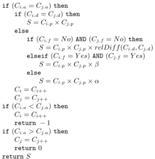
if(Ci.a= Cj.a) then

if(Ci.d= Cj.d) then

S= Ci.p× Cj.p

else

if(Ci.f = N o) AND (Cj.f= N o) then

S = Ci.p× Cj.p× relDif f (Ci.d, Cj.d)

elseif(Ci.f= Y es) AND (Cj.f= Y es)

S = Ci.p× Cj.p× β

else

S = Ci.p× Cj.p× α

Ci= Ci++

Cj= Cj++

if(Ci.a< Cj.a) then

Ci= Ci++

return − 1 if(Ci.a> Cj.a) then

Cj= Cj++

return0 return S

Fig. 3.Algorithm to compute intermediate similarity value.

If the attributes of both the constraints are the same then an intermediate similarity value is calculated by checking the description values. For an exact match between the two constraints (Ci.d = Cj.d), the intermediate similarity

value is obtained by multiplying priority values (Ci.p× Cj.p) . The multiplication

of priority values of both the constraints ensures that a soft constraint with higher priority would secure higher intermediate similarity value.

If the description values are not same then an intermediate similarity value is calculated by considering the flexibility of the constraints. When hard constraints in two profiles do not match, instead of reducing the similarity value to zero, we compute a relative difference between the two corresponding description values of these attributes. For computing the relative difference, a routine relDiff is used. Note that for numeric and alphabetical values of d, separate routines are required to obtain relative differences. Since we are considering hard constraints, our algorithm for relDiff routine adjusts the difference by a factor so that the resulting intermediate similarity value is substantially small.

The parameters α and β are compromise count reduction factors used in a case of compromise match and its usage is elaborated in the next section.

A list of our use case profiles of landlords (LP-1 to LP-6) and Tenants (TP-1 to TP-6) is tabulated in Appendix A. Following example shows how similarity value is obtained when profile TP-1 is matched with profile LP-2.

Intermediate similarity values are computed when each constraint of TP-1 is compared with corresponding constraint of LP-2. One constraint of TP-TP-1 with attribute ‘available’ does not have corresponding attribute match in LP-2 profile. The description values of both the profiles for constraints with attributes

‘bedrooms’ (2 each), ‘rent’ (600· · ·900 and 625) and ‘type’ (apartment each) have an exact match. Whereas for ‘allowSmoke’ attribute, the description values mismatch (yes and no respectively). But both the ‘allowSmoke’ constraints are soft constraints and hence the similarity value is multiplied by an appropriate compromise count reduction factor β.

3

Compromise Match

The concept of soft constraints induces the notion of a compromise match. We define the concept of compromise matching and illustrate its implementation in this section.

As defined earlier, soft constraint indicates participant’s approval to counter-part’s facet value irrespective of match with his/her own facet value. Such soft constraints, in particular, lead to compromise matching between any two profiles in a matchmaking system. A pair of constraints from two profiles said to have a compromise match if, either one or both of the constraints in a comparison are soft constraints and the values of the facets of both the corresponding constraints do not match. In such a case, either one or both participants may compromise with the mismatching value mentioned in the counterpart constraint. Hence we refer to it as a ‘compromise match’.

The ‘allowSmoke’ attribute of the first constraint of the TP-1 profile when compared with the ‘allowSmoke’ constraint of the profile LP-3, it results in an exact match for these constraints. The matching value ‘yes’ for these two constraints yield an exact match. However, when the same constraint from the TP-1 profile is compared with an appropriate constraint of the LP-2 profile, a compromise match emerges. Both the above mentioned conditions are satisfied. A compromise match would also result when the same constraint of TP-1 is compared with a corresponding constraint of profile LP-1.

A compromise match is not an exact match hence a similarity value between corresponding profiles should be reduced. In our matchmaking system, when there is a compromise match between two constraints, an intermediate similarity value (refer algorithm in Fig 3) is reduced by a certain factor. Consider an example of a soft constraint by a landlord, “rent is $700 and can be negotiated” (LP-4) and a tenant’s (buyer’s) soft constraint as “I am ready to pay $500 as rent but can pay more for additional services” (TP-3). These two constraints have a compromise match. As both the participants are ready to compromise with their preferred rent amounts, it is likely that these two participants can reach an agreement. Despite of a difference of $200 these two participants’ willingness to negotiate on rent facet is a prominent factor that increases the likelihood of an agreement between these two participants.

In case of a comparison between the same LP-4 rent constraint with TP-2 rent profile constraint ($600 rent amount and a hard constraint), it is important to note that, only one participant (the landlord) is willing to negotiate. Although the difference in preferred amount is of $100, the likelihood of an agreement

between these two profiles (LP-4 and TP-3) is relatively less than the participants in earlier example (LP-4 and TP-2).

Hence, we conclude that a similarity value in case of a compromise match is influenced by the count (compromise count factor) of participants (one or both) willing to compromise.

We propose two compromise count reduction factors, α and β to reduce an intermediate similarity value, in case of a compromise match. The compromise count reduction factor α is associated with compromise count factor value 1 while the β is associated with compromise count factor value 2. The values of α and β are parameters of our system and are set to less than 1. The algorithm given in the previous subsection to compute the intermediate similarity value S shows how these parameters are used in the calculation. The next section demonstrates effect of different values of α and β on ranking of the matching profiles.

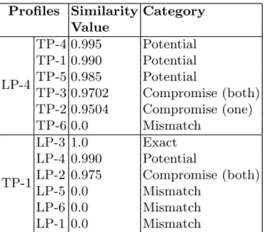
Table 1.Results of Matchmaking. Profiles Similarity Category

Value LP-4 TP-4 0.995 Potential TP-1 0.990 Potential TP-5 0.985 Potential TP-3 0.9702 Compromise (both) TP-2 0.9504 Compromise (one) TP-6 0.0 Mismatch TP-1 LP-3 1.0 Exact LP-4 0.990 Potential LP-2 0.975 Compromise (both) LP-5 0.0 Mismatch LP-6 0.0 Mismatch LP-1 0.0 Mismatch

If a compromise count is one, then there are relatively fewer chances of an agreement as only one participant is ready to compromise. The compromise count reduction factor α represents this case, while the factor β is used when compromise count is two. We set the values of parameters α and β such that a higher similarity value shall be resulted in a compromise match where both participants are ready to compromise and relatively a lower similarity value shall be resulted if only one participant is ready to compromise.

We have implemented the compromise matching in Java and incorporated it in our previous matchmaking system [11] for computing similarity between a set of given profiles. We have applied the system to find the similarity values for all possible combinations for the profiles LP-4 and TP-1 and the result is presented in Table 1. The table also specifies the category of the match between any two profiles Px and Py. The categories are defined as follows:

1. Exact: All constraints of profile Px are present in profile Py and have exact

matches.

2. Potential: Some of the constraints from profile Pxare not present in profile

Py. However, all the remaining constraints of profiles Pxand Py have exact

matching constraints.

3. Compromise: At least one compromise match exists between the con-straints of profile of Px and profile Py. Based on the compromise count

factor we propose two subcategories as

(a) Compromise(both): A compromise match with compromise count fac-tor two.

(b) Compromise(one): A compromise match with compromise count fac-tor one.

4

Compromise Match Trade Off

Let profile PA, PB and PC are three profiles. PA has two soft constraints, PB

has one hard constraint and PC has two soft constraints.

Let M atch1 be a similarity value between PA and PB (single compromise

match). Let M atch2 be a similarity value between PAand PC (two compromise

matches).

It is obvious that user would wish ranking of these matches that comply M atch1 > M atch2.

But when compromise count factor is considered the ranking is not that obvious.

Let M atch3 be a similarity value between PA and PB (single compromise

match) with compromise count factor 1 (only one participant is ready to com-promise, owner of PA in this case). Let M atch4 be a similarity value between

PA and PC (two compromise matches) with compromise count factor 2 (both

participants are ready to compromise).

In this case, one can not easily determine whether M atch3 should be grater than M atch4 or M atch4 should be grater than M atch3. Participants’ choice should be decisive in this trade off.

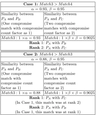
By setting the values of compromise count reduction factors α and β as shown in table 2, we can manipulate ranks in such matchings.

This example illustrates how different values of compromise count reduction factors can be used for ranking matchmaking results according to user prefer-ences.

5

Conclusion

The flexibility supported to participants by the soft constraints leads to compro-mise matching. We have explicitly defined comprocompro-mise matching and identified important aspects associated with it. We have developed a matchmaking system in Java for computing similarity among a set of given profiles. We illustrated

Table 2.Compromise Match and Ranking Case 1: M atch3 > M atch4

α= 0.93, β = 0.95 Similarity between Similarity between PA and PB PA and PC

(One compromise (Two compromise match with compromise matches with compromise count factor as 1) count factor as 2)

M atch3 : 1 ×α = 0.93 M atch4 : 1 ×β × β = 0.9025 Rank1: PA with PB

Rank2: PA with PC

Case 2: M atch4 > M atch3 α= 0.88, β = 0.95 Similarity between Similarity between PA and PB PA and PC

(One compromise (Two compromise match with matches with compromise count compromise count factor as 1) factor as 2)

M atch3 : 1 ×α = 0.88 M atch4 : 1 ×β × β = 0.9025 Rank1: PA with PC

(In Case 1, this match was at rank 2) Rank2: PA with PB

compromise matching using this matchmaking system. We have applied the sys-tem to determine the similarity among seller and buyer profiles that are obtained from an existing e-marketplace. The role of soft constraints in such compromise matches has been elaborated. We proposed and demonstrated the effect of com-promise count reduction factors in ranking of matches.

References

1. Bhavsar, V.C., Boley, H., Lu, Y.: A Weighted-Tree Similarity Algorithm for Multi-Agent Systems in e-Business Environments. Computational Intelligence, 20, 584–602 (2004)

2. Kuokka, D., Harada, L.: Integrating Information via Matchmaking. Journal of In-telligent Information Systems, 6, 261–279 (1996)

3. Liesbeth, K., Rosmalen, P.,Sloep, P.,Kon, M., Koper, R.: Matchmaking in Learning Networks: Bringing Learners Together for Knowledge Sharing Systems. The Nether-lands Interactive Learning Environments, 15(2), 117–126 (2007)

4. Mohaghegh, S., Razzazi, M.R.: An Ontology Driven Matchmaking Process. World Automation Congress, 16, 248–253 (2004)

5. Noia, T. Di., Sciascio, E.Di.,Donini, F.M.,Mongiello, M.: A System for Principled Matchmaking in an Electronic Marketplace. International Journal of Electronic Commerce, 8, 9–37 (2004)

6. Subrahmanian, V. S., Bonatti, P.,Dix, J.,Eiter, T., Kraus,S., Ozcan, F., Ross, R.: Heterogenous Agent Systems. MIT Press, 2000.

7. Sycara, K., Widoff, S.,Klusch, M.,Lu, J.: Larks: Dynamic Matchmaking among Het-erogeneous Software Agents in Cyberspace. Autonomous Agents and Multi-Agent Systems, 5, 173–203 (2002)

8. Veit, D., Mller, J.P.,Weinhardt, C.: Multidimensional Matchmaking for Electronic Markets. International Journal of Applied Artificial Intelligence, 16, 853–869 (2002) 9. Joshi, M.R., Bhavsar, V.C., Boley, H.: Knowledge Representation in Matchmak-ing Applications In Akerkar R., Sajja, P. (eds) Advanced Knowledge based Sys-tems:Models Applications and Research, pp. 29–49, (2010)

10. Joshi, M.R., Bhavsar, V.C., Boley, H.: Matchmaking in P2P e-Marketplaces: Soft Constraints and Compromise Matching In: 12th International Conference on e-Commerce (ICEC 2010) pp. 148–154. (2010)

11. Joshi, M.R., Bhavsar, V.C., Boley, H.: A Knowledge Representation Model for Matchmaking System in Marketplaces, In: 11th International Conference on e-Commerce (ICEC 2009) pp. 362–365. ACM, (2009)

12. Ragone, A., Straccia, U., V.C., Noia, T. Di., Sciascio, E.Di.,Donini, F.M.: Vague Knowledge Bases for Matchmaking in P2P E-Marketplaces, In: 4th European con-ference on The Semantic Web (ECSW-07) pp. 414–428. Springer (2007)

Appendix A: Sample Profiles

A sample list of landlord profiles and tenant profiles obtained from an on-line free local classifieds service available at ‘http://fredericton.kijiji.ca’.

LP-1

<allowSmoke, {no}, No, 1> <available,{Sept-1},No,1> <pets, {no}, No, 1> <rent, {395}, No,1>

<type,{bachelor},No, 1> LP-2

<allowSmoke, {no}, Yes, 1> <bedrooms,{2},No,1> <parking, {1}, No, 1> <rent, {625}, No,1> <type,{apartment},No, 1>

LP-3

<allowSmoke, {yes}, No, 1> <available,{Sept-1},No,1> <bedrooms,{2},No,1> <laundry, {yes}, No, 1> <parking, {2}, No, 1> <rent, {900}, No,1> <type,{apartment},No, 1>

LP-4

<bedrooms,{2},No,1><lease,{year},No,1> <laundry, {yes}, No, 1> <rent, {700}, Yes,1> <type,{apartment},No, 1>

LP-5

<available,{Sept-01},No,1> <bedrooms,{3},No,1> <rent, {600· · ·900}, No, 1> <security,{700},No,1> <type,{apartment},No, 1>

LP-6

<rent, {300}, No,1> <type,{room},No, 1> TP-1

<allowSmoke, {yes}, Yes, 1> <bedrooms,{2}, No, 1> <available,{Sept-1}, No, 1> <type,{apartment}, No,1> <rent, {600· · ·900}, No, 1>

TP-2

<bedrooms, {2}, No, 1> <kids,{yes}, No, 1> <pets,{yes}, No, 1> <rent, {600}, No, 1> <type,{apartment}, Yes,1>

TP-3

<laundry,{yes}, Yes, 1> <pets,{yes}, No, 1> <rent, {500}, Yes, 1> <type,{apartment}, Yes,1> TP-4

<area,{downtown}, No, 1> <available,{Sept-1},No,1> <bedrooms,{2},No,1> <kids,{no}, No, 1>

<laundry, {yes}, No, 1> <pets, {yes}, No, 1> <rent, {800}, Yes, 1> <type,{apartment}, No,1> TP-5

<available,{Sept-1},No,1> <rent, {800}, No, 1> <type,{apartment}, No,1>

TP-6

<available,{Sept-1},No,1> <parking, {1}, Yes, 1> <rent, {500}, No, 1> <type,{bachelor}, No,1>