Biomedical applications of holographic microscopy

Biomedical Applications of Holographic Microscopy

by Ismail Degani

B.S., Computer Science, Cornell University (2005)

Submitted to the Integrated Design & Management Program and

Department of Electrical Engineering and Computer Science

in partial fulfillment of the requirements for the degree of

Master of Science in Engineering and Management and

Master of Science in Electrical Engineering and Computer Science at the

MASSACHUSETTS INSTITUTE OF TECHNOLOGY

June 2018

© Massachusetts Institute of Technology 2018. All rights reserved.

Author . . . .

Department of Electrical Engineering and Computer Science

Integrated Design & Management Program

May 24, 2018

Certified by. . . .

Ralph Weissleder

Professor of Radiology, Harvard Medical School

Thesis Supervisor

Certified by. . . .

Jongyoon Han

Professor of Electrical Engineering and Computer Science

Thesis Reader

Accepted by . . . .

Matthew Kressy

Senior Lecturer

Director, Integrated Design & Management Program

Accepted by . . . .

Leslie A. Kolodziejski

Professor of Electrical Engineering and Computer Science

Chair, Department Committee on Graduate Students

Biomedical Applications of Holographic Microscopy

by

Ismail Degani

Submitted to the Integrated Design & Management Program and Department of Electrical Engineering and Computer Science

on May 24, 2018, in partial fulfillment of the requirements for the degree of

Master of Science in Engineering and Management and Master of Science in Electrical Engineering and Computer Science

Abstract

Identifying patients with aggressive cancers is a major healthcare challenge in resource-limited settings such as sub-Saharan Africa. Holographic imaging techniques have been shown to perform diagnostic screening at low cost in order to meet this clinical need, however the computational and logistical challenges involved in deploying such systems are manifold.

This thesis aims to make two specific contributions to the field of point-of-care diagnostics. First, it documents the design and construction of low-cost holographic imaging hardware which can serve as a template for future research and development. Second, it presents a novel deep-learning architecture that can potentially lower the computational burden of digital holography by replacing existing image reconstruc-tion methods. We demonstrate the effectiveness of the algorithm by reconstructing biological samples and quantifying their structural similarity relative to spatial decon-volution methods. The approaches explored in this work could enable a standalone holographic platform that is capable of efficiently performing diagnostic screening at the point of care.

Thesis Supervisor: Ralph Weissleder

Acknowledgments

First and foremost, I would like to thank the staff and faculty at Center for Systems Biology at the Massachusetts General Hospital for making this research possible. In particular, principal investigators Ralph Weissleder, Hakho Lee, Hyungsoon Im, and Cesar Castro in the Biomedical Engineering Group provided their time, guidance and expertise over many months to bring this work to fruition. I also received generous support from fellows and research assistants in the lab including Phil McFarland, Matthew Allen, Lucas Rohrer, and Divia Pathania, who were all wonderful to work with and incredibly talented.

At MIT, I am very grateful to HST Professor Richard Cohen for offering me a teaching assistantship in his course “Evaluating a Biomedical Business Concept.” This role has not only supported me financially, but also has given me the opportunity to learn and grow as an engineer, scientist, and entrepreneur. I am also grateful to Professor Tonio Buonassisi and instructor Steve Banzaert who awarded me a teaching assistantship for their course “Electronics for Mechanical Systems.” This was an excellent opportunity to sharpen my teaching and coaching skills.

I would like to give the MIT Legatum Foundation a heartfelt thanks for their generous fellowship in my 3rd year of graduate school. Through the fellowship, I met many inspiring entrepreneurs and colleagues with whom I hope to stay lifelong friends. Georgina Flatter, Megan Mitchell, and Julia Turnbull, Reinaldo Normand and the rest of the staff made every effort to champion my work and cultivated a real sense of belonging and community for me at MIT.

I would like to thank Professors Ian Hunter, Amar Gupta, Peter Szolovits, and David Gifford for offering courses that accommodated aspects of my thesis as a final project. I’d also like to thank classmates Suhrid Deshmukh and Hillary Doucette who teamed up with me on these final projects. By doing so they have greatly supported the research presented here. In fact, several key results in this thesis are a direct result of these collaborations.

phases of this project, and for his incisive commentary on new technologies and biomedical innovation. Our conversations have heavily influenced my perspectives in many areas. I also want to thank my friend and colleague Ben Coble for his inspiring designs and illustrations that have meaningfully shaped the direction and character of this project.

I would like to thank the MIT EECS Department for giving me the opportunity to earn a dual master’s degree, and also for graciously accepting me into their PhD program. I am very excited about continuing my journey of discovery and learning at MIT. I also want to thank IDM Co-Directors Steve Eppinger, Warren Seering and Matthew Kressy for opening the doors of MIT to me, which has forever changed my life’s trajectory and will be an enduring source of pride for years to come.

Lastly, I am grateful to my parents Nafisa & Ibrahim, my brother Isaac, and the rest of my family and friends who have supported me throughout this journey with their unwavering kindness and understanding.

Contents

1 Introduction 15

2 Background 17

2.1 Prior Attempts . . . 17

2.2 Digital Diffraction Diagnostic (D3) . . . 18

2.3 Unit Economics . . . 18

2.4 Progress . . . 18

2.5 Assessed Needs . . . 19

2.5.1 Connectivity . . . 20

2.5.2 Integrated Standalone Device . . . 20

3 Digital Holography and Reconstruction 23 3.1 Working Principle of Lensless Holography . . . 23

3.2 Holographic Transfer Function . . . 24

3.3 Phase Retrieval . . . 27

4 Hardware Design and Fabrication 31 4.1 Digital Diffraction Diagnostic . . . 31

4.2 Smartphone (iPhone) D3 Prototype . . . 32

4.2.1 Methods and Materials . . . 32

4.2.2 Design Drawbacks . . . 33

4.3 ARM Cortex M0 Prototype . . . 34

4.4 Raspberry Pi D3 Prototype . . . 36

4.4.1 Kinematic Couplings . . . 37

4.4.2 Sliding Tray Design . . . 37

4.4.3 Optical Post Design . . . 37

4.4.4 Electrical PCB Design . . . 38

4.4.5 UI Design . . . 40

4.4.6 Methods and Materials . . . 41

4.4.7 Deep Convolutional Networks . . . 41

5 Synthetic Hologram Classification 43 5.1 Repurposed MNIST Classifier . . . 43

5.1.1 Results . . . 44

5.2 Isolated Diffraction Simulation . . . 45

5.2.1 Results . . . 46

5.3 U-net Segmentation (Undiffracted) . . . 47

5.3.1 Results . . . 49 5.4 Diffraction Segmentation . . . 50 5.4.1 Results . . . 50 5.5 Discussion . . . 51 6 U-Net Reconstruction 53 6.1 Dataset . . . 53 6.1.1 Phase Recovery . . . 54

6.1.2 Data Pre-processing and Augmentation . . . 54

6.1.3 Training, Validation and Test Split . . . 55

6.2 Network Architecture . . . 55

6.2.1 Independent U-Nets for 𝐼𝑟𝑒 and 𝐼𝑖𝑚 . . . 57

6.2.2 Modifications to U-Net . . . 57

6.2.3 PReLU: Parametrized ReLU . . . 57

6.2.4 U-Net Hyperparameters . . . 58

6.3.1 Mean-square error . . . 59

6.3.2 Structural Similarity Index Metric (SSIM) . . . 59

6.3.3 Loss Functions and Optimizer . . . 59

6.4 Results . . . 60 6.4.1 Hyperparameter Optimization . . . 60 6.4.2 Training Epochs . . . 61 6.4.3 Qualitative Performance . . . 62 6.5 Future Directions . . . 63 7 Conclusion 65 7.1 Drawbacks of Deep Learning . . . 66

7.2 Impact . . . 66 A Holographic Reconstruction with Iterative Phase Recovery in Python 69

List of Figures

2-1 D3 Workflow Photo Credits: Ben Coble, Women’s Health Mag., Biogen Inc. 18

2-2 D3 Cost per Test [11] . . . 19

2-3 Local technician training Photo Credit: Alexander Bagley . . . 20

2-4 Five-Year Research and Development Timeline . . . 20

3-1 Digital Holographic Imager [27, 7] . . . 24

3-2 Raw Hologram (Left) and Reconstruction (Right) . . . 24

3-3 A Seemingly Complicated Reconstruction . . . 25

3-4 Holographic Transfer Function . . . 25

3-5 Numerical Forward Propagation at 𝜆 = 405𝑛𝑚 . . . 26

3-6 Twin Image Problem - Latychevskaia et al [16] . . . 27

3-7 Object Support Generation . . . 28

3-8 Convergence of Phase Recovery Step . . . 29

4-1 D3 Binding and Reconstruction - Im et al [11] . . . 32

4-2 iPhone Prototype . . . 33

4-3 D3 HPV Imaging Unit CAD Model . . . 34

4-4 D3 HPV Imaging Unit . . . 35

4-5 D3 B-Cell Lymphoma Platform CAD Rendering and Device Photo . 36 4-6 Kinematic Coupling CAD and Photo . . . 37

4-7 Sliding Tray CAD . . . 38

4-8 Optical Post Assembly . . . 39

4-9 Electrical Circuit Board . . . 40

4-11 Reconstruction via Convolutional Neural Network . . . 42

5-1 Cell-binding compared to the MNIST Dataset . . . 44

5-2 Two-layer CNN Performance: 97.61% Accuracy . . . 45

5-3 Output of first convolutional layer . . . 45

5-4 Isolated Diffraction Dataset . . . 46

5-5 Performance of Diffraction Classifier . . . 47

5-6 Simulated “Ensemble” Dataset . . . 48

5-7 Custom 3-Layer U-Net Architecture . . . 48

5-8 U-Net Training Error . . . 49

5-9 U-Net Segmentation Map by Epoch . . . 49

5-10 Diffraction of Ensemble Dataset . . . 50

5-11 Accuracy Metrics of Predictions . . . 51

5-12 Diffraction Reconstruction by U-Net on a Diffracted Ensemble . . . . 51

6-1 Lymphoma (DAUDI) Cell Line . . . 54

6-2 Data pre-processing . . . 55

6-3 Six-Layer U-Net Architecture . . . 56

6-4 ReLU (left) vs PReLU (right) - He et al [10] . . . 58

6-5 SSIM of Test Set Predictions: ReLU (left) and PReLU (right) . . . . 61

6-6 Prediction Evolution by Epoch . . . 61

6-7 Train / Validation Loss by Epoch . . . 62

6-8 Qualitative U-Net Performance . . . 63

List of Tables

4.1 Cost Breakdown of D3 HPV Imaging Unit . . . 35

4.2 Optical Post Components . . . 39

6.1 D3 Image Capture Parameters . . . 54

6.2 Samples in each dataset partition . . . 55

6.3 U-Net Hyperparameters . . . 58

Chapter 1

Introduction

The worldwide adoption of smartphones has yielded economies of scale which have caused the prices of many integrated sensors to plummet. In particular, high-resolution 10 megapixel CCD camera modules with pixel sizes as small as 1.2 um can now be readily purchased for $10-$15 USD (Source: Digikey). This is a remarkable trend, and it is fueling a myriad of research and development efforts in the biomedical domain [31, 33].

At the same time, the world’s healthcare challenges are dire and growing. The AIDS epidemic in sub-Saharan Africa has led to a high prevalence of cancers such as aggressive B-cell lymphoma, whose incidence has continued to rise despite the in-troduction of anti-retroviral therapies [2]. In resource-limited settings, these cancers often go undiagnosed due to a dearth of trained pathologists (less than 1 per mil-lion patients vs. 30 per milmil-lion in developed countries [18]). With an insufficient capability to run diagnostic tests, precious windows of intervention are often missed. Therefore there is a significant clinical need for a low-cost diagnostic that can ac-curately identify patients with aggressive cancer who require immediate therapy. If malignant strains can be identified early on, many of these cases are curable even in low-income countries. [12].

A potentially game-changing technique in the area of low-cost diagnostics is lens-less digital holography (LDH). It has been used extensively across microbiological applications ranging from cancer screening to bacterial identification [31, 22, 21].

Holography itself is not new: Dennis Gabor published the original 1948 paper in Nature [5] and won the Nobel prize for it in 1971. In subsequent years, holography remained a relatively niche technology without many practical applications [20] due to the fine resolution required to capture interference fringes. Now, with recent ad-vances in high-resolution CMOS and CCD camera sensors, LDH is emerging as a viable alternative to traditional microscopy due to its low cost and high portability. By leveraging computational techniques, LDH provides high-resolution images with a very wide field-of-view (>24mm2). In a biological context, this translates to

simulta-neous imaging of between 10,000 and 100,000 cells in a single snapshot. LDH is also able to recover the refractive index of objects such as cells or bacteria in an aqueous sample [22], which makes it a powerful platform for running diagnostic tests. Finally, because LDH can capture phase information, it is able to image transparent objects. This is a powerful advantage because it eliminates the need for staining and other biological labeling methods (i.e. “label-free” detection).

This thesis will explore the challenges associated with designing and deploying an LDH-based diagnostic screening system. Chapter 2 will give an overview of the context of the project and its motivation. Chapter 3 will provide a thorough back-ground on the working principles of the holographic method, and Chapter 4 will discuss the design and construction of prototypes that can capture holograms at low cost. Chapters 5 and 6 will focus on novel algorithms that can potentially optimize the computationally expensive image reconstruction process. The ultimate goal is to build a system that can operate in resource-limited settings with low connectivity and still provide accurate and rapid testing.

Chapter 2

Background

The research described in this thesis has been done in the context of NIH grant CA202637-01, which is a multi-year initiative to address the problem of lymphoma in Africa. This chapter will summarize the ongoing developments in Botswana, where a clinical trial utilizing digital holographic imaging is scheduled to commence in 2018/2019.

2.1

Prior Attempts

The standard approaches to cancer screening include methods such as flow cytometry and various forms of microscopy. These traditional methods are very accurate, how-ever they are not feasible to implement and scale in a resource limited setting. There are also low-cost techniques such as paper diagnostics [23] that provide an acceptable price point. However they tend to be lower resolution, and are not of suitable qual-ity for providing a cancer diagnosis. While research in this area is vibrant, there is currently no fully implemented solution that meets both the stringent standards of oncology screening and the price point of a resource limited environment.

2.2

Digital Diffraction Diagnostic (D3)

The “D3 platform” [11] is a diagnostic system that aims to meet the needs of cancer screening in the developing world by delivering results rapidly and cost-effectively. The technology was developed at the Massachusetts General Hospital (MGH). It consists of a portable device and cloud-based analysis server. A key aspect of the device is that it is designed to be operated by lab technicians rather than pathologists. This results significant cost savings and can also alleviate the strain on oncology specialists in low-income areas. Fig. 2-1 illustrates a simplified workflow of the screening process.

Figure 2-1: D3 Workflow

Photo Credits: Ben Coble, Women’s Health Mag., Biogen Inc.

2.3

Unit Economics

The estimated cost per test are given in Fig. 2-2. The system provides an unprece-dented cost savings over traditional cancer screening methods by utilizing low-cost sensors and eliminating all manual assessment done by a pathologist.

2.4

Progress

Progress to date includes the iterative development of three fully operational proto-types of the D3 imaging system and plastic cartridges for assays. These were de-veloped at MIT under supervision of the MGH Biomedical Engineering group. Two

Figure 2-2: D3 Cost per Test [11]

early prototypes were shipped to Botswana in May 2016 where initial pre-clinical data was gathered. Three MGH partner hospitals will participate in the 2018/2019 prospective trial:

1. Princess Marina Hospital, Gaborone: the largest public hospital in Botswana. 2. Gabarone Private Hospital: the largest private hospital in Botswana.

3. Nyangabwe Referral Hospital, Francistown: a principal oncology center in North-ern Botswana

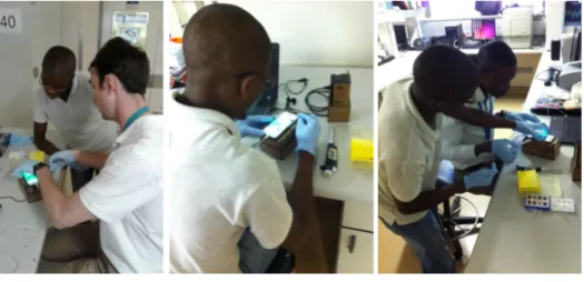
Fig. 2-3 shows a session where local technicians are trained to run lymphoma screens on patient samples. The clinical trial will enroll 200 patients across 30 rural villages [30].

Pending a successful trial, the device is expected to enter the manufacturing phase by 2020. Fig. 2-4 gives an outline of the expected timeline for commercialization.

2.5

Assessed Needs

During the pre-clinical test phase, several issues emerged which this thesis aims to address at the hardware and software level.

Figure 2-3: Local technician training

Photo Credit: Alexander Bagley

Figure 2-4: Five-Year Research and Development Timeline

2.5.1

Connectivity

The biggest issue was broadband network connectivity, which is required to transmit image data to a host GPU server for analysis. An intermittent or weak connection can result in transmission errors which prevents the clinician from providing an onsite diagnosis. Slow connections can also be an impediment because the 5-10 megapixel images must be transmitted in a lossless format for a proper analysis. Connectivity issues are recurrent in virtually all places where low-cost diagnostics are necessary, therefore addressing them is of high importance.

2.5.2

Integrated Standalone Device

Using a smartphone-based holographic companion system as originally described in PNAS [11] presents several technical challenges which are described in Chapter 4.

Aside from these, there is also a human-error factor that is amplified when multiple hardware components need to be orchestrated by technicians. As such, a fully inte-grated device that standardizes all internal components was deemed optimal. In this design, configurability is minimized and the user is given clear instructions by the software interface throughout the screening process.

Chapter 3

Digital Holography and

Reconstruction

Digital in-line holography [31, 11] is an emerging technique that is gaining prominence in the area of clinical pathology. This chapter gives an overview of digital reconstruc-tion, which is central to holographic imaging. Much of the published literature on this subject [14, 3] is relatively abstract and can obscure the basic fundamentals of the algorithm. The aim of this chapter is to provide a simple step-by-step explanation of in-line holographic reconstruction with an abundance of figures, illustrations, and code samples in order to explain the key points of the method.

3.1

Working Principle of Lensless Holography

In lens-free digital holographic microscopy (LDHM), biological samples are often placed directly on top of an optical sensor array (or very close to it) in order to maximize the instrument’s field of view. Usually this camera sensor is a complemen-tary metal oxide semiconductor (CMOS) or charged-couple device (CCD) array, as shown in Fig. 3-1. Light from a high-power LED passes through a pinhole, which illuminates the sample with substantially coherent monochromatic light.

As the name LDHM suggests, diffraction pattern created by objects in the sample are directly captured by the camera sensor without the aid of lenses. An iterative

Figure 3-1: Digital Holographic Imager [27, 7]

algorithm must “reconstruct” an estimate of the true image via spatial deconvolutions [14]. The algorithm used to accomplished this is described in detail in the following sections. Lensless holography yields a myriad of advantages in microscopy including simple design, high resolution, and a wide field-of-view [32, 19].

3.2

Holographic Transfer Function

An example of a raw holographic image and its reconstruction is given in Fig. 3-2. This is a cluster of polystyrene microbeads that are approximately 6𝜇𝑚 in diameter.

Figure 3-2: Raw Hologram (Left) and Reconstruction (Right)

The light scattered by microscopic objects is quite analogous to the ripples created by pebbles dropped in a pond. Note how their diffraction patterns can overlap and interfere with each other. At first glance, it may appear very difficult to automatically “de-blur” such an image, or reconstruct the pebbles that created each set of ripples.

Fortunately, since light obeys very precise physical laws, it is possible to efficiently model and reverse its paths digitally. This allows for the reconstruction of impossibly crowded samples like Fig. 3-3

Figure 3-3: A Seemingly Complicated Reconstruction

To undo the blurring effects of optical diffraction, holographic image reconstruc-tion relies on the transfer funcreconstruc-tion of free-space propagareconstruc-tion, illustrated in Fig. 3-4. As shown, 𝑧 is the axis representing the perpendicular distance from the sample to the camera sensor, 𝜆 is the wavelength of light emitted by the LED, and (𝜁, 𝜂), (𝑥, 𝑦) form the coordinate systems of the hologram and object planes, respectively.

Figure 3-4: Holographic Transfer Function

The impulse response and transfer function of free-space propagation are given in equations 3.1 and 3.2 respectively [14].

𝑔𝑏𝑝(𝜁, 𝜂) = 1 𝑖𝜆 exp[︁𝑖𝑘(𝑧2_{+ 𝜁}2_{+ 𝜂}2₎1/2]︁ 𝑧2_{+ 𝜁}2_{+ 𝜂}2 (3.1) 𝐺𝑏𝑝(𝑓𝜁, 𝑓𝜂) = 𝑒𝑥𝑝 [︂ 𝑖𝑘𝑧(︁1 − 𝜆2𝑓_𝜁2− 𝜆2_𝑓2 𝜂 )︁1/2]︂ (3.2) Eq. 3.1 is also known as the Rayleigh-Somerfield diffraction kernel, and with it one can numerically compute the propagation of a wavefront in space. To obtain the forward propagation kernel 𝐺𝑓 𝑝, we simply take the reciprocal of 𝐺𝑏𝑝:

𝐺𝑓 𝑝(𝑓𝜁, 𝑓𝜂) = 𝑒𝑥𝑝 [︂ −𝑖𝑘𝑧(︁1 − 𝜆2𝑓_𝜁2− 𝜆2_𝑓2 𝜂 )︁1/2]︂ (3.3)

The above formulation is used to backpropagate the optical intensity pattern recorded at the hologram plane ℎ to the object plane 𝑜 and resolve the objects. This is accomplished by convolving the captured hologram ℎ with 𝑔𝑏𝑝. In practice, this is

performed by multiplying the Fourier transform (𝐻) of ℎ with 𝐺. Recall that by the convolution theorem, the convolution of two functions 𝑎 and 𝑏 is equal to the product of their Fourier transforms (Eq. 3.4).

ℱ {𝑎 * 𝑏} = ℱ {𝑎}ℱ {𝑏} (3.4)

Taking the inverse Fourier transform of both side, we obtain:

𝑎 * 𝑏 = ℱ−1{ℱ {𝑎}ℱ {𝑏}} (3.5) Applying 3.5 to our target functions:

𝑂(𝑥, 𝑦) = 𝑔(𝜁, 𝜂) * ℎ(𝜁, 𝜂) = ℱ−1{𝐺(𝑓𝜁, 𝑓𝜂) · 𝐻(𝑓𝜁, 𝑓𝜂)} (3.6)

Similarly, one may forward-propagate any simulated intensity pattern at the object plane by convolving with 𝐺𝑓 𝑝, as shown in Fig. 3-5. This ability to generate holograms

will become important in later chapters when neural networks are trained on simulated data.

Figure 3-5: Numerical Forward Propagation at 𝜆 = 405𝑛𝑚

Alternative diffraction kernels such as the Fresnel approximation for paraxial beams of light, or the Fraunhofer far-field approximation [4] may also be substituted to generate forward-propagated holograms.

3.3

Phase Retrieval

The workhorse of inline holographic reconstruction is the deconvolution of Eq. 3.6. However an additional iterative error reduction step is needed to combat what is known as the “Twin Image Problem,” [8]. Performing only the naïve deconvolution of Eq. 3.6 can lead to two objects superimposed on each other: the true object, and an erroneous out-of-focus copy that is mirrored in both the x and y axes. These images are illustrated in Fig. 3-6.

Figure 3-6: Twin Image Problem - Latychevskaia et al [16]

Several iterative and non-iterative methods have been proposed to eliminate the twin image problem [28]. The method employed throughout this thesis is the “object support generation method,” which involves (1) generating an estimate of the object boundary from the naïve deconvolution, and (2) iteratively computing phase of the object that minimizes the error of the empty space outside the object’s boundary. This can be restated as finding the phase values that minimize the intensity of the diffraction ripples that occur outside an object’s determined boundary.

Fig. 3-7 outlines the steps to create an support boundary. The first step performs the naïve deconvolution of Eq 3.6. Clearly there are still ripple artifacts remaining around each object. A sliding standard deviation filter followed by a thresholding operation creates the binary mask shown at the very right: this is the object support.

Figure 3-7: Object Support Generation

Particularly in biomedical application involving cell samples and microbeads, objects are likely to be convex ellipsoids. This information can be exploited to further smooth the object masks using image dilation and erosion operations. Note that this method can also serve to eliminate objects that are unwanted, such as the faint hologram that is highlighted in red. Often dust and debris can be eliminated by an appropriate choice of threshold.

Once an object boundary has been defined, the Gerchberg-Saxton [6] error mini-mization algorithm iteratively eliminates the unwanted ripples by altering the phase of the object inside the boundary. The algorithm works as follows:

1. Apply the object support mask to the 𝑖𝑡ℎ _{reconstruction and adjust it by the}

phase of the previous reconstruction.

2. Forward-propagate the adjusted reconstruction to the hologram plane 𝐻. 3. Adjust the input hologram with the new phase information held by the adjusted

hologram of step (2).

4. Backpropagate the adjusted hologram of step (3) to the object plane 𝑂 and obtain the 𝑖 + 1𝑡ℎ _{reconstruction.}

Repeat until converged.

The full implementation of this algorithm can be found in Appendix A. In practice, it is found to converge to minimum ripple outside the object boundary after 10-30 iterations. This convergence is illustrated in Fig. 3-8.

Figure 3-8: Convergence of Phase Recovery Step

After reconstruction and iterative phase retrieval, the image can be readily seg-mented and analyzed via simple techniques such as Maximal Stable Extremal Regions (MSER) [17], or more advanced methods such as a region-proposal network (RPN) that utilizes a neural network architecture (R-CNN) [24].

Chapter 4

Hardware Design and Fabrication

With an understanding of the principle of holography and holographic reconstruction from the previous chapter, we can now proceed to describe our experimental setup. This chapter elaborates on the design and construction of several physical prototypes that were used to capture holographic intensity data for analysis.

4.1

Digital Diffraction Diagnostic

The “D3 platform” [11] combines holographic imaging with bead-binding immunoas-says in order to perform diagnostic screening. Figure 4-1 illustrates the working principle of the technology:

First, antibody-coated beads are constructed to selectively bind to specific surface markers on cells of interest. The sequence 𝐴1 → 𝐴2 illustrates this binding. By identifying and counting the “bead-cell complexes” (𝐴2), one can obtain an accurate quantitative readout for screening purposes.

The caveat is that diffraction patterns 𝐵1 → 𝐵2 are captured, instead of easily discernable brightfield images. To count the bead-cell complexes, a full reconstruction is necessary. This is shown in 𝐶1/𝐶2, where the cells and beads now substantially match their brightfield counterparts 𝐴1/𝐴2.

While the D3 was designed to achieve specific goals in oncology, its imaging prin-ciple is no different than that of any standard holographic system. Therefore the

Figure 4-1: D3 Binding and Reconstruction - Im et al [11]

following device designs could be used in any application involving holographic mi-croscopy.

4.2

Smartphone (iPhone) D3 Prototype

An initial prototype was designed to use an iPhone as the camera sensor of the holographic system. The intent was to capitalize on the ubiquity of smartphones and eliminate the most expensive components of the system: the camera sensor, image processing hardware, data storage, and connectivity components such as a WiFi module.

4.2.1

Methods and Materials

The iPhone prototype was fabricated primarily by laser-cutting 1/8" medium-density particle fiberboard (MDF). A 3D-printed iPhone dock is epoxied to the top surface, and the device’s optics are held in place by a Thorlabs optical cage assembly.

Fig. 4-2 presents several views of this device, and illustrates how the iPhone is seated at the top of the unit. Due to the relatively low tolerances of the laser-cut and 3d-printed components, adjustment screws needed to be added so that optical calibration could be done on-the-fly.

Figure 4-2: iPhone Prototype

4.2.2

Design Drawbacks

The smartphone methodology was successfully used to detect cervical cancer; de-tails are published in PNAS [11]. However, this hardware design has some notable drawbacks:

1. Smartphone camera sensors are already fitted with a complex tube lens, which stipulate that the holographic system include an additional lens to reverse its effects. Introducing a lens carries with it additional cost and alignment issues that counteract the advantages of a lensless holographic system.

2. Smartphone models generally become obsolete in a 1-3 year time horizon. Newer models nearly always have different form factors and API’s which would require both hardware and software modifications to a holographic companion system. This constant maintenance burden would hamper the development of the prod-uct and present major challenges for regulatory approval.

4.3

ARM Cortex M0 Prototype

A second device was built which mitigates some of the aforementioned issues experi-enced by the iPhone prototype. This device was used to detect human papillomavirus (HPV) and was designed to be a compact and portable companion to a PC or laptop computer. The camera sensor was a 5 megapixel CMOS module, which was designed to send images to a host PC over USB 2.0. The CAD model of this unit is shown in Fig 4-3

Figure 4-3: D3 HPV Imaging Unit CAD Model

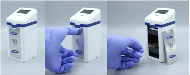
A cost breakdown is given in Table 4.1. These costs are exceedingly low for an optical diagnostic device. When economies of scale are taken into account, the final cost would likely decrease further still. Finally, if the image reconstruction is executed on a GPU server, the total image capture and analysis time could be shortened to minutes. Figure 4-4 illustrates how a sample is loaded into the device.

Component Cost ($ USD) CMOS Camera Sensor 40 1A high-power UV LED 40 OLED screen display 7 Cortex-M0 Microcontroller 1 Optical Components 20 Housing & Misc 10

Total 118

Table 4.1: Cost Breakdown of D3 HPV Imaging Unit

Figure 4-4: D3 HPV Imaging Unit

4.3.1

Methods and Materials

The low-power imaging unit is equipped with a 1.4 A high-power 625-nm LED (Thor-labs) heat-sinked by a metal printed circuit board (PCB) and a custom machined aluminum holder. A 220-grit optical diffuser (DGUV10, Thorlabs) is positioned be-tween the LED and a 50 𝜇𝑚 pinhole (Thorlabs). Optical components are aligned by machined acrylonitrile butadiene styrene (ABS) mounts. Images are captured using a monochromatic 5 megapixel complementary metal-oxide-semiconductor (CMOS) im-age sensor (On-Semiconductor) mounted on a USB 2.0 interface board (The Imaging Source). The pixel size is 2.2 𝜇𝑚 and the field of view is 5.7 x 4.3 𝑚𝑚2_{. Image}

data is transferred from the camera to a companion PC (Dell). An integrated 128x32 monochrome OLED Display (Wise Semiconductor) provides a real time view of sys-tem status, and a momentary switch controls the LED. Images can be directly trans-ferred via USB to a PC or laptop computer using the software package IC Capture

(Imaging Source). They are then forwarded to a cloud-based GPU server for analysis. The unit is powered by a regulated 5V, 15W adapter (Meanwell). The device housing is 3d-printed in white photopolymer resin (Formlabs), and the machined-aluminum door is fastened with 1/8 inch neodymium disc magnets (Grainger). The diffraction chamber is fabricated with black photopolymer resin (Formlabs) and is light-proofed using flocking papers (Edmund Optics). The dimensions of the hardware unit are 65mm (L) x 65 mm (W) x 140 mm (H) and the overall weight is 0.6 kg.

4.4

Raspberry Pi D3 Prototype

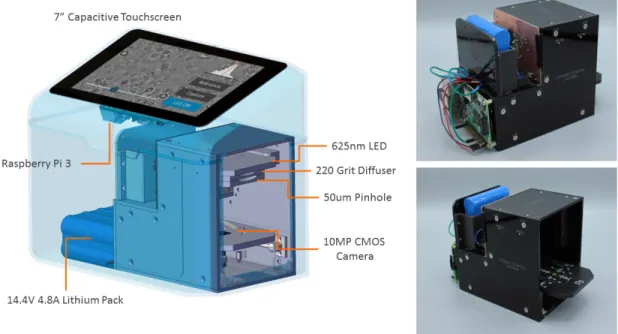
A fully standalone holographic system was built to allow for a streamlined user expe-rience and minimize compatibility issues with external PC’s. The unit was equipped with a raspberry PI and had a custom touchscreen user interface for a technician to control the image capture process. A CAD model of this prototype is shown below.

4.4.1

Kinematic Couplings

To improve the user experience, kinematic couplings [9] were implemented to change optical components such as the LED and pinhole. For a given assay, holographic parameters such as wavelength, pinhole size, and z-height often need to be adjusted in order to obtain optimal images. Having magnetic couplings that can be easily clipped on or off makes the device far more versatile than a standard optical cage which must be dismantled in order to reconfigure.

Figure 4-6: Kinematic Coupling CAD and Photo

4.4.2

Sliding Tray Design

Several iterations of sample loading subsystem were attempted. The first was a sliding tray operated by a stepper motor, shown in Fig. 4-6.

The primary drawback of this system is that the alignment of the camera and LED are prone to change slightly between image captures due to the movement.

4.4.3

Optical Post Design

A simpler design using off-the shelf optical fixtures and clamps was also developed. This design requires manual loading, but can be assembled with minimal machining and 3-d printing, using the parts specified in Table 4.2

Figure 4-7: Sliding Tray CAD

4.4.4

Electrical PCB Design

A custom PCB was designed with simple power management circuitry. The unit is operable either by a lithium battery pack or by wall power. A constant current LED driver (RCD-24-1.00, Recom Inc) powers the high-current LED and an isolated DC-DC converter (PDQ30-Q24-S5-D, CUI Inc) powers the raspberry pi and CMOS

Figure 4-8: Optical Post Assembly

Component Manufacturer Model

CMOS Camera Sensor Imaging Source DMM 24UJ003-ML 1A high-power UV LED Thorlabs M405D2

Optical Post Thorlabs TR100/M

Optical Post Holder Thorlabs PH1

Post Clamp Thorlabs PMTR/M

Diffuser Thorlabs DGUV10-220

Precision Pinhole Thorlabs P50H Table 4.2: Optical Post Components

camera sensor. The total power consumed by the unit is approximately 8 Watts. The Eagle schematic and board files for this PCB are available at the following

Figure 4-9: Electrical Circuit Board GitHub Repository:

https://github.com/deganii/d3-pcb

4.4.5

UI Design

The Raspberry pi operating system “Raspian Stretch” is based on Debian linux 16.04. This made it possible to construct a user interface in a high-level language, rather than C/C++ which would be required on an embedded system.

A user interface was designed in Python 3.5 using the Kivy 1.10 framework. Using this interface, a technician is able to capture a sample and upload it wirelessly to an analysis server in just 2-3 taps.

Figure 4-10: D3 User Interface

The user interface implementation is available at the following GitHub Repository: https://github.com/deganii/d3-ui

4.4.6

Methods and Materials

The integrated imaging unit is equipped with a 1.4A high-power 625-nm LED (Thor-labs) heat-sinked by a metal printed circuit board (PCB) and a custom machined aluminum holder. A 220-grit optical diffuser (DGUV10, Thorlabs) was positioned between the LED and a 50 𝜇𝑚 pinhole (Thorlabs). Optical components were aligned by machined acrylonitrile butadiene styrene (ABS) mounts. Images were captured using a monochromatic 10 megapixel complementary metal oxide semiconductor sen-sor (CMOS; On-Semiconductor) mounted on a USB 3.0 interface board (The Imaging Source).The pixel size is 2.2 𝜇𝑚 and the field of view is 5.7 x 4.3 𝑚𝑚2_{. Image data}

is transferred from the camera to a Raspberry Pi 3.0 (Broadcom BCM2837 SoC) running Debian Linux. An integrated 7" display (Raspberry PI Foundation) pro-vides a real-time view of holographic data, and a touch-screen user interface captures and saves data. Images can be directly transferred via WiFi to a cloud-based GPU server for analysis. The unit is powered by a regulated 18V, 60W adapter (Mean-well) and will run continuously for approximately 6 hours when powered by an 8-cell, 14.8V/4.8Ah Li+ battery pack (UltraLife UBBL26). The device housing was fab-ricated with photopolymer resin (Formlabs), and the machined-aluminum door was fastened with 1/8 inch neodymium disc magnets (Grainger). The diffraction chamber was fabricated using opaque 1/8 inch acrylic sheets (laser ablation) and was light-proofed using flocking papers (Edmund Optics). The dimensions of the hardware unit are 205 mm (L) x 120 mm (W) x 175 mm (H) and the overall weight is 1.4 kg.

4.4.7

Deep Convolutional Networks

Once the requisite hardware was built and assembled, image data could be acquired and transmitted to a centralized cloud server for processing. As described in chap-ter 3, holographic reconstruction with phase recovery is a computationally intensive operation. In practice, it requires a dedicated GPU server to process the data in a reasonable timeframe. As a result, the D3 system is difficult to use in field settings where WiFi connectivity may be slow or intermittent. For the remainder of this

thesis, we attempt to mitigate this problem by leveraging deep neural networks. Deep convolutional neural networks (CNN’s) have been shown to learn highly complex patterns relative to previous approaches [15]. Given the computational bur-den of holographic reconstruction, it is meaningful to ask whether a CNN can be taught to fully reconstruct objects that are enshrouded by optical diffraction. More concretely, the goal is to learn the transformation of Fig. 4-11 in order to output readily countable cells and micro-beads. A neural network that performs this task may be computationally expensive to train; however it is hoped that once trained, the network will be capable of fast feed-forward transformations that far exceed what is possible with the current state-of-the-art. The next two chapters will explore this idea in greater detail.

Chapter 5

Synthetic Hologram Classification

This chapter is structured as a series of experiments that attempted to leverage best practices in neural network architectures to solve small challenges on the path toward learning the diffraction reconstruction transfer function.

Prior to working with biological datasets containing noise and debris, fully syn-thetic datasets were analyzed. The intuition was that simulated holograms with controllable characteristics would yield a higher probability of incremental successes that could built upon. For example, the problem of diffraction classification can be broken down into two independent tasks: (1) image segmentation, and (2) individual object classification. Each of these has different challenges that may be explored more effectively with tailored, simplified datasets.

We employ canonical 2 and 3 layer convolutional neural networks with multiple fully connected layers, and also begin experimenting with a “specialist” architecture U-Net that is designed to solve specific problems relevant to image segmentation.

5.1

Repurposed MNIST Classifier

It is worth questioning whether or not a CNN can effectively classify a cell-bead bind-ing event, which is an important detection mechanism of the D3 (see section 4.1). This requires learning rotational invariance, which unlike translational invariance is not a “natural” capability of a convolutional layer. To confirm this, we attempted to

package the problem as an MNIST classification task. We generated 60,000 training examples and 10,000 test examples of random binding events to match the structure and size of MNIST. Cells and beads were constructed to have matched pixel diam-eters to actual cells (5-7 𝜇𝑚), and the distribution of binding occurrences was also made identical to empirical data. About 50% of the cells were left “unbound,” and the remaining were constructed with 1-5 beads at random non-overlapping orienta-tions. This resulted in a total of six possible classification labels. We then trained an MNIST classifier on this dataset. Fig. 5-1 illustrates this dataset and the intuition behind this strategy: the MNIST digits bear resemblance to the “hieroglyphs” of dif-ferent cell-bead combinations. We hoped to leverage a stable and performant CNN to confirm basic operation before addressing the more challenging aspects of diffraction reconstruction.

Figure 5-1: Cell-binding compared to the MNIST Dataset

5.1.1

Results

A 2-convolutional layer network with 2 fully connected layers was trained using the Adam Optimizer with a learning rate of 0.001. This architecture was shown to achieve 99.2% test accuracy on MNIST. The network was run for 20 epochs on the simulated cell-binding training set, and managed to achieve 97.61% accuracy on the correspond-ing test set.

Because convolutional layers “sweep across” an image to produce activations, they do not have any intrinsic mechanism of learning rotations. Therefore, it is worthwhile to speculate on how this network might be learning rotational invariance. To explore

Figure 5-2: Two-layer CNN Performance: 97.61% Accuracy

this, we visualize the outputs of the first convolutional layer in Fig. 5-3. It appears that this convolution output layer has “thickened” the cell walls of the input. Perhaps the network is attempting to homogenize all rotational variants into a single thickness parameter. It could then make a decision solely based on this and avoid the rotational issue altogether.

Figure 5-3: Output of first convolutional layer

With the success of this basic classifier, we attempt to discover whether the same convolutional architecture is capable of learning diffraction.

5.2

Isolated Diffraction Simulation

Optical diffraction can be expressed as a convolution integral, and several methods exist to compute this transfer function. [14] Here we implement the Fresnel

propa-gator, which simulates the effect of diffraction on each simulated cell of our initial dataset. We process the diffraction using simulated light at wavelength 𝜆 = 405𝑛𝑚, at a z-distance of 0.2𝑚𝑚, and with a pixel resolution of 1.2𝜇𝑚. These conditions are substantially similar to what is actually generated by the holographic hardware (D3) whose images we ultimately aim to process. Fig. 5-4 is an illustration of this transfer function applied to a sample of simulated cells.

Figure 5-4: Isolated Diffraction Dataset

With this diffracted dataset in hand, we are ready to retrain our network to classify simplified, isolated cells. As shown in Figure 5-4, a human observer can easily discern the difference between unbound and bound states. The unbound cell exhibits a distortion-free diffraction pattern which is clearly distinct from the other patterns. However, as the number of bound beads increases, it becomes more difficult to classify the cell.

5.2.1

Results

Using the MNIST network, we were unable to achieve better than 75-80% test accu-racy on the diffracted datasets. Convolutional filters with greater dimensions (10, 15, 20 pixels) were tried to give each filter a greater receptive field. This was done in an attempt to counteract the spatial “spreading” effect of diffraction. When this did not succeed, additional convolutional and fully connected layers were also added. Still, this did not change the outcome other than vastly increasing the training time. Fig. 5-5 represents the best performing network, a 3-convolutional layer architecture with

increased filter sizes (20x20px) and one additional fully connected layer. It can be ob-served that the training steps are more volatile relative to the non-diffracted dataset. Additionally, there are discontinuities in the training data at the 12th epoch which were due to the optimizer returning a cost of NaN in a certain batch. This suggests that there may have been numerical instabilities present in the problem formulation.

Figure 5-5: Performance of Diffraction Classifier

5.3

U-net Segmentation (Undiffracted)

After disappointing performance on diffraction, we proceeded with a new strategy for image segmentation. A specialized architecture was chosen named U-Net [26]. U-Net won the 2015 ISBI challenge for neuronal structure segmentation by a large margin due to its unique layer design. It has no fully connected layers, and instead down-samples and up-down-samples images through successive shrinking and growing convolu-tional layers. To implement U-Net segmentation, a new simulated dataset consisting of 2,000 un-diffracted cells-bead “ensembles” was constructed along with a ground truth “mask” representing the perfect segmentation. A sample of this simulated data is shown in Fig. 5-6. Note that the mask is only activated for cells, and not for the smaller stray bead objects. This means the network needs to learn to ignore stray beads, but activate when they are bound to a cell.

The U-Net architecture was customized to the cell ensemble dataset, where de-sired output is the mask of Fig. 5-6: a 200x200 boolean map. Fig. 5-7, illustrates

Figure 5-6: Simulated “Ensemble” Dataset

the chosen 3-layer configuration, and highlights the characteristic “U” that gives the architecture its name. The heart of U-Net is a pipeline of upsampling and downsam-pling layers. Each downsamdownsam-pling layer consists of two 3x3 convolutional sub-layers (’VALID’ padding) that are ReLU activated and maxpooled with a window size and stride of length 2. Each downsampling layer reduces input height/width dimensions by 𝑛−4

2 . It also doubles output layer depth by a factor of two. Once the input has

passed through all downsampling layers, it traverses the upsampling layers. Here it is deconvolved (using a transpose gradient) and concatenated with the output of its symmetrical twin in the downsample layer. This concatenation step is the salient feature of U-Net: it allows the architecture to simultaneously incorporate both high and low resolution information into its output classification decision.

5.3.1

Results

The U-Net architecture performed extremely well on the above simplified segmenta-tion problem, achieving 96.48% test set accuracy. Segmentasegmenta-tion accuracy is deter-mined pixel-by-pixel based on where the learned mask agrees with the ground truth. A time lapse is shown in Fig. 5-9 of U-Net learning the mask at each epoch. We can see the micro-bead activations slowly disappear and the learned segmentation start resembling the mask. The momentum optimizer that was chosen in this case is the reason for the step-like decay in learning rate at every epoch.

Figure 5-8: U-Net Training Error

5.4

Diffraction Segmentation

The exciting performance of U-Net suggests an efficient, generalized approach to handling diffraction: skip learning the isolated diffraction patterns (as in Fig.5-4), and proceed directly to segmentation of an ensemble of diffraction patterns. To accomplish this, we perform a diffraction operation on the dataset of Fig. 5-6, but keep the same un-diffracted ground-truth mask. This produces a new dataset with new training examples, but the same labels.

Figure 5-10: Diffraction of Ensemble Dataset

This problem formulation has numerous advantages. It requires minimal inter-vention on behalf of the designer, unlike the tiered approach explored through much of this project. It also provides a direct path to test actual data far sooner than expected, which is the most important advantage. Holographic imaging data is pro-duced in a format nearly identical to the mask / diffraction input required by U-Net. Therefore it takes minimal processing to begin training on this data.

5.4.1

Results

An identical 3-layer U-Net architecture was trained using the diffraction dataset of Fig. 10. Preliminary results are promising. The accuracy of ( 95%) is not particularly meaningful because of the high degree of black pixels in the mask. Due to this asymmetric distribution, a CNN could achieve high accuracy simply by choosing black very often. For this reason, we evaluate the segmentation using Probabilistic Rand Index, and Variation of Information. The PRI increases from 0.23 to 0.80, while VI decreases from 6.52 to 1.87 over the course of about 32 epochs. This suggests

an improving classification, though further analysis is necessary to prove that the machine is actually learning to segment diffracted objects

Figure 5-11: Accuracy Metrics of Predictions

Qualitatively, it appears that the network is indeed learning the mask of Fig. 5-9/5-11. It is actively suppressing the diffuse waves of the diffraction, and starting to display high intensity at the center of the diffraction pattern. This is quite simi-lar to the phase-recovery step of traditional reconstruction where the twin image is eliminated.

Figure 5-12: Diffraction Reconstruction by U-Net on a Diffracted Ensemble

5.5

Discussion

In this chapter, we have analyzed how several CNN architectures handle the challeng-ing problem of diffraction reconstruction. Among all U-Net provides a compellchalleng-ing architecture that might facilitate both automated segmentation and classification.

In the next chapter, we’ll explore whether U-Net segmentation is a compelling replacement for baseline holographic reconstruction algorithms, using biological

cell-line data to facilitate our analysis.

In addition to validating U-Net, an additional lesson learned during this simulation phase is that image segmentation is very straightforward using a CNN. Redefining classification in terms of a binary or multi-channel mask is a powerful way to widen the applicability of CNN’s to a new class of problems.

Chapter 6

U-Net Reconstruction

This chapter includes excerpts taken from an unpublished manuscript entitled “Deep Learning of Optical Diffraction for B-Cell Lymphoma Diagnosis.” written in collab-oration with MIT LGO graduate student Hillary Doucette.

In this chapter, a fully convolutional deep learning architecture that can perform holographic image reconstruction and phase recovery is presented. The effectiveness of the algorithm is demonstrated by reconstructing a dataset of percutaneously obtained fine-needle aspirates, and quantifying their structural similarity relative to traditional spatial deconvolution methods.

6.1

Dataset

A labeled B-cell lymphoma dataset was provided by the Center for Systems Biology at the Massachusetts General Hospital. This dataset consists of eight 5-megapixel holograms, containing up to 50,000 cells each. The data was captured by a holographic imager using the parameters in Table 6.1. The z-Offset is the distance from the sample to the CCD sensor, and the monochromatic light is produced by a high-current (1.5A) LED. A pinhole gives the LED light a sufficient spatial coherence length in order to achieve crisp diffraction patterns rather than chaotic (Gaussian) blurring.

A portion of one hologram is shown in Fig. 6-1A. Labeling is conveniently fa-cilitated by the traditional reconstruction method, which outputs a complex-valued

Wavelength (𝜆) z-Offset Pinhole Diameter

405 𝑛𝑚 400 𝜇𝑚 50 𝜇𝑚

Table 6.1: D3 Image Capture Parameters

image representing the position and morphology estimates of the cells and micro-beads (Fig. 6-1B). We denote the real and complex components as separate images 𝐼𝑟𝑒 and 𝐼𝑖𝑚

Hologram

Reconstruction

A

B

Figure 6-1: Lymphoma (DAUDI) Cell Line

6.1.1

Phase Recovery

Phase information 𝑡𝑎𝑛(𝐼𝑖𝑚

𝐼𝑟𝑒)is valuable for classification purposes. Beads have a much

higher index of refraction than cells, and phase recovery readily distinguishes the two. The green and red colorings in Figs. 4-1 and 6-1B are in fact visualizations of the phase information of beads and cells, respectively. These are superimposed on the magnitude of the reconstruction, √︁

𝐼2

𝑖𝑚+ 𝐼𝑟𝑒2.

6.1.2

Data Pre-processing and Augmentation

Tiling and data augmentation was performed on the dataset. Each 5MP image was split into 192x192 pixel tiles with a 100-pixel stride along both axes. This resulted in an overlap of roughly 48% between tiles. Each tile was then rotated by 90°, 180°, and 270°. This resulted in a total of 7019 samples, each with complex-valued labels 𝐼𝑟𝑒 and 𝐼𝑖𝑚, as illustrated in Fig. 6-2.

Figure 6-2: Data pre-processing

6.1.3

Training, Validation and Test Split

The dataset was randomly shuffled and split into 80% training and 20% test sets. During training, optimum model architectures and parameters were chosen based on their performance with respect to a validation set. This set was derived by a further 80/20 split of the training set, or 16% of the total samples.

Train Val. Test Total 4492 1123 1404 7019

Table 6.2: Samples in each dataset partition

6.2

Network Architecture

A specialized architecture named U-Net [26] was chosen to perform the reconstruction transformation. U-Net won the 2015 ISBI challenge for neuronal structure segmen-tation by a large margin due to its unique layer design. It has no fully connected

layers, and instead down-samples and up-samples images through successive shrink-ing and growshrink-ing convolutional layers. Its also includes a “crop and concatenate” step which allows high-resolution activations to bypass downsampling and provide better localization than a purely linear set of convolutions.

3x3x32 Conv 2x2 Maxpool 2x2 Maxpool 3x3x64 Conv 3x3x1024 Conv 2x2 Maxpool 2x Upsample 3x3x1024 Deconv 2x Upsample 2x Upsample 3x3x64 Deconv 3x3x32 Deconv Crop & Concat

Crop & Concat

Crop & Concat

192px 192px 192px 192px 96x96x32 48x48x64 3x3x1024

...

...

...

Figure 6-3: Six-Layer U-Net Architecture

Fig. 6-3 is an example of a 6-layer U-Net. Six layers is the maximum U-Net that is feasible on a tile size of 192x192, because it can be max-pooled up to six times (192 = 3 · 26₎.

A configurable implementation of the U-Net model can found in Appendix B, along with a link to the code repository. At the time of writing, this network takes approximately 1-2 hours to train on an NVIDIA Tesla M60 GPU running on an Amazon Web Services “g3.4xlarge” virtual host.

6.2.1

Independent U-Nets for 𝐼

and 𝐼

It is debatable whether to train a single U-Net to output both the real and imaginary component of a reconstruction, or train two separate networks.

Rivenson [25] has shown that it is possible to create a convolutional network that is capable of simultaneously recovering magnitude and phase of Papanicolaou smears and breast cancer tissue holograms. However, this network architecture contained over 40 convolutional layers, more than 4 times our target.

In a traditional reconstruction, the phase retrieval step independently sets pixel phases to zero by zeroing out their imaginary component. This implies that the two components are independent from each other (though they are both dependent on the input hologram). For this reason, it was decided to process 𝐼𝑟𝑒 and 𝐼𝑖𝑚 separately.

An equally valid approach would be to set the magnitude √︁

𝐼2

𝑖𝑚+ 𝐼𝑟𝑒2. and phase

𝑡𝑎𝑛ℎ(𝐼𝑖𝑚/𝐼𝑟𝑒) images as the target labels.

6.2.2

Modifications to U-Net

U-Net was designed exclusively for image segmentation, and certain changes were required in order to repurpose it for more generalized image transformations. The primary modification was to replace its activation layer tanh(𝑥) with a rectified lin-ear unit (ReLU). Sigmoidal activations like 1

1+𝑒−𝑥 and tanh(𝑥) tend to favor extreme

values close to zero or one. This is ideal for image segmentation, where each pixel should be definitively bucketed into or out of a particular labeling. However, holo-graphic reconstructions tend to have Gaussian pixel-intensity distributions and are not well-suited to such activations.

6.2.3

PReLU: Parametrized ReLU

In addition to standard ReLU activations a parametrized ReLU or “PReLU” was also explored [10]. This activation layer parametrizes the slope of activations for negative outputs, and was found to model holographic reconstructions far more effectively. The reason for this is likely that reconstructions contain complex-valued pixels which

can be negative depending on their phase. As shown in Fig. 6-4 a parameter 𝛼 dictates the activation slope to the left of the origin. This can reduce fit errors when compared ReLU’s that are strictly non-negative.

Figure 6-4: ReLU (left) vs PReLU (right) - He et al [10]

6.2.4

U-Net Hyperparameters

Several architectural hyperparameters were identified for optimization and are given in table 6.3. The goal of optimizing these hyperparameters is to not only identify the most accurate network, but also to determine how much performance degrades with every decrease in network capacity. This will be useful in identifying the architecture that provides the best feed-forward prediction performance while maintaining some minimum level of accuracy.

Abbrev. Hyperparameter Description Value Range L Number of U-Net Layers 4, 5, 6 LR Adam Optimizer Learn Rate 10−4, 10−5

S Convolutional Filter Size 2, 3, 4 Table 6.3: U-Net Hyperparameters

6.3

Metrics

Two common metrics for evaluating the quality of predicted images were tested. They are mean-square error (MSE) and the structural similarity index (SSIM).

6.3.1

Mean-square error

Mean-square error (MSE) is a common metric available to compare images. For a given image 𝑦 and its prediction ˆ𝑦 of size (𝑀, 𝑁), MSE is given by:

𝑀 𝑆𝐸 = 1 𝑀 𝑁 𝑀 ∑︁ 𝑖=1 𝑁 ∑︁ 𝑗=1 (𝑦𝑖𝑗 − ˆ𝑦𝑖𝑗)2 (6.1)

We selected mean-square error for our application over its common counterpart mean-absolute error, because noise is expected to be normally distributed, and small differences in the output image’s pixel values should be not be heavily penalized.

6.3.2

Structural Similarity Index Metric (SSIM)

The SSIM is an alternative to MSE which has been shown to be more faithful to the human visual system [29]. It is a widely used measure of similarity in image processing because it takes perceptual factors such as luminance and contrast masking into account. The SSIM of two images 𝑥 and 𝑦 is given by equation (6.2), where 𝜇𝑥, 𝜇𝑦, 𝜎𝑥, 𝜎𝑦, 𝜎𝑥𝑦 are the means, variances, and covariance of pixel values between 𝑥

and 𝑦. It is always a numerical value between 0.0 and 1.0, where 1.0 is an exact match.

𝑆𝑆𝐼𝑀 (𝑥, 𝑦) = (2𝜇𝑥𝜇𝑦 + 𝑐1)(2𝜎𝑥𝑦+ 𝑐2) (𝜇2

𝑥+ 𝜇2𝑦+ 𝑐1)(𝜎𝑥2+ 𝜎2𝑦+ 𝑐2)

(6.2)

6.3.3

Loss Functions and Optimizer

Our choice of loss functions followed directly from the choice of metrics in section 6.3. Mean-square error and structural similarity are differentiable functions and each was tested as a potential objective function.

6.4

Results

6.4.1

Hyperparameter Optimization

An exhaustive search across 38 model configurations was performed to identify opti-mal filter sizes (S), U-Net layer depths (L), and learning rates (LR) that minimized loss and maximized structural similarity. Optimal parameters were chosen based on each model’s performance on the validation set. A subset of 9 U-Net models is listed in table 6.4.

U-Net Layers Filter Size AVG SSIM Train Loss Val Loss

6 4 0.784141 0.003636 0.00372 6 3 0.788430 0.003166 0.00359 6 2 0.741561 0.005177 0.00525 5 4 0.788435 0.003199 0.00361 5 3 0.782246 0.003598 0.00377 5 2 0.733321 0.005616 0.00563 4 4 0.762346 0.004653 0.00467 4 3 0.761879 0.004598 0.00458 4 2 0.723880 0.006286 0.00627

Table 6.4: Hyperparameter effect on SSIM and Train/Validation loss

These were all trained to output the 𝐼𝑟𝑒 component of a reconstruction using

fixed learning rate of 10−4 _{and convolution filter depth of 32. The objective function}

chosen was MSE, which had nearly identical results to the SSIM objective but was significantly faster to train.

The optimal combination of hyperparameters was found to be a U-Net layer depth of 6 and a filter size of 3. A similar validation loss and average structural similarity was achieved by a U-Net with a layer depth of 5 and a filter size of 4, however the former architecture was deemed superior because it contained far fewer model param-eters (58% fewer: 24,040,769 vs 57,281,633). The addition of a parametrized Relu dramatically increased the complexity of the model by a factor of 2.96 (71,105,633 parameters). However as we will see, these additional parameters increase the quality of the predictions substantially.

op-timal U-Net (depth:6, filter size:3). These predictions were made on the test set, which had not been previously seen by the model. The predictions are normally dis-tributed with a mean SSIM of 0.79 and a standard deviation of 0.03 when using a standard ReLU activation. The model’s best and worst predictions corresponded to SSIM values of 0.858 and 0.695 respectively. When a PReLU is substituted, the SSIM increases dramatically to 0.98, with a standard deviation of 0.01. A Pearson type III distribution fits very nicely and reveals a negative skew of 1.34.

Figure 6-5: SSIM of Test Set Predictions: ReLU (left) and PReLU (right)

6.4.2

Training Epochs

Figure 6-6 illustrates the improvement in prediction quality with each successive train-ing epoch. At epoch 3, the network is capable of isolattrain-ing distinct objects within a tile. The predicted image contours then continue to sharpen with each successive epoch until they are substantially equivalent to their corresponding label.

To determine the number of training iterations which maximized network per-formance while minimizing over-fitting, we trained the network over 100 epochs and logged the train and validation MSE losses. The optimal model was trained in 17 epochs, as shown in the plot in figure 6-7. At epoch 17, the log2 validation loss levels

off to a value of -8, which is maintained for the remainder of the iterations.

Figure 6-7: Train / Validation Loss by Epoch

6.4.3

Qualitative Performance

The U-Net successfully computed the deconvolution of the diffraction patterns within the input image tiles into discernible objects of various sizes. The network effectively differentiated true objects, such as a cell or micro-bead from noise created by dust or debris as shown in the top row of figure 6-8. In addition, it identified clusters of bead-cell bindings regardless of their location within a given tile. The center row in figure 6-8 demonstrates the U-Net’s ability to deconvolve a bead-cell complex in the upper right corner of the tile. Lastly, the network was able to recognize clusters of micro-beads even when their diffraction patterns contained interference due to their spatial proximity, as seen in the bottom row of figure 6-8. Clearly the U-Net with a PreLU activation is better able to match the overall intensity and brightness of the reconstruction. It is also able to model the reconstructed objects with higher feature definition.

Hologram Reconstruction (Real) Prediction (ReLU) Identifies true objects vs dust and debris Differentiates clusters of overlapping bodies Lymphocytes Prediction (PReLU) Cell-Bead Bindings

Unbound Bead Clusters

Figure 6-8: Qualitative U-Net Performance

6.5

Future Directions

While the U-Net is effective at computing the deconvolution of diffraction patterns, several areas are identified for improvement. The most prominent would be addressing the conspicuous blurriness of the reconstructions. Blurriness is an inevitable conse-quence of minimizing the Euclidean distance between a set of predicted images and their ground-truth labels [1]. Modifying the network architecture and/or utilizing a more sophisticated loss function may help to sharpen the reconstructed images.

Deep Convolutional Generative Adversarial Networks (DCGAN) are a promising avenue to explore in this regard. Conditional GAN’s are able to generate predictive images with higher detail due to a presence of a convolutional discriminator that quickly learns to penalize blurring. In particular, the Conditional DCGAN named “pix2pix” claims to have substantially addressed the blurring issue [13], and is a logical candidate for experimentation.

The conditional DCGAN would generate predictions utilizing a U-Net, and dis-criminate between the true and generated images using a convolutional classifier. The generator would be trained to produce images which would be classified as true by the discriminator. Effectively, the generated images would be optimized to

elimi-nate characteristic features of MSE predictions, such as blurriness. Benefits of such architecture include higher detail in output images. Disadvantages include the po-tential for the generator to produce erroneous predictions to optimize discriminator loss. The traded-offs of this architecture must be analyzed and compared against the standalone U-Net.

Chapter 7

Conclusion

The vast potential of lensless digital holography remains largely untapped due to the fact that computational hardware and high-resolution (10-20 megapixel) camera sensors have only become affordable in the developing world over the past 5-7 years. In this thesis, three distinct hardware systems were assembled. These systems were all able to capture holograms rapidly and inexpensively for diagnostic screening purposes. Additionally, a deep learning architecture was constructed that was able to perform end-to-end reconstruction of the images captured by the low-cost hardware.

Convolutional U-Nets are already known for their ability to perform image seg-mentation in biomedical applications. Our studies have demonstrated that they are also successful in performing diffraction deconvolutions when appropriate modifica-tions are made. This is an interesting result because it demonstrates that the con-volutional network has the capacity to perform visual tasks outside the repertoire of human beings. Common machine learning tasks involve training an algorithm learn to imitate intrinsic human capabilities, such as finding and/or classifying objects in an image. By contrast, holographic reconstruction is a visual transformation that humans are not naturally able to process.

The optimal U-Net architecture was found to predict holographic reconstructions that bear an average SSIM of 0.98 relative to the ground truth, which indicates substantial correspondence. This result improves on the SSIM benchmark of 0.89 published by Rivenson [25]. Additionally the U-Net performs the transformation with