A Bezier based higher order panel method for steady flow analysis of lifting and non-lifting bodies

A Bezier Based Higher Order Panel Method for Steady Flow Analysis of Lifting and Non-Lifting Bodies

by

Edmund B. Roessler

B.S., Naval Architecture and Marine Engineering Webb Institute, 1985

Submitted to the Department of Ocean Engineering in Partial Fulfillment of the Requirements for the Degree of Master of Science in Naval Architecture and Marine Engineering

at the _8ARKER

Massachusetts Institute of Technology MAssTECNSTTTE

February 2001 _APR

₁

0 2001 Edmund B. Roessler. All rights reserved. LIBRARIES The author hereby grants MIT permission to

repro-duce and to distribute publicly paper and electronic copies of this thesis document in whole or in part.

Signature of Author: _1Department

of Ocean Engineering February 8, 2001

Certified by:

Justin E. Kerwin Professor of Naval Architecture Thesis Supervisor

Accepted by:

Professor Nicholas Patrikalakis Kawasaki Professor of Engineering Chairman, Department Committee on Graduate Studies

A Bezier Based Higher Order Panel Method for Steady Flow Analysis of Lifting and Non-Lifting Bodies

by

Edmund B. Roessler

Submitted to the Department of Ocean Engineering on February 8, 2001, in partial fulfillment of the requirements for the Degree of Master of Science in

Naval Architecture and Marine Engineering

ABSTRACT

A three-dimensional variable-order panel method utilizing Bezier surfaces and functions for representation of body geometry and distribution of velocity potential in steady

incompress-ible flow applications is presented. A prototype implementation of the method is demon-strated for steady flow past spheroids, including computation of added mass components for a range of beam-length ratios. Very good agreement with exact values is demonstrated. Consid-erations for extending the method to the lifting-body case are discussed in detail.

The thesis describes the use of both triangular and tensor-product (four-sided) Bezier patches in the panel method, and discusses the advantages that may be obtained in relation to model-ing of a hydrofoil tip region. Included is a sample discretization of a hydrofoil.

A panel-coupling technique (velocity coupling) is utilized in order to improve overall solution accuracy. Whereas continuity of potential is automatically guaranteed at panel interfaces, velocity coupling ensures continuity of velocity at prescribed nodes. The velocity-coupling technique introduces an alternate form of independent equation, used in lieu of the boundary integral equation at appropriate locations, and is found to be much faster to assemble in com-parison to the integral equation.

Thesis Supervisor: Justin E. Kerwin Title: Professor of Naval Architecture

Acknowledgments

Prof. Jake Kerwin deserves special thanks for suggesting a thesis topic based on a higher-order panel method in the first place, and then pointing me in the right direction when things might otherwise have veered off course. My understanding of Green's theorem owes much to Prof. Paul Sclavounos, whose insight helped shape the content of this thesis.

Thanks must go to the professors, research engineers and students who helped me learn about hydro- and aerodynamics, propellers, computational fluid dynamics, boundary-layer theory, turbomachinery, heat exchangers, adaptive structures, surface waves and other good stuff.

My gratitude extends to Peter Gwyn for fostering a pro-education philosophy at Rolls Royce Naval Marine.

Without my parents, who have always been there and continue to take a keen interest, I wouldn't have anyone to thank.

Contents

1

2 Overview of Potential-Based Boundary Integral Formulation 15

2.1 Boundary-value Problem for Incompressible Potential Flow 16

2.1.1 Potential Flow Governing Equations 16

2.1.2 Kutta Condition 19

2.1.3 Boundary Conditions 20

2.1.3.1 Body Boundary 20

2.1.3.2 Wake Boundary 21

2.1.3.3 Far Boundary 22

2.2 Boundary Integral Equation 23

2.2.1 Basic Integral Equation 25

2.2.2 Boundary Integral Equation 27

2.2.2.1 Total Potential Formulation 27

2.2.2.2 Perturbation Potential Formulation 28

3 Fundamentals of Bezier Curves, Surfaces and Functions 29

3.1 Historical Background 29

3.2 Bernstein Polynomials 30

3.3 Bezier Curves and Functions 31

3.3 Bezier Surfaces and Related Functions 33

3.3.1 Tensor-product Bezier Surfaces and Functions 34

3.3.2 Triangular Bezier Surfaces and Functions 35

4 Bezier Based Higher Order Panel Method 39

4.1 Body and Wake Surface Discretization 39

4.2 Bezier Modeling of Surface Geometry 41

4.3 Bezier Modeling of Potential Distribution 41

4.4 The Discrete Form of the Boundary Integral Equation 43

4.4.1 Total Potential Formulation 44

4.4.2 Perturbation Potential Formulation 49

4.5 Avoiding Singularity Problems in the Induction Integrals 50

4.7 Velocity Coupling 63

4.7.1 Velocity Coupling Equation 65

4.8 Assembly of Linear System of Equations 65

4.8.1 Boundary Integral Equation 66

4.8.2 Velocity-coupling Equation 66

4.8.3 Kutta Condition 67

4.9 Solution of Matrix Equation 69

4.10 Velocity Computation 69

5 Test Cases 71

5.1 Steady Flow Past Sphere 71

5.2 Added Mass of Spheroids 73

5.3 Sample Discretization of Hydrofoil 77

6 Conclusions 79

List of Figures

2.1 Schematic section of three-dimensional potential flow domain and boundary.

3.1 Bernstein polynomials of degree 3.

3.2 A Bezier curve of degree 4 and its associated Bezier polygon.

3.3 A Bezier function.

3.4 Barycentric or area-based coordinates.

3.5 Bezier control points associated with base triangle (case of n = 3).

4.1 Domain of unit planar QUAD panel used in single-panel quadrature test.

4.2 Domain of unit planar TRI panel used in single-panel quadrature test.

4.3 Domain of spherical QUAD panel used in single-panel quadrature test.

4.4 Domain of spherical TRI panel used in single-panel quadrature test.

4.5 Errors using standard Gauss-Legendre quadrature in computation of the potential induced by a constant-strength source distribution over aplanar square-shaped QUAD patch, with singularity (field point) located at a corner node (see Fig. 4.1). Error is independent of patch size and degree of Bezier surface. No error occurs in the compu-tation of the potential induced by a constant-strength normal dipole; the computed value agrees with the exact value (identically zero in this case).

4.6 Error using standard Gauss-Legendre quadrature in computation of the potential induced by a constant-strength source distribution over a planar square-shaped QUAD patch, with singularity (field point) located at a corner node (see Fig. 4.1). Patch is subdivided into separate equally-sized quadrature domains, as indicated. Error is inde-pendent of patch size and degree of Bezier surface.

No error occurs in the computation of the potential induced by a constant-strength nor-mal dipole; the computed value agrees with the exact value (identically zero in this

case)

4.7 Error using standard Gauss-Legendre quadrature in computation of the potential induced by a constant-strength source distribution over a planar TRI patch, with sin-gularity (field point) located at a vertex node (see Fig. 4.2). Patch is subdivided into separate equally-sized quadrature domains, as indicated. Error is independent of patch size and degree of Bezier surface.

No error occurs in the computation of the potential induced by a constant-strength nor-mal dipole; the computed value agrees with the exact value (identically zero in this case)

4.8 Errors using standard Gauss-Legendre quadrature in computation of potential induced by constant-strength source distribution over a spherical QUAD patch, with field point (singularity) located at a corner node (see Fig. 4.3). Patch is Bezier surface of degree 4, varying in size (in terms of solid angle) as shown. Patch is not subdivided into mul-tiple quadrature subdomains. Results are similar for the potential induced by a

con-stant-strength normal dipole.

Results from [Aliabadi 89] using weighted Gaussian integration are shown for com-parison.

4.9a Schematic of trailing edge discretization. The trailing edge is a closed curve as denoted by CTE.

4.9b Close-up of panel nodes at the trailing edge, near the end of the wing span. Opposing trailing edge nodes are joined by dotted lines. For a zero-thickness trailing edge ( tTE = 0), opposing nodes occupy the same location; in this figure they are shown separated

to clarify the different treatment of the nodes.

5.1 Discretization of spherical body, 8 x 8 panels (meridional x circumferential).

5.2 Comparison of computed and exact potential (total) and meridional velocity for spher-ical body shown in Fig. 5.1.

5.3 Discretization of spheroid. Beam-length ratio = 0.3. Panel Discretization: 8 x 8. 5.4 Added-mass coefficient mi I for a spheroid of length 2a and midbody diameter of 2b.

Bezier degree 3 for both surface and potential function. The added mass mI1 1 denotes

surge acceleration (longitudinal direction). The coefficient is nondimensionalized with

respect to the mass of the displaced volume of fluid, which is (4/3)n pa b2_{. See}

[New-man 77] for further details.

5.5 Added-mass coefficient M2 2 for a spheroid of length 2a and midbody diameter of 2b.

Bezier degree 3 for both surface and potential function. The added mass m_{2 2} denotes sway acceleration (lateral, in equatorial plane). The coefficient is nondimensionalized

with respect to the mass of the displaced volume of fluid, which is (4/3)n pab2_{. See}

[Newman 77] for further details.

5.6 Added-mass coefficient m5 5 for a spheroid of length 2a and midbody diameter of 2b. Bezier degree 3 for both surface and potential function. M55 denotes the added

moment of inertia for rotation about an axis in the equatorial plane. The coefficients

are nondimensionalized with respect to the moment of inertia of the displaced volume

of fluid, which is (4/15)21pab2(a2 + b2). See [Newman 77] for further details.

5.7 _{Sample discretization of a symmetrical-section hydrofoil with elliptical planform,} showing use of TRI panels at both ends of the span.

List of Tables

4.1 Summary of single-panel quadrature tests.

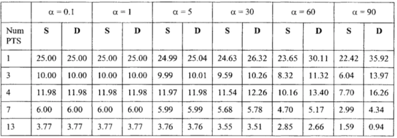
4.2a Quadrature test errors (percent) obtained for spherical TRI panel, with 0 0.1 degree and various o.

4.2b Quadrature test errors (percent) obtained for spherical TRI panel, with (X 0.1 degree and various 0.

Chapter

1

Introduction

Panel methods have been utilized extensively in aerodynamic and hydrodynamic design for several decades, beginning with the classic three-dimensional panel method developed by Hess and Smith in the 1960's [Hess 67]. This method was initially based on constant-strength sources and vortices on flat quadrilateral panels ('surface elements') distributed over the body; the adoption of these surface elements facilitated discretization of an arbitrary body sur-face and made it possible to analyze flows past realistically-shaped bodies. Since that time, a large number of variations on the original approach have been devised, although most can be classified as either velocity-field or field formulations [Lee 87]. The first potential-field formulation as adapted to the lifting-body problem is attributed to Morino, whose imple-mentation utilized a constant value of potential over each panel [Morino 74]. With the goal of increasing solution accuracy and computational performance, a number of so-called higher-order panel methods began to appear in the 1980's, e.g. [Hess 87]. However, many well-known codes still employ constant-strength panels (the latter sometimes being referred to as a low-order method); this reflects an on-going debate as to whether higher-order methods pose any real advantages over the low-order methods.

Generally speaking, a low-order method requires a substantially greater number of panels than that of a higher-order method, however, as the latter requires a greater number of degrees of freedom (unknowns) per panel, the overall size of the linear system of equations is not nec-essarily smaller for the higher-order method. This is one reason why comparing low-order and high-order panel methods is difficult at best.

Over the past decade researchers have addressed serious concerns as to the accuracy and convergence of low-order panel methods when applied to certain types of propeller blade

geometry, e.g., see [Hsin 91], [Pyo 94] and [Lee 99]. Such interest is indicative of further work to be done in this area.

In this thesis, a higher-order potential-based panel method utilizing Bezier basis functions is presented. The paper describes a method which incorporates variable-degree Bezier model-ing, not only for representation of the surface geometry, but also for the distribution of the velocity potential. The Bezier-based approach was inspired by a B-Spline higher-order method proposed by Lee and Kerwin [Lee 99] and still under development.

In modem computer-aided geometric design (CAGD), B-spline basis functions do in fact present a more powerful means of surface representation compared to Bezier surfaces, espe-cially for complex configurations like ship hulls. Today, B-spline-based NURBS surfaces are utilized as the de facto industry standard. On the other hand, a panel method, by definition, considers a discretization of the boundary into a collection of panels, and the complexity of each individual panel is far less than that of the surface as a whole. Individual panels can therefore be adequately represented using Bezier patches. Moreover, with respect to surface discretization, the Bezier formulation offers a distinct advantage over B-spline surfaces, in that Bezier patches can be rendered in both triangular and tensor-product (four-sided) forms.2 The availability of both types of patches gives the analyst more flexibility in choosing panel configurations, as for example, in the modeling of a hydrofoil or propeller tip. A sample dis-cretization of a hydrofoil is included herein to illustrate one possibility.

Some well-known panel codes in use today utilize panels that do not have conforming interfaces (e.g., neighboring panels connect at only one point along the edge). Using Bezier patches, it is a simple and straightforward matter to maintain full continuity of the surface along the entire perimeter of each panel, whether triangular, tensor-product or a combination of both types is used.

1. NURBS: Non-uniform rational B-splines

The present paper begins with a brief review of the fundamentals of potential-based panel methods. This is followed by a review of the fundamentals of Bezier curves, surfaces and functions in Chapter 3. Both triangular and tensor-product Bezier surfaces are addressed, as well as their role in representing scalar functions (potential distribution). The method for com-puting velocity via first-derivative computations of the Bezier surface and function is also

pre-sented.

The objective of this thesis is to develop a general-purpose variable-order method for application to non-lifting and lifting bodies in steady incompressible inviscid flow, including the important problem of predicting added mass.3 The method has been tested using a first-generation implementation coded in C++ using object-based technology. Computed results are compared with exact values for two applications: a) steady flow past a sphere and b) added mass of spheroid (ellipsoids of revolution). Very good agreement is demonstrated in both cases, as seen in Chapter 5.

A preliminary formulation for the lifting-body case is presented, however, further devel-opment and testing is required in order to ascertain the validity of the method for this problem domain. Various modeling issues and other considerations in the lifting-body problem are dis-cussed in some detail.

A panel-coupling technique referred to as velocity coupling is utilized to improve overall solution accuracy, and to eliminate or minimize the need for 'velocity-smoothing' or finite differencing operations on the potential during post processing. Whereas continuity of poten-tial is automatically guaranteed at panel interfaces, velocity coupling ensures continuity of velocity at prescribed nodes. The velocity-coupling technique introduces an alternate form of independent equation, applied in lieu of the boundary integral equation at appropriate loca-tions, and is found to be much faster to assemble in comparison to the integral equation.

3. The concept of added mass is usually associated with unsteady applications, however it is also a

valuable concept in certain steady-flow applications, e.g., the correction of the measured drag coeffi-cient in wind tunnels with diverging walls. In any case, the computation of the added mass itself is a steady problem.

Although the resulting matrix equation is hybrid in form, to date no solvability problems have been encountered through the use of this technique, when applied in the manner described in

Chapter 4.

Results of this initial investigation indicate that further development work on the Bezier-based panel method may be warranted, depending on the target application. Its applicability as an analysis tool for use ultimately in propeller blade design and analysis, for example, remains an open question, however there appear to be no technical limitations to preclude it from being developed toward that purpose. The Bezier-based method may be of utility in other

Chapter 2

Overview of Potential-Based Boundary

Integral Formulation

The boundary element or panel method is founded on Green's theorem, the well-known group of theorems that express equivalence between an integral over a domain in n dimensions to an integral over a domain in (n -1) dimensions.4 The boundary integral equation resulting from Green's theorem makes it possible to obtain solutions to three-dimensional boundary value problems via surface (boundary) discretization alone. For a large class of engineering prob-lems, the boundary integral equation relieves one from the arduous task of performing a dis-cretization of a volumetric domain, e.g., as in the finite element method. The comparative simplicity afforded by the boundary integral equation has long been a prime motivating factor driving the development of panel methods.

The starting point for the Bezier-based higher-order panel method described in Chapter 4 is a potential-based boundary integral equation, rather than a source-distribution integral equation. The latter was the basis of the original three-dimensional panel method developed by Hess and Smith in the early 1960's [Hess 64]; subsequently, a panel method using a poten-tial-field formulation was developed by Morino [Morino 74]. In principle, both methods yield identical solutions for the potential function, as discussed in [Sclavounos 87]. The potential-based method was selected for this thesis potential-based on considerations discussed in [Kerwin 87].5 Accordingly, this chapter will focus on the potential-based boundary integral formulation.

Before reviewing the boundary integral equation, the boundary-value problem for incom-pressible potential flow is discussed.

4. In general, Green theorems are equivalent to integration by parts. [Arfken 85] refers to Green's the-orem as a "corollary of Gauss's thethe-orem."

2.1

Boundary-value Problem for Incompressible Potential Flow

The primary task of the panel method described herein is the numerical computation of the unknown distribution of potential on the body boundary. Once the distribution of potential is computed, the potential-flow velocity and pressure fields may be determined. Before compu-tation of the potential can proceed, a boundary-value problem (BVP) must be defined in suit-able terms so that a corresponding matrix equation can be constructed and solved. Generally, the closer the match between the matrix equation and the BVP, the more reliable the solution, provided the BVP is well-posed to begin with.

The process of defining a BVP requires identification of the governing equations and boundary conditions characterizing the problem. The theory underlying potential-flow bound-ary-value problems is well known, e.g., see [Kellogg 29], [Lamb 32], [Hess 67], [Hess 72], [Morino 74], [Newman 77], [Hunt 80], [Moran 84], [Lee 87], [Kerwin 87], and [Hsin 90]. Accordingly, only a brief overview is provided here.

2.1.1

Potential Flow Governing Equations

The problem domain under consideration is the steady potential flow about a three-dimen-sional lifting or non-lifting body in an unbounded incompressible, inviscid fluid. The body is assumed to be rigid and held fixed with respect to an inertial coordinate system, and subject to an inflow velocity U0, as shown in Figure 2-1.

For analysis purposes a domain n = Q u 8Q is considered, where Q is an open simply-connected6 region with boundary aQ subdivided as

aQ = SB u SOu SW, (2.1)

where

SB is the body boundary.

So is a surface located far from the body and "surrounding" the body.

6. A 'simply-connected' region is one such that all circuits drawn within it are reducible. A circuit is

said is to be reducible if it is capable of being contracted to a point without passing out of the region. See [Lamb 32].

Sw is a branch surface connecting SB and S. Sw represents an infinitesimally thin trailing-vortex sheet shed from the trailing edge of a lifting body [Kerwin 87]. For non-lifting bodies, Sw can be regarded as a tube of infinitesimal radius, yield-ing no contribution to the boundary integral equation, e.g. see [Newman 77].

Soo n y n 00 X S W SWS UC SW n

Fig. 2.1 Schematic section of three-dimensional potential flow domain and boundary.

Strictly speaking, MQ does not actually enclose the body, i.e., the body itself is not contained within the domain.7 It should be noted that Sw is, conceptually speaking, a 'hollow cylinder'; the cross-section of this cylinder is distorted according to the manner in which the flow is

7. For explanatory purposes, and to help fix ideas, the domain boundary may be compared to the inside

surface of a large inflated balloon. At some location on the outer surface of the balloon a relatively tiny body is displaced toward the center of the balloon and held in place, without penetrating the bal-loon surface. The region of the balbal-loon in contact with the body becomes SB, and the remaining por-tion displaced inward becomes the branch surface Sw.

anticipated to detach from the tail end of the body. In the case of a lifting body (e.g., hydro-foil) with zero thickness at the trailing edge, S, has the outward appearance of a sheet, how-ever, is actually the hollow cylinder in a 'flattened state'. This configuration is necessary, not only to satisfy the requirement that the flow region be simply-connected, but also to facilitate a differential of potential between the upper and lower sides of the lifting body. Normal vec-tors to the boundary are defined as shown in Figure 2.1 (i.e., pointing toward the interior of the domain). In view of the foregoing discussion regarding Sw , it is normal practice to assign a normal vector to one side of Sw only, for the lifting-body problem. See Section 2.1.3.2 below.

Within Q, the flow is assumed to be irrotational, i.e., the vorticity co is zero:

o = VxV = 0 in Q. (2.2)

This assumption is based on certain premises. For the purpose of this thesis, the flow upstream of the body is assumed to be irrotational; then, according to Kelvin's theorem, a material vol-ume of fluid upstream of the body and initially irrotational will remain irrotational as the material volume moves over the body [Newman 77]. Lack of a no-slip condition at the body boundary and the assumption of an infinitesimally thin wake downstream of the body are abstract simplifications of the true viscous flow. Real viscous flows are characterized by the presence of boundary layers and viscous wakes; however, the slip-boundary and thin-wake assumptions present a reasonable approach for modeling of real non-separated flows over streamlined bodies.

The irrotationality assumption implies the existence of a unique scalar potential field, such that the velocity field V may be expressed as the gradient of a totalpotential (:

V = V . (2.3)

Alternatively, the velocity field may be expressed in terms of a perturbation potential $, whereby

V = U0 + V = UO + V# , (2.4)

and v is the disturbance velocity field corresponding to the perturbation potential. As pointed out in [Hess 67], utilization of the perturbation potential permits somewhat greater generaliza-tion in the types of flows to be considered, since the onset velocity field U, is not necessarily restricted to the class of irrotational flows.

Of the three conservation laws (mass, momentum and energy), only the first is needed in the formulation of the potential-flow boundary-value problem. With the restrictions stated herein, mass continuity is given by Laplace's equation, in terms of the potential (either form):

V2Q = 0 in Q (total potential) (2.5)

V20 = 0 in Q (perturbation potential) (2.6)

2.1.2 Kutta Condition

The lifting-body problem requires an auxiliary condition (Kutta condition) to ensure the

exist-ence of a finite velocity at the trailing edge. In its most general form the Kutta condition is

given as

V'1 < 00 at the trailing edge of the body. (2.7)

The same principle applies for the perturbation potential. The Kutta condition numerically constrains the potential in such a manner as to ensure a physically plausible flow field at the trailing edge, and the amount of circulation and lift generated by the body is restricted

accord-ingly.8

8. The relationship between circulation and lift is governed by the Kutta-Joukowski theorem. See, e.g.,

[Newman 77]. The circulation is defined as the line integral of the tangential component of the velocity along any closed curve (as may surround a hydrofoil):

2.1.3

Boundary Conditions

Typically, two types of boundary conditions are specified on 8Q, viz., Dirichlet and Neu-mann conditions. The former is synonymous with a known or specified potential and the latter refers to a known or specified normal gradient of the potential.9 _{The need for these boundary}

conditions becomes obvious when examining the boundary integral equation, discussed in Section 2.2. On a given region of OQ one is not ordinarily permitted to prescribe both a Dirichlet and a Neumann condition, however there are exceptions. In the usual case, both forms will be specified on their respective regions of the boundary, and no part of the bound-ary will lack one or the other.

The following sections address boundary conditions on SB, SW and So,, respectively.

2.1.3.1

Body Boundary

Typically, Dirichlet conditions are not specified on the body boundary, simply because the potential is unknown.10 Therefore, Neumann conditions must be specified on the body bound-ary. In the context of potential flow applications, a Neumann condition is equivalent to the kinematic boundary condition. Assuming the body is solid (i.e., no transpiration), the kine-matic boundary condition follows from the condition that the flow at the body boundary must be tangent to the body surface. For the total potential, the Neumann condition is

an

Using (2.4), the Neumann condition for the perturbation potential is

= n - V4= n -Uc on S. _(2.9)

an

9. The terms 'essential' and 'natural' are interchangeable with Dirichlet and Neumann, respectively. 10. This is the motivation behind the panel method in the first place!

2.1.3.2

Wake Boundary

Boundary conditions on the branch surface S, depend on whether the body is lifting or non-lifting. In the analysis of a non-lifting body, Sw is usually reduced to a tube of infinitesimal radius, as described in [Newman 77]. In this case, there is no contribution to the integral equa-tion from Sw; certainly, there is no surface upon which any boundary condiequa-tion could be pre-scribed. Although the 'utilization' of an infinitesimally small tube results in certain simplifications, it is not strictly required; other configurations of the 'wake' of a non-lifting body are conceivable.

Dirichlet conditions come into play in the analysis of a lifting body. The branch surface Sw is interpreted as a variable strength 'dipole sheet' equivalent to an idealization of the free trailing vortex system emanating from the trailing edge of the body.11 For convenience, S w denotes one-half of the wake boundary circumference (corresponding to either the 'upper' or 'lower' side), while Sw refers to the entire wake boundary circumference (or loosely speaking, both 'sides' of the wake sheet). Here, Sw is assigned to the 'upper' side of the lifting body, so that its normal vector is facing more or less in the positive y direction (see Fig. 2.1). For the pur-pose of this thesis, the position of the wake sheet is either known or assumed; regardless, the locations of all surfaces (i.e., the entire boundary MQ) are considered known and fixed, and a solution to the direct problem is sought (in contrast to the inverse problem, in which the posi-tion of a porposi-tion of the boundary is unknown and being sought, inevitably necessitating some kind of iterative procedure).

On the wake sheet, Dirichlet conditions cannot be specified explicitly, as the potential is unknown on Sw. However, the difference in potential at any point on Sw is expressible in terms of the potential at the trailing edge, as discussed in [Morino 74]. This 'implicit' Dirichlet condition is tied in with the Kutta condition, since the Kutta condition can be expressed in terms of the potentials on either side of the foil at the trailing edge. As the flow over the suction and pressure sides proceeds downstream from the leading edge stagnation

11. There is equivalence between the rate of change of the normal dipole strength along the surface, and

the strength of a vortex tangent to the surface (orientated perpendicularly to the dipole array). For further details, see [Hess 72].

point, the value of the potential changes, resulting in a more or less cumulative increase in the potential difference as the trailing edge is approached. This assumes the body is generating lift - the potential difference at the trailing edge is zero for a non-lifting body. As the wake of a foil is not able to sustain a pressure difference, no further change in the potential difference occurs as the flow leaves the trailing edge. Whatever potential difference has accrued at the

trailing edge is all there will be, and the difference is maintained as the flow proceeds away from the body.

Further aspects of the wake boundary and Kutta condition are discussed in Section 2.2 and Chapter 4.

2.1.3.3

Far Boundary

Treatment of the far boundary S, depends on whether the total or perturbation potential is utilized. This is one region in which both Dirichlet and Neumann conditions apply, and since both the potential and the normal gradient are known on S., the corresponding surface inte-gral in the boundary inteinte-gral equation can be computed and reduced to a simple quantity. As the perturbation potential is easier to deal with, it is discussed first.

On the far boundary S., both the perturbation potential and the normal gradient of the poten-tial are expected to vanish in the limit as the distance between the surface and body approaches infinity:

#

and

V# -+ 0, at infinity. (2.11)

Considering this hypothetical boundary for S., there is no contribution to the integral equa-tion and consequently no further consideraequa-tion is required with respect to boundary condiequa-tions

For the total potential, matters are somewhat more complicated, but reconcilable. Neither the total potential nor the normal gradient (i.e., the velocity) vanish everywhere on S,. How-ever, these quantities are known, provided the geometry of S, is specified and the distance between the body and S. is sufficiently large so that any disturbance due to the presence of the body may be regarded as negligible, i.e.,

(D -+ D,, at infinity, (2.12)

and

VP -> U,, at infinity. (2.13)

It turns out that the corresponding surface integral in the integral equation evaluates to a sim-ple quantity proportional to the incident potential ,,.12 Using the resulting simplified form of the boundary integral equation for the total potential, again, no further consideration is required with respect to boundary conditions at the far boundary.

2.2 Boundary Integral Equation

The boundary integral equation is the backbone of the panel method. As pointed out by [Rob-ertson 65], the significance of integral equations is the equivalence theorem, which states:

The solution of an integral equation is a solution of the corresponding boundary-value problem and vice versa.13

By casting the governing equation (2.5) or (2.6) into an boundary integral equation, a solution

can be obtained by considering what is happening on the boundary OQ alone, while disre-garding details within the domain Q itself. The overall simplification and resulting economy

12. It can be shown that for a sphere surrounding the body, the Dirichlet condition contributes two-thirds toward (D., , while the Neumann condition contributes the remaining one-third. The Dirichlet and Neumann conditions are associated with the dipole and source terms, respectively, in Green's

for-mula.

13. This, according to [Robertson 65], is demonstrated in Courant and Hilbert (Methods of Mathematical

of effort achieved with the integral equation is significant in comparison to the original boundary value problem (differential equation).

From the standpoint of implementing a panel code, the main purpose of the boundary inte-gral equation is to provide a means for generating a system of linear algebraic equations to be solved in order to yield the distribution of potential on the body boundary.

In this section, only the potential-based boundary integral equation is addressed. For dis-cussion purposes, it is useful to distinguish between the basic integral equation and the

bound-ary integral equation. The basic integral equation is a Fredholm equation of the second kind 4

giving the potential at a point anywhere within the domain Q, in terms of the potential and its normal derivatives on the boundary. The basic integral equation suffers from the fact that it becomes strongly singular1 5 _{if the field point (i.e., the point at which the unknown potential is} sought) lies on the boundary. Nonetheless, the basic integral equation is important in two respects:

1. The boundary integral equation is derived from the basic integral equation;

2. The basic integral equation can be used to compute the potential away from the bound-ary after the boundbound-ary solution is obtained.

The 'boundary integral equation' refers to an integral equation of the second kind in which the potential is expressed entirely in terms of values on the boundary 8M. The boundary inte-gral equation is essentially 'de-singularized', as the kernel does not, strictly speaking, become infinite at any point in the range of integration. De-singularization is accomplished by inte-grating over an infinitesimal region S. surrounding the field point, yielding a free value of potential which is simply added to the original term located outside the integral. This process subsequently alters the range of integration, since the integral has already been evaluated over S.. Therefore S. must be excluded, in a manner analogous to the Cauchy principal integral.16

14. A Fredholm integral equation is a linear integral equation in which the limits of integration are fixed. An integral equation of the second kind is one in which the unknown function appears both inside and outside the integral(s). For more details, see, e.g., [Arfken 85].

15. There are two types of kernels encountered in this application. Both types are strongly singular as

they contain a difference term (x -4)' in the denominator, with cx 1 and ox = 2, respectively. The former is referred to a Cauchy singularity. See, e.g., [Jerri 99].

The basic integral equation can be deduced in several ways. The traditional approach employs the symmetrical form of Green's theorem. A modem approach uses the concept of distribu-tion, which according to [Brebbia 89], "illustrates the degree of continuity required of the functions and the importance of the accurate treatment of the boundary conditions."

No derivations of the basic integral equation or boundary integral equation are provided herein - various derivations are given in [Newman 77], [Kerwin 87], [Brebbia 89], and [Chari 00]. The basic integral equation is presented in the next section, followed by the boundary integral equations in terms of the total potential and perturbation potential, respectively.

2.2.1 Basic Integral Equation

The basic integral equation, better known as Green's formula or Green's third identity, is given as

(x) (x; ( ()G(x; )]d. (2.14)

ffan,

an(.4

This equation gives the potential at a field point x in terms of the potential and normal gradi-ent distribution on the boundary MQ, where integration is performed with respect to the dummy variable 4. The quantity G(x; 4) is defined as

G(x; 4) = - 1 (2.15)

47rlx-41

where (x - )f is the distance between position vectors x = (x, y, z) and 4

(,

).

Although best known as Green's function, G(x; ) is sometimes called thefundamental

solu-16. Cauchy's principal value of an integral of a functionf(x) that becomes infinite at an interior point

x = x, of the interval of integration (a, b) is the limit

SX0 - 6 b

lim f(x)dx +

J

w X + /

tion, e.g., as in [Brebbia 89], since it is the simplest possible non-trivial solution to the

poten-tial-flow governing equation, i.e., (2.5) or (2.6). More specifically, it represents the potential at the field point induced by a unit source at , and for this reason G(x; ) is also referred to as the Rankine singularity. As such, (2.11) satisfies Laplace's equation everywhere except at the source point 4, so that the fundamental solution can be expressed as

V2G(x; ) = 6(x; ), (2.16)

where 6(x; 4) is the delta function, i.e.,

6(x; )for x (2.17)

00 _{for x}

The delta function has the peculiar but powerful property

J

which extends to distributions of functions, so that for a distribution of potential

f (x; 4)d = (1(x). (2.19)

Q

Referring to the second integral in (2.14), the normal gradient of Green's function represents another type of singularity, viz, a dipole, which is derivable from the fundamental singularity (source). Whereas a source exhibits no directivity, a dipole has an orientation corresponding to a line on which a source and sink (negative source) approach one another in the limit as the gap approaches zero and the strength of each singularity approaches infinity. By convention, the positive direction is in the direction of the positive source. The normal gradient of Green's

aG(x; ) _ (x - n(3) 4) unit-strength dipole directed along n . (2.20)

an

4ix-I

2.2.2 Boundary Integral Equation

The boundary integral equation is obtained from the basic integral equation by locating the field point on the boundary and evaluating the surface integral in way of the field point by considering an infinitesimally small region S, surrounding the field point. This process is

effectively a 'de-singularization' of the basic integral equation. The boundary integral

equa-tion based on (2.14) is

T Q(x)

f

I

iG(x;

M aQE,

The coefficient T is the solid angle (in steradians) subtended at the field point on the bound-ary, divided by 47r. See, e.g., [Hunt 80]. The usual value for T is 1/2, corresponding to a

smooth continuous surface where the field point is situated. T may vary between 0 and 1, depending on the geometrical configuration of the body boundary and wake surface.

2.2.2.1

Total Potential Formulation

By taking boundary conditions into account as discussed in Section 2.1.3, the resulting

bound-ary integral equation for the lifting-body problem is given as

T1(x) = ty(x) - q ()G x - f f A (4T1)Gx(X )d , (2.22)

SB-S,

where At((TE) is the difference in potential 'across' the trailing edge (i.e., from one side of

the wake sheet to the other), with the dummy variable 4 being associated with a position on

the trailing edge, TE, corresponding to the location at which the flow departed the trailing edge.

For the non-lifting problem, the second integral in (2.22) is omitted.

2.2.2.2

Perturbation Potential Formulation

Taking boundary conditions into account as discussed in Section 2.1.3 for the perturbation potential, the resulting boundary integral equation for the lifting-body problem is given as

T4(x) = G(x; )) a n,

Sa - Se

- JJO( )Gan x - - fJA$(4TE)G x )d'

S3 - d) _{S W}

where the meaning of AD( TE) is described in Section 2.2.2.1 above.

For the non-lifting problem, the last integral in (2.23) is omitted.

Chapter 3

Fundamentals of Bezier Curves, Surfaces and Functions

3.1 Historical Background

The development of Bezier curves is attributed to P. de Casteljau and P. Bezier, whose efforts were carried out independently on behalf of Citroen (beginning in 1959) and Renault (begin-ning in 1962), respectively.1 8 The introduction of Bezier curves presented an alternative approach to cubic spline techniques developed by J. Ferguson at Boeing in the 1950's.

Only later was it discovered that the curves named after Bezier were intimately connected with the classical Bernstein polynomials; in 1970, R. Forrest discovered that the Bernstein polynomials were indeed the basis functions for Bezier curves. Meanwhile, efforts by de Boor at General Motors led to a practical utilization of B-splines (basis splines); although B-splines were actually investigated by I. Schoenberg during World War II, many years passed before an accurate and stable means of computing with B-splines became available. A short time after de Boor's landmark paper, "On calculating with B-splines," appeared in 1972, Gordon and Riesenfeld demonstrated that Bezier curves were a special case of B-spline curves, paving the way for a more unified treatment of the various methods developed on both sides of the Atlantic.

18.According to [Farm 99], 1959 marks the birth of computer-aided geometric design (CAGD), when Citroen hired P. de Casteljau to develop mathematical tools to more fully exploit the capabilities of their numerically-controlled milling machines. De Casteljau invented what he called Courbes a

Poles, what are now known, ironically, as Bezier curves. P. Bezier learned about Citroen's 'very

secretive' efforts and was able to develop a functional CAGD system himself at Renault; his firm allowed him to widely publicize the method.

In this thesis, only the Bezier formulation is considered. The next section begins with a brief description of the Bernstein polynomials. Subsequent sections treat Bezier curves, func-tions and surfaces.

3.2

Bernstein Polynomials

Bernstein polynomials are the key component in the Bezier representation of curves, surfaces

and functions. Bernstein polynomials of degree n are defined as follows:

Br -( -t)l r, r = 0(1)n . (3.1)

The parameter t takes on values anywhere in the closed interval between 0 and 1, i.e.,

t e [0, 1]. An nth-degree Bernstein polynomial comprises a family of (n + 1) polynomial

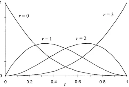
curves spanning the closed interval [0, 1]. All the polynomials are non-negative on this inter-val. At the end points the values of all the polynomials are zero, except for the first and last polynomials, B n and B'1 _{, respectively; the former is equal to 1 at the beginning of the} parameter interval (t = 0) and the latter is equal to 1 at the end of the interval (t = 1).19

The cubic Bernstein polynomials B3 _{, for example, take the shape seen in Figure 3.1, for}

t e [0, 1].

The Bernstein polynomials form a so-called partition of unity, an important property such that the sum of all polynomials is equal to unity for any given value of t in the parameter interval [0, 1], i.e.,

ti

B,.n (t) = 1. (3.2)

r 0

19. Interestingly, a Bernstein polynomial curve is identical to a binomial probability distribution of a

random variable, where t is the probability of getting r successes in n trials. Compare (3.1) with the probability distribution formula given, e.g., in [Freund 80].

1

r =0 r= 3

r r 2

0 f

0 0.2 0.4 t 0.6 0.8 1

Fig. 3.1 Bernstein polynomials of degree 3.

3.3 Bezier Curves and Functions

A Bezier curve can be defined using the Bernstein polynomials as basis functions. A Bezier

curve of degree n in parametric form is defined as

II

X(t) b B" (t), (3.3)

i= 0

with coefficients by e 9 d, d = 1, 2, 3. When bi are chosen as vectors in 12 or 93 3they are referred to as Bezier controlpoints or simply Bezier points. If the coefficients bi are scalar val-ues, they are called Bezier ordinates. The set of straight lines connecting the Bezier points is called the Bezier polygon, as shown in Figure 3.2.

The Bezier curve (3.3) is independent of the coordinate system, due to the partition-of-unity property (3.2). If this property did not hold, then a simple translation, rotation or scaling would destroy the relationship between X (the curve) and b (the Bezier control points).

If the Bezier ordinates bi are located at parameter values t = i/n, then the parametric for-mula (3.3) for a Bezier curve reduces to a Bezierfunction. See Figure 3.3.

b2 _b3

b, _b4

bo

Fig. 3.2 A Bezier curve of degree 4 and its associated Bezier polygon.

b2

b,

bo

0 1/3 2/3 1 t

The k-th derivative of a Bezier curve is given by n-k xk) (n k _{I A} i=0 n-k (3.4)

where Ak are forward difference operators defined as

Ab, ab h+ - by ,

2

A b1 = A(A b)= A(b1j 1 , bi) = bi+ 2 - 2b jI + bi,

k Ak b.

Z

Important properties of Bezier curves are listed below:

- The Bezier curve begins and ends at bo and bn, respectively.

- The edges bo b1 and bn- 1 bn of the Bezier polygon are tangent to the curve.

" The k-th derivative at the endpoint of a Bezier curve depends only on the boundary point and its k neighbors.

3.3 Bezier Surfaces and Related Functions

Bezier expansions can be formulated for two types of surface patches:

- tensor-product (four-sided) - triangular

3.3.1

Tensor-product Bezier Surfaces and Functions

The surface geometry of a tensor-product Bezier patch is represented by the following rela-tion:

X(u,v) = b g B"(u) Bkm(v) (3.8)

i=0 k=O

where bik are Bezier points distributed in three dimensional space and u, v e [0, 1]. The Bez-ier points bik comprise a three-dimensional BezBez-ier net controlling the geometry of the patch. The Bezier net is analogous to the Bezier polygonal associated with Bezier curves. If the Bez-ier points are scalar-valued, then (3.8) is a function defined over the planar simplex, on which

u, v e [0, 1], and a scalar distribution analogous to that shown for Bezier curves exists (see

Fig. 3.3). In this case, the control points are referred to as Bezier ordinates (as for the Bezier curve).

The total number of Bezier control points bik associated with a single QUAD panel is (np + 1)(m + 1).

The partial derivatives of a tensor-product Bezier surfaces are given by:

r 8 n-r__ rO n-r

X(u, v) = A bik B, (u) Bk (v) , (3.9)

O u i=O k=O

s_ X_,_)_m m' s b Bu)B (),3.)

d v _=0 k=O

where the forward differences are given by

For derivatives of a function, X and b in (3.9) to (3.11) are replaced by their scalar equiva-lents. Refer to [Hoschek 93] for further details.

3.3.2 Triangular Bezier Surfaces and Functions

A triangular Bezier surface is defined by the following parametric representation:

X(u) = b B1_{(u), (3.12)}

where B n(u) are the generalized Bernstein polynomials of degree n defined as

B n(u) _I = B ( = . u ! V /' , (3.13)

Uk (U) !j! k!

and b, are control points (in 2-D or 3-D) that collectively form a Bezier net. In (3.12) and (3.13), I is defined as (i,j, k)T , with i,j, and k subject to the constraint i +j + k = n, with i,j, and k non-negative; u is shorthand for (u, v, w)T , the three barycentric coordinates with respect to a base triangle (planar), as shown in Fig. 3.4. For any point on the base triangle, the bary-centric coordinates always sum to unity: u + v + w 1, and the coordinates are non-negative.

V

W=O

W

U

The vertices of the triangle are represented by upper-case U, V, and W, corresponding to u 1, v = 1 and w = 1, respectively, so that any point on the planar triangle can be expressed as

P(u, v, w) = uU + vV + wW. (3.14)

The barycentric coordinates are invariant under linear (affine) transformations. This prop-erty allows one to consider different shapes of the base triangle without affecting the Bezier patch itself.

The sum in (3.12) involves a total of (n + 1)(n + 2)/2 terms. For example, a triangular panel of degree 3 comprises 10 terms, yielding a three-dimensional Bezier net consisting of 10 Bezier points. For this case, the control point subscripts ij, k are identified with the base tri-angle as shown in Fig. 3.5. Control points associated with the corner points of the base trian-gle are located on the actual vertices of the Bezier triangular patch.

b03O V b021 _b120 bol 2 _b~l bl0 0 W U b003 b102 b_{20 1} b₃₀₀

If the control points in (3.12) are scalar-valued, the control points are referred to as Bezier ordinates (just as in the case of a Bezier curve). In this case, the Bezier 'surface' is a function defined over the base triangle, and the situation is analogous to that shown in Fig. 3.3 for the curve.

Derivatives on triangular Bezier patches cannot be expressed as partial derivatives, due to the constraint u + v + w = 1. However, derivatives can be expressed with respect to one of the parameters with the condition that one of the other parameters is held constant, e.g., see

[Hoschek 93]: DX duv _{= constant} DX du w= constant DXu dv n i +j+ k=n -I =n i+j +k=n-(bij A - bjk ) B I _B11v B)1_{k (u, V, w)} = n I =constant i +j + k =n -1

For derivatives of a function, X and b in (3.15) to (3.17) are replaced by their scalar equiva-lents. (bb ) (U, V, W) ( b jk - b ) B k ),I (3.15) (3.16) (3.17)

Chapter 4

Bezier Based Higher Order Panel Method

This chapter presents the main elements of the Bezier-based higher-order panel method. The development of this method builds largely on previous chapters covering fundamentals of the boundary integral equation and Bezier representation of surfaces and functions.

4.1 Body and Wake Surface Discretization

Application of the method begins with a boundary mesh-generation process, whereby the sur-face of the body is decomposed into a set of unique, non-overlapping Bezier patches or

pan-els. The collection of panels may comprise a combination of tensor-product Bezier surfaces

and triangular Bezier surfaces, referred to here as QUAD and TRI panels, respectively. The wake boundary, when modeled explicitly, is partitioned in a similar manner (except that, as discussed in Chapter 2, only one side of an infinitesimally thin wake sheet is modeled).20

A general requirement is that the interface between neighboring panels be continuous, i.e.,

CD continuity should exist at each such interface. Any gaps or 'leakage' between adjoining panels would likely have an adverse effect on the solution and therefore should be avoided. CD continuity is guaranteed by ensuring that adjoining panels share the same Bezier thread along the common edge, i.e., the Bezier points on that edge are common to both panels; this is true whether the interface between the two panels is QUAD-QUAD, TRI-TRI or QUAD-TR.

k

The body boundary SB is discretized into a total of NB individual panels AB such that

NB _k

SB AB U AB , (4.1)

k = I

20. As discussed in Chapter 2, typically the wake boundary for non-lifting bodies is practically nonexist-ent. For a lifting body, the geometry of the wake sheet is given or assumed.

where the over-bar denotes closure (i.e., A = A + aA). Similarly, an explicit wake boundary

k

Sw is discretized into a total of Nw individual panels A, satisfying

Nw

k

SW = Aw= U Aw . _(4.2)

k = 1

Conceptually, Sw is typically regarded as being semi-infinite in extent, however, as a practical matter, the number of panels in the wake is necessarily restricted to a finite quantity, as indi-cated in (4.2).21

The trailing edge of the body is defined as a closed curve formed by the intersection of the body and wake boundaries:

CTE =BTr- w. (4.3)

In a typical analysis of a lifting body, the trailing edge thickness is considered to be zero, in which case the area enclosed by CTE approaches zero and the trailing edge resembles an open line or non-closed curve; despite any such appearance, however, the trailing edge must be treated as a closed curve if the body is to generate lift, as discussed in Chapter 2.

CI continuity between panels is ensured when the panels connect in a 'simple',

conform-ing manner, so that

A r-n A an entire edge or an entire vertex of each panel .22 (44)

21. There are a number of ways in which this apparent dilemma is treated. For example, a semi-infinite line vortex can be used to emulate a 'rolled-up' wake sheet, as the potential induced by such a line vortex is known in closed form. For the propeller problem, see discussion in [Kerwin 78]. Details of the various approaches are beyond the scope of this thesis. One approach is simply to model the wake as a finite length sheet and rely on the fact that the influence of a normal dipole diminishes rap-idly with distance from the body, on account of two effects. The potential induced at a field point on the body is 1) inversely proportional to the square of the distance between the field point and the point on the wake boundary, and 2) proportional to the dot product between the unit normal vector on the wake and the unit vector collinear with the field and wake points. The former obviously indi-cates a strong attenuating effect, and the latter tends to a low value for any field point on the blade, with increasing distance.

As mentioned, this condition is not difficult to achieve.

4.2

Bezier Modeling of Surface Geometry

The surface geometry of a QUAD panel is represented by the following tensor-product rela-tion:

n ni

nn

X(u,v) = b 1B,"(u) B"(v) . (4.5)

i=Oj=O

Typically, the degree of the Bezier polynomial corresponding to the parameter u is the same as that associated with the parameter v, in which case n = m; however, this is not a require-ment. There may be panel configurations in which it is appropriate for n to differ from m.

A TRI-panel surface is defined by the following parametric representation:

X(u) = b, Bi"u (4.6)

Ill = n

As discussed in the previous chapter, the above sum involves a total of (n + 1)(n+ 2)/2 terms;

for instance, a TRI panel of degree 3 comprises 10 terms, yielding a Bezier net consisting of

10 Bezier points. Also, u is shorthand for (u, v, w), the three barycentric coordinates, the sum

of which is always unity: u + V + w = 1.

4.3

Bezier Modeling of Potential Distribution

The velocity potential distribution on a panel is modeled by means of a scalar Bezier function. The velocity potential over the entire body boundary is modeled using a collection of scalar Bezier patches. A one-to-one correspondence exists between the set of geometrical patches

and the set of functional patches, so that each and every panel is characterized by a pair of

On any given panel, the scalar Bezier function is expressed in terms of a distribution of local potential ordinates

{

D(u, v) = II B (u) B m(v) ,(4.7)

i=0 j=0

where degree n and degree m correspond to the u-wise and v-wise coordinate parameters,

respectively. While n and m are analogous to n and m of the Bezier surface, there is no requirement that they be equal. Indeed, the Bezier potential patch and the Bezier surface patch are independent in this respect. The scalar Bezier ordinates T i, comprise a Bezier net control-ling the distribution of the potential over the QUAD panel and are analogous to the vector-val-ued Bezier points bgy which control the panel surface geometry. The total number of unknown potential ordinates (p associated with a single QUAD panel is L = (n + 1)(m + 1); each potential ordinate is associated with a local panel node i, yielding a total of L such nodes on the panel. The local panel nodes { x } are three-dimensional position vectors corresponding to a uniform distribution of the panel coordinates (u, v), where u e [0, 1], v e [0, 1], so that on any given panel, the nodes are unique, i.e., ix x for i #j

On TRI panels, the potential is given as

t(u) = 2 p1 B"(u) , (4.8)

Il = 124

where B2n(u) are the generalized Bernstein polynomials of degree n . Again, n is analogous to n, but there is no requirement that they be equal, and as with the QUAD panel, the triangu-lar Bezier potential patch is independent from its Bezier surface patch, insofar as difference in degree is concerned. The scalar Bezier ordinates 9 comprise a Bezier net controlling the dis-tribution of the potential over the TRI panel and are analogous to the vector-valued Bezier

points b, which control the panel surface geometry. The total number of unknown potential