Arctic Ocean circulation in an idealized numerical model

Arctic Ocean circulation in an idealized numerical

MASSACHUSETTS INST E OF TECHNOLOGY

OCT 2 12008

LIBRARIES

model

by

Peter Joseph Sugimura

Submitted in partial fulfillment of the requirements for the degree of

Master of Science

at the

MASSACHUSETTS INSTITUTE OF TECHNOLOGY

and the

WOODS HOLE OCEANOGRAPHIC INSTITUTION

September 2008

@Peter

J. Sugimura, 2008. All rights reserved.

The author hereby grants to MIT and WHOI permission to reproduce

and distribute publicly paper and electronic copies of this thesis

document in whole or in part.

A uthor ...

...

MIT/WHOI joint program in Physical Oceanography

July 18, 2008

C ertified by .... ,, ... V ... ...

Peter Winsor

Assistant Scientist

Thesis Supervisor

Accepted by.

Raffaele Ferrari

Associate Professor

Chairman, Joint Committee for Physical Oceanography

Arctic Ocean circulation in an idealized numerical model

by

Peter Joseph Sugimura

Submitted to the MIT/WHOI Joint Program in Physical Oceanography on July 18, 2008, in partial fulfillment of the requirements for

the degree of Master of Science

Abstract

The mid-to-deep Arctic Ocean is generally characterized by a cyclonic circulation, contained along shelves and ridges. Here we analyze the general Arctic circulation using an idealized numerical model consisting of a circular basin with two channels acting as inflow and outflow. We analyze the circulation (direction, strength and sensitivity) for wind forcing with and without bathymetry (ridges), and with and without stratification. We find that the circulation is modified drastically by both bathymetry and wind direction, where an altered wind field can change both the direction of the horizontal basin circulation as well as the strength of the inflow and outflow. The idealized circulations imply that the Arctic circulation, and the associated export of freshwater, can easily switch states in a changing climate.

Thesis Supervisor:

Peter Winsor Assistant Scientist

Acknowledgments

I would not have completed this thesis without the support of many. Foremost is my advisor, Peter Winsor, whose ideas, support, and his enthusiasm were an invaluable help. Jean-Michel was a great help both during and after my learning process in running MITgcm. Without his help and suggestions, my model might never have

gotten off the ground. Many thanks go to my fellow physical oceanographers - Jinbo,

Evgeny, and Christy. We started as classmates, but grew to become friends. My experience would also not be complete without the friendships of fellow graduate students at both MIT and WHOI. And I never would have even made to where I am without the loving support of my parents. Finally, a special thanks go to Julie for her support and encouragement of during throughout my time in the Joint Program.

Contents

1 Introduction 13

2 The Current Understanding of the Arctic 17

3 Forcing from Potential Vorticity Advection 21

4 Arctic Circulation in an Idealized Numerical Model 27

4.1 Introduction ... ... .. 27

4.2 Model Description ... ... 30

4.3 Results ... ... .. 32

4.3.1 Wind Forcing ... ... 32

4.3.2 Addition of Bathymetry (Ridges) . ... 37

4.3.3 Effect of Stratification ... ... 39

4.4 Discussion and Conclusions ... .... 42

5 Conclusion 47

List of Figures

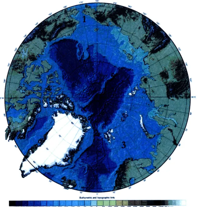
1-1 Map of the Arctic with bathymetry from the International Bathymetric Chart of the Arctic Ocean (IBCAO). 1) Bering Strait 2) Fram Strait

3) Barents Sea 4) Canadian Archipelago 5) Lomonosov Ridge . . . . 15

2-1 Typical temperature, salinity, and density profiles in the Arctic Ocean.

From Aagaard and Coachman, 1975 [1] . ... 19

3-1 PV forcing in a symmetric basin: a) SSH b) depth contours .... . 22

3-2 PV forcing in for a) a symmetric basin b) high PV outflow c) depth contours for symmetric basin d) depth contours for asymmetric basin

(tilted so that right is shallower, left is deeper). . ... 25

4-1 Wind forcing on a closed basin a) SSH b) Velocity vectors of the flow

in the basin . . . 34

4-2 SSH for an open basin with a) along channel wind b) cross channel wind 35 4-3 Annular wind forcing in an open basin a) SSH for cyclonic wind b)

SSH for anticyclonic wind c) velocity for cyclonic wind d) velocity for

anticylonic wind ... ... .. ... .. 36

4-4 Wind forcing in an open basin with ridges. SSH for: a) along channel wind and cross channel ridge b) cross channel wind and cross channel ridge c) along channel wind and along channel ridge d) cross channel

4-5 Along channel wind forcing in an open basin comparing the effects of ridges and stratification. SSH for a) Control run (unstratified, no ridge) b) Unstratified with a shallow ridge c) Unstratified with a deep

ridge d) Stratified with a shallow ridge . ... 41

4-6 Mean SLP in the Arctic for July and August from 1993-1996. Data

taken from NCEP/NCAR reanalysis project. . ... . 45

4-7 f/H contours in and open basin with a) no ridges b) shallow ridge . . 46

A-1 Anticyclonic wind forcing for a basin with a) normal magnitude winds

b) strong magnitude winds (3x normal) ... .... ... 49

A-2 Cyclonic wind with a shallow ridge parallel to the channels: a) SSH b)

depth contours ... . . .. . ... 50

A-3 Wind forcing parallel to the channels in an open basin with a) normal

strength winds b) strong winds (3x normal) . ... 51

A-4 Wind forcing parallel to the channels in an open basin with ridges of varying orientation: a) shallow ridge parallel to channels b) deep ridge parallel to channels c) shallow ridge perpendicular to channels d) deep

ridge perpendicular to channels ... .. 52

A-5 Wind forcing perpendicular to channels in an open basin with varying ridge orientations: a) shallow ridge parallel to channels b) deep ridge parallel to channels c) shallow ridge perpendicular to channels d) deep

ridge perpendicular to channels . ... .. 53

A-6 Zonal wind forcing in a closed basin: a) homogeneous b) stratified . . 54

A-7 Wind forcing parallel to channels in a stratified basin: a) normal winds b) strong winds (3x normal) c) normal winds with a ridge parallel to

List of Tables

4.1 Parallel and Perpendicular refer to the orientation of wind/ridges rel-ative to the channel. For wind orientation, "Strong" means 3 times the strength of normal forcing. For ridge orientation, "Deep" refers to a deep ridge at depth of 860m, if unspecified, the ridge is equal to the

Chapter 1

Introduction

Oceanography is a young science; Arctic oceanography younger still. The methods and instruments that have been honed in the sub-polar and tropical oceans have rarely been applied to the Arctic Ocean: not because the Arctic is dull or lacks importance, but because of the harsh conditions of the Arctic. Beyond the usual oceanography challenges of working in a salty environment that can play havoc with electronics, a thick ice pack necessitates use of slow icebreakers and icebergs threaten instruments that dare sample the upper water column. The end result is a relative lack of knowl-edge in a region thought to be highly sensitive to global climate change.

The climate system of the Arctic Ocean is controlled via intricate feedbacks be-tween the atmosphere, sea ice, and the ocean. These feedbacks act on daily, seasonal, annual, and decadal time scales and on spatial scales from meters to hundreds of kilometers. The processes which act at smaller scales are easier to study, given the lack of long-term measurements and scattered observations, but the actual processes by which sea ice, the atmosphere, and the ocean interact on time scales longer than annual time scales are a, current topic of investigation. The enormity of the task facing polar scientists has been recognized by the creation of the International Polar Year (IPY) 2007-2009. During IPY, an international research effort will converge on the poles to study aspects of polar science ranging from physics to biology to

an-thropology - and everything in-between. A planning group has set forth a series of questions and themes in an attempt to focus research efforts. The first question of the first theme is revealing:

What are the _{current composition and the patterns of circulation of the} high latitude ocean-atmosphere-ice system; and what are the interactive processes that drive high-latitude circulation? - A framework for the In-ternational Polar Year 2007-2008 [3]

It is sobering to acknowledge that the current composition and the patterns of circulation of the Arctic Ocean circulation are still a valid research subject; that the frontier of knowledge has barely advanced since the first Arctic oceanographers such as Nansen first explored the Arctic. At the same time, it is exciting to imagine that while many fundamental discoveries have been made in the past, many more are yet to be made; some which may have relevance towards the pressing issue of global climate change.

This thesis will examine the effect of variable wind forcing on the Arctic circulation in an idealized Arctic numerical model. The attached paper describes how varying an idealized wind field can drastically affect the circulation. It is also shown that shifts in the historical wind field analogous to the modeled idealized wind fields have recently been observed. In order to give context to the results, the basic state of Arctic Ocean circulation will first be described. Next, the motivation for this problem will be discussed. After the aforementioned paper, a few caveats to the approach will be discussed, as will suggestions for future directions this work may take.

9O

Bathyrmetrc and topograpihi t~h

-5000-4000-3oo -250.-2oo-ISOO1-1000 -00 -200 -100 -50 -25 -10 0 50 100 200 300 400 500 600 700 00 1000 W hrs)

Figure 1-1: Map of the Arctic with bathymetry from the International Bathymetric Chart of the Arctic Ocean (IBCAO). 1) Bering Strait 2) Fram Strait 3) Barents Sea 4) Canadian Archipelago 5) Lomonosov Ridge

Chapter 2

The Current Understanding of the

Arctic

The geography of the Arctic Ocean is often contrasted to the Southern Ocean. The Southern Ocean is bounded by land on its polar side, but has broad connections to the surrounding Pacific, Atlantic, and Indian Oceans. The Arctic Ocean on the other hand, is a mediterranean sea, constrained by land except for a few connections which connect to the Atlantic and Pacific Oceans. These straits are the narrow and shallow Bering Strait, the narrow but deep Fram Strait, the broad and shallow Barents Sea, and the small but numerous pathways that make up the Canadian Archipelago (Figure

1-1).

In addition to being a mediterranean sea, the Arctic has many other interesting properties. It has an area of 9.5 x 106 km2 - roughly the area of the United States. Ice covers an area of approximately 7.8 x 106 km2 in September and 14.8 x 106 km2 in March [2]. Many reasons conspire to ensure that the ice cap lasts the summer (for the near future anyways). The air temperature averages below -30' C in the winter and near freezing during summer. In addition, the tilt of the Earth's axis ensures that no light reaches the Arctic during the winter. Also, the high albedo of snow and ice limits the radiation absorbed and delays spring melt. Finally, although the Arctic

occupies 1.5% of the world's ocean surface area, it receives 10% of the river runoff. This large amount of fresh water flux caps the surface of the Arctic with a layer of relatively fresh water which allows the water in the shallow mixed layer to cool to the freezing point.

One third of the Arctic is composed of shallow Eurasian seas less than 200 meters in depth. It is these shallow seas where new ice is usually formed when wind pushes old ice offshore to expose surface water to freezing conditions. In the interior, two large basins, the Canadian and Eurasian, both reach depths of over 4000 meters. They are separated by the Lomnonosov Ridge that transects the Arctic from Greenland to Russia, passing near the North Pole.

Shelves and ridges are important because bathymetry is thought to have a large impact on the Arctic circulation. At the shelf break, a rim current travels around the Arctic in a cyclonic direction. At the ridges which transect the interior Arctic, relatively large currents (compared to the basin interiors) have been inferred from the measurements. The deep basins are quiet and sheltered because of minimal of deep convection in the Arctic (aside from a small amount of dense water production from polynyas). The Canada Basin is isolated enough so that geothermal heating from the ocean bottom is an important factor for deep mixing [14].

Water masses entering the Arctic from the Pacific and Atlantic have distinct salinity, temperature, and oxygen levels which can be measured to track its progress throughout the Arctic. The surface waters of the Arctic are relatively cold (below 0O C) and fresh (30-32 psu) compared to Atlantic water (salinity of 35 psu, temperature greater than 00 C). The water entering from the Atlantic salty enough so that upon entering the Arctic, the warm water mass counter-intuitively sinks below the cold, fresh surface layer of the Arctic. The end result is an easily tracked warm maximum from about 200m to 800m which is called the Atlantic layer. After entering the Arctic through the Fram Strait (west of Svalbard) and Barents Sea, the Atlantic layer travels cyclonically around the Arctic and eventually exits back through the Fram Strait (east of Greenland).

Density ct.*) r- l I I • V 3.0 53.0 34.0 ft I I I I I I TnMPERATURE IArcthc OceanI (Arctoc Ocean)

Figure 2-1: Typical temperature, salinity, From Aagaard and Coachman, 1975 [1]

and density profiles in the Arctic Ocean.

O

Chapter 3

Forcing from Potential Vorticity

Advection

Because of the scarcity of observations, numerical models have been used to try to determine the circulation patterns of the Arctic. The circulation of the Atlantic layer was the focus of a confounding contradiction between observations and numerical models. The Arctic Ocean Model Intercomparison Project (AOMIP) compared 14 numerical models in an attempt to better understand the behavior of Arctic numerical models. These models were fully 3D models including ice, realistic bathymetry, and coupling to the atmosphere. A puzzling finding was the direction of the circulation of Atlantic water: 7 models showed an anticyclonic circulation, and 7 models showed a cyclonic circulation. Each of the models used the same standardized forcing, so such a large anomaly was perplexing.

Yang [16] used a homogeneous model with no wind forcing to model the circulation through the Arctic of sub-surface Atlantic water. Yang examined the question of why the Atlantic layer water in different AOMIP models circulated in opposite directions, half cyclonic, half anticyclonic. In an idealized numerical model and using a basin-wide potential vorticity (PV) constraint, he showed that the advection of potential vorticity into the basin can control direction of the circulation.

In a symmetrically forced basin, where the sill depth of the outflow is the same as the sill depth of the inflow, there is no net potential vorticity introduced into the

basin. The potential vorticity of a water mass entering the basin is equal to the

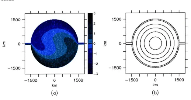
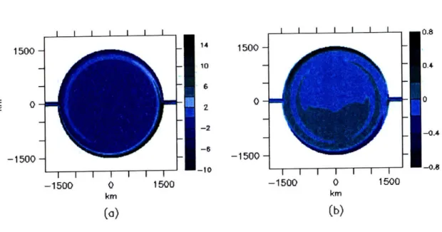
potential vorticity of a water mass exiting the basin, with no net potential vorticity creation inside of the basin. The sea surface height (SSH) contours in Figure 3-1 confirm that in one side of the basin, potential vorticity is added into the basin, and in the other side, an equal amount of potential vorticity is extracted from the basin. Moreover, there is no sign of an intense boundary layer where potential vorticity can be introduced or extracted from the basin.

Basins with unsymmetrical forcing are just as illuminating. The symmetry is broken by tilting the basin such that the sill depths of the inflow and outflow are now at different heights. In this case, the potential vorticity of a water mass entering the basin is different than the potential vorticity of a water mass exiting the basin, producing a net production or net extraction of potential vorticity internally to the basin. I I I I I I II 3 .... 1500 2 0 E 0 -2 -2 -- 1500 -1500 -1500 0 1500 -1500 0 1500 km km

(a)

(b)

Figure 3-1: PV forcing in a symmetric basin: a) SSH b) depth contours

1500-E

0---10 n

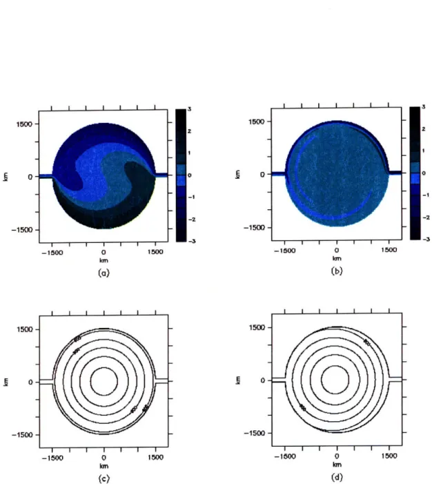
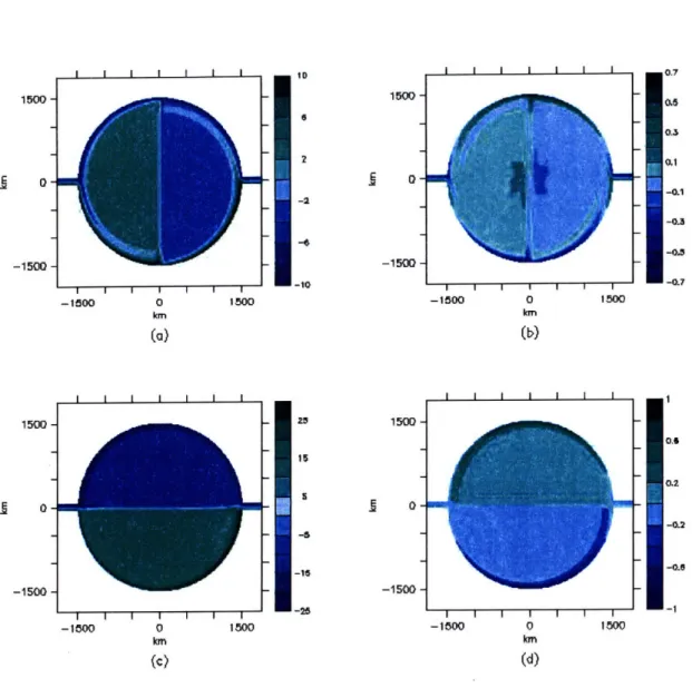
To illustrate this point, the case where the inflow sill depth is deeper than the outflow sill depth will be examined. The PV of the inflow is now smaller than the PV of the outflow which means PV must be introduced into the basin by the only mechanism possible in our model, by horizontal diffusion. We see in Figure 3-2 that the horizontal diffusion of PV into the basin takes place in a strong boundary layer which is limited to only one side of the basin. And contrary to the expected result where a water parcel turns to its right due to the .Coriolis force (in the northern hemisphere), the current turns to its left. This is because a boundary current with a wall on its left diffuses PV from the wall into the boundary current, thus satisfying the PV basin constraint.

This result has direct application to the Arctic Ocean. The Arctic Ocean is rel-atively isolated, with only a few connections to external oceans. Therefore, one can sum the PV of water masses entering and exiting the basin, through the Bering St, Fram St, Barents Sea, Canadian Archipelago, and extract a budget for the net PV entering the basin. There are uncertainties in the mean transport through these pas-sageways, but within uncertainties, there is a net flux of PV into the Arctic, largely because of the large contribution of positive PV by the shallow Bering Strait (r50m vs. -2000 m for the Fram Strait) [16].

If we apply the PV budget to the Arctic, since there is a net flux of PV into the basin from the inflows and outflows, there must also be a negative flux of PV to keep the basin in steady state. As is seen in classical studies of the North Atlantic gyre, the flux of PV must take place in a frictional boundary layer. In the case of a circular basin, this results in a strong boundary layer current with the wall on its right (cyclonic flow) which diffuses negative PV from the frictional boundary layer. This is one possible explanation for the cyclonic circulation of the Arctic circumpolar current.

One drawback to this analysis is that there is no examination of forcing internal to the Arctic. The PV constraint is a broad conservation rule that applies to an entire basin. Some insight can be gained into the interior flow, but it is hard to extract

specifics from such a conservation rule. The PV constraint specifies how water at the boundaries must behave, yet the interior flow rnay take any form.

Yang's [16] study suggests that the potential vorticity of water masses at the gate-ways of the Arctic is the crucial factor for determining the direction of the circulation of the Atlantic Water in the Arctic. Yang examined the case where the transport of water through the gateways was fixed, but the geometry of the basin was varied. The following paper extends Yang's argument by examining the case where the geometry of the basin is fixed, but where the transport of water will vary. In addition, Yang's study solely focused on external forcing by volume transport through the straits. The following paper focuses solely on internal forcing in the form of wind stress at the surface.

1500 o o0 -2 -1500 -1500 0 1500 -1500 0 1500 kmrn kIn (a) (Ib) 1500 E 0 -1500 0 o -1 -2 -1 -1500 0 1500 -1500 0 1500 (c) (d)

Figure 3-2: PV forcing in for a) a symmetric basin b) high PV outflow c) depth contours for symmetric basin d) depth contours for asymmetric basin (tilted so that right is shallower, left is deeper).

1500 G 0 -1500 1500 . 1

0

-1500io -3

.---Chapter 4

Arctic Circulation in an Idealized

Numerical Model

4.1

Introduction

The Arctic Ocean is bounded an ice cap at its surface and by land at its side and bottom. The only contact between the Arctic Ocean and its surrounding seas are

through just a few points - the Bering St., Canadian Archipelago, Fram Strait, and

through the Barents Sea. The only contact between the Arctic Ocean and the atmo-sphere is mediated through a semi-rigid icepack that ranges from tens of meters thick to non-existent thickness.

Observations in the interior Arctic have been limited by the icepack and in the best of times, can be sporadic. Currently, observations are limited to infrequent icebreaker transects, whose routes are guided by leads in the ice pack; therefore repeatable mea-surements in space and time are nearly impossible. These limitations mean that the Arctic circulation is not well known. In addition to the paucity of observations, the variability in the Arctic may be quite large, even on time scales as short as a day [10]. As a result, gleaning the general circulation from CTD casts that are separated in time by hundreds of days and in space by hundreds of kilometers is a challenging

task.

However, a best guess of the present day circulation has been synthesized from available data. The passageways into the Arctic are relatively easy to access, and thus the currents entering and exiting the Arctic are relatively well-sampled and estimates of their magnitude have been made. At the shallow Bering St. [50 in], about 0.8 Sv (Sverdrups) of cold and fresh water enters the Arctic from the Pacific [11]. From the Atlantic, water diverges around Svalbard into Fram St. and the Barents Sea. In the Barents Sea, about 2.2 Sv enters and is transformed, to various degrees, by winter processes like cooling and brine rejection from ice formation, before finally spilling over the shelf into the Arctic Ocean [12]. At the deeper Fram St. [2300 m], warm and salty water from the Atlantic enters the Arctic with a magnitude between 1 and 2 Sv [4].

Upon entering the Arctic, the remnants of the Atlantic water subducts below the fresh and buoyant surface waters of the Arctic and circumnavigate the Arctic Ocean in a cyclonic direction. This Atlantic layer occupies the intermediate depths below the surface waters and above the ridges that subdivide the Arctic Ocean. When the Atlantic layer encounters one of the ridges that bisect the Arctic, the current then appears to split with one branch following the bathymetry into the interior and an-other following the shelf break around the rim towards the Canada Basin. Below the sill height of the ridges, in the deep basins, the water is relatively quiescent with residence times of hundreds of years [13].

Because of the scarcity of observations, numerical models have been used to try to determine the circulation patterns of the Arctic. Many of these models are fully 3D models including ice, realistic bathymnetry, and coupling to the atmosphere. The AOMIP project compared 14 of these numerical models in an attempt to better un-derstand the behavior of Arctic numerical models. A most intriguing finding was the direction of the circulation of Atlantic water: 7 models showed an anticyclonic circulation, and 7 models showed a cyclonic circulation. Each of the models used the same standardized forcing, so such a large anomaly was puzzling.

The likely explanation for this behavior was found by analyzing an idealized Arc-tic basin. Yang [16] studied a homogeneous barotropic model which was forced solely by advection through channels at opposite ends of an Arctic-like basin. Using a basin-wide potential vorticity constraint, Yang showed that the advection of poten-tial vorticity into the basin can control direction of the circulation. By varying the sill depth of the channels, the potential vorticity of the inflow and outflow was mod-ified. Yang's idealized basin was an excellent example of using a simplified model to understand circulation dynamics in the Arctic.

Isachsen and Nost [8] examined the effect of bottom topography on the Arctic cir-culation. They noted that "even the surface flow follows the topographic features". By varying a bottom friction parameter in a numerical model, they found that the integrated effect of the wind stress curl over a closed f/H contour

[f

being the coriolis parameter, H the depth] determines the direction of circulation in the Arctic Ocean and Nordic Seas. Furthermore, they argued that the Arctic circumpolar current was mainly forced by wind stress curl in the Nordic Seas as opposed to the wind stress curl in the Arctic Ocean. This explanation fits in nicely with Yang's simplified model since Yang examined an Arctic model with no internal wind forcing. Instead, the model was indirectly forced by external wind in the form of advection of water through exit and entrance channels.

Bottom topography may be important in the Arctic, but to what extent does it have an effect on the circulation? It has also been shown that vertical stratifica-tion plays an important role in determining how strongly bottom topography affects circulation dynamics. Marshall and Stephens [6] found that in a stratified ocean, the density field baroclinically shields the surface, wind driven circulation from the influence of bottom topography. It is only when topography penetrates above the 'level of density compensation' (halocline in the Arctic, thermocline elsewhere) that topography has an effect on the surface circulation.

Proshutinsky and Johnson [9] used a two-dimensional, barotropic, vertically inte-grated, coupled ice-ocean model to examine the case of a wind-driven Arctic Ocean

that oscillated between anticyclonic and cyclonic circulation regimes on the decadal time-scale. They suggested that the regime shifts are driven by wind. Specifically, by the location and relative magnitudes of high and low pressure systems in the Arctic

- the Icelandic Low and the Siberian High.

Thus there are conflicting ideas on whether eternal forcing or internal forcing drives the circulation of the Arctic Ocean. Internal forces are buoyancy forcing from river outflow, polynyas, or ice formation/melt, but primarily wind stress from the atmosphere. External forcing can be thought of as the net integrated effect of wind forcing external to the Arctic, with the end result of advection of water through nar-row straits into the Arctic.

To date, simplified models have been used to examine the case of external forcing (Nost and Isachsen, Yang), but studies of a simplified Arctic ocean forced primar-ily by wind stress are rare. Newton et al. [7] studied the case of a closed, 2-layer, cylindrical basin and focused on the response of the basin to annular wind modes. However, their focus was on the tilt of the SSH (sea surface height) and pynocline, not on the interior circulation of the Arctic. This study uses an idealized basin to study the effect of internal wind forcing on an Arctic-like basin. In addition, examples with and without ridges and stratification are examined to in order to determine the relative importance of both bottom topography and stratification.

4.2

Model Description

The model geometry used in all calculations is a simplified representation of the Arc-tic, consisting of a circular basin with a bowl shaped bathymetry that has two shallow channels for in and outflows. The model used for our calculations is the primitive equation MITgcm [5]. In each case, the model was run until steady state conditions were reached. As in the Arctic, the coriolis parameter,

f,

was specified to be at a maximum in the center of the basin and decreasing radially. At the walls of the basin, no-slip and no-flux conditions were specified. The horizontal viscosity was set

at 400 m2_{/s and when stratification was included, the vertical diffusivity was set at}

0.01 m2/s and 12 vertical layers were used. The thickness of the layers increased from 25m at the surface to 400m at the bottom. The stratification was introduced by varying the temperature rather than the salinity. This choice for an Arctic-like basin was made because we are only interested in the density stratification. The wind stress, r, has magnitude of 0.04 N2/m.

Ideally, when examining a two-channel basin forced by wind, the transports through the channels would be allowed to vary independently of each other. However, in such a scenario, the volume transport would quickly become unbalanced. In a model with open boundaries, one must choose to either fix the velocity at the boundaries, or al-ternatively, use repeating boundary conditions. However, once the transport is fixed by specifying the velocity at the boundary, then the basin is not fully free to adjust its circulation to internal forcing. The purpose of this study is to examine the effect of the wind on the internal forcing, therefore repeating boundary conditions were used instead of open boundary conditions..

The basin was forced by wind forcing which was constant in time, but varied in strength and orientation: cyclonic, anticyclonic, zonal, and meridional. The main focus of this paper is on the contrast between "zonal" winds (parallel to the channel) and "meridional" winds (perpendicular to the channel).

The same bowl shaped bathymetry was used as in Yang's experiment [16].

R~e- • r<R

H(r) =

0 r>R

where H is the depth of the basin and R is the radius of the basin and equal to 1.5 km. The horizontal resolution was 7.5 km. The channels have straight walls and a width of 112.5 km. For the wind forced runs, the channel depths at each end of the basin are equal (- 450 m). Model runs with unequal channel depth are not possible with the use of repeating boundary conditions.

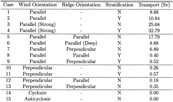
Case Wind Orientation Ridge Orientation Stratification Transport (Sv) 1 Parallel - N 8.88 2 Parallel - Y 10.84 3 Parallel (Strong) - N 25.68 4 Parallel (Strong) - Y 32.79 5 Parallel Parallel N 17.79

6 Parallel Parallel (Deep) N 8.88

7 Parallel Perpendicular N 6.89 8 Parallel Parallel Y 0.40 9 Parallel Perpendicular Y 0.52 10 Perpendicular - N 0.26 11 Perpendicular - Y 0.57 12 Perpendicular Parallel N 0.18 13 Perpendicular Perpendicular N 0.35 14 Cyclonic - N 0.00 15 Anticyclonic - N 0.00

Table 4.1: Parallel and Perpendicular refer to the orientation of wind/ridges relative to the channel. For wind orientation, "Strong" means 3 times the strength of normal forcing. For ridge orientation, "Deep" refers to a deep ridge at depth of 860m, if unspecified, the ridge is equal to the depth of the channel. All parameters are time invariant.

Ridges were introduced to examine the effect of bathymetry on the circulation. The ridges bisect the basin and are orientated in two directions; parallel or perpen-dicular to the channels. The ridges have vertical walls and are equal in width to the channels. The depth of the ridges are either "shallow" and equal to the depth of the channels, or they are "deep" and located at a depth of 860 meters. In either case, the ridges have the same width as the channels.

4.3

Results

4.3.1

Wind Forcing

With the introduction of wind, the simplest case is a basin forced by a uniform zonal wind (Figure 4-1). In this case, no PV is introduced into the basin and there should be no net production or dissipation of PV in this basin. The net result is a SSH

buildup in the direction of the wind and an antisymmetric distribution of velocity which cancels out any PV diffusion through the boundary of the basin.

The next case is an open basin which is forced by both along-channel and cross-channel wind (Figure 4-2). These two examples illustrate how a 90 degree shift in wind direction can produce a large change in the circulation of the basin. In the case of the along-channel wind, a sharp boundary current is produced, and the channel through-flow is 8.88 Sv. In the case of cross-channel wind, there is a dramatically smaller transport through the channel (0.26 Sv), resulting in a circulation which looks remarkable similar to the closed basin. The dramatic reduction of transport can be explained by comparing the open basin model runs to the closed basin model run. If we examine the SSH of the closed basin with "zonal" wind (Figure 4-la), then introduce channels on the right and left, this would have the effect of introducing two channels at the point where the SSH height difference in maximum. So when the channels are added, the SSH gradient can be relaxed and a strong channel transport results (Figure 4-2a).

On the other hand, if we again examine a closed basin with "zonal" wind but now introduce channels on the top and bottom. This has the effect of adding two channels at the point where the SSH height difference is at a minimum. With SSH being nearly equilibrated, when the channels are added, there is now almost no channel transport (Figure 4-2b). A basin forced by cyclonic and anticyclonic winds was also examined (Figure 4-3). In these cases, the wind forcing is parallel to f/H contours and easily to excite flow along f/H contours. Note that there is no strong boundary layer in the cyclonic or anticyclonic wind scenarios. Instead, the velocity slowly increases radially from the center of the basin. However, there is now a net diffusion of PV into the basin through the wide frictional boundary layer in either case due to the anticyclonic and cyclonic circulation. This compensates the PV input from the wind so that the basin-wide budget of PV is conserved.

1000 - 0--1000 ---- 0.5 cm/s I I I I I I I I 1.2 0.8 1000-0,.4 0 0--0.4 -1000 -0.8 K I I 1 I I I "I 1 I I -1000 0 1000 -1000 0 1000 km km

(b)

(c)

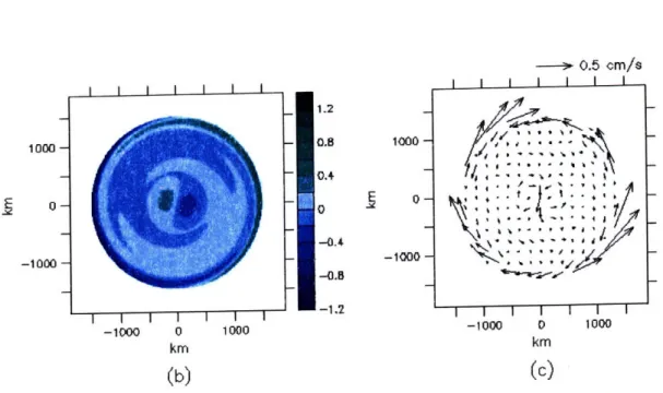
Figure 4-1: Wind forcing on a closed basin a) SSH b) Velocity vectors of the flow in the basin

:I

r

//( ... Y-rcc | I | | I I | I | | | | • • I I | • | • •

-14 1500 10 2 0 2 -2 -1500 -1500 0 1500 -1500 0 1500

(a)

(b)

Figure 4-2: SSH for an open basin with a) along channel wind b) cross channel wind

1500

-1500

4

-0.4

1500 -1500 -1500 0 1500 km -- * lv cm/s I I I 1 o I I I 1500 1500-E 0 -1500--1500 0 1500 km 10c Is I I -1500I -1500 I I I I I 0 1500

Figure 4-3: Annular wind forcing in an open basin a) SSH for cyclonic wind b) SSH for anticyclonic wind c) velocity for cyclonic wind d) velocity for anticylonic wind

1500 0 -1600 150 0--1500 --1500

\I$I

I I ... .. -"

4.3.2

Addition of Bathymetry (Ridges)

To which degree do f/H contours affect the circulation? We addressed this by adding a ridge to the basin, and forcing it with the same variation of winds as in the previous cases. The depth and width of the ridge is equal to the depth and width of the channel and is orientated either parallel or perpendicular to the channel. This results in two symmetric sets of closed f/H contours, one on each side of the basin, divided by the ridge.

In the case with cross-channel and along-channel winds, the only significant change comes where the wind, channel, and ridge are all aligned in the same direction (Figure 4-4c). There is now a strong current flowing in the center of the basin, following the ridge. With the addition of this ridge, the net transport through the channel is doubled from 8.9 Sv (no ridge) to 17.8 Sv (with ridge). The doubling of transport results from the addition of another f/H contour which facilitates the flow of water from one end the basin to the other. This extra f/H contour (the ridge) has a volume transport of almost 10 Sv, accounting for the large increase in transport. Away from the ridge and boundaries, the basin is nearly quiescent.

In the model run with the ridge perpendicular to both the wind and the channel (Figure 4-4a), the addition of a ridge does not significantly change the circulation compared to the model runs without a ridge. There is now a slight transport along the ridge, but the channel transports are still of the same magnitude, with about a 25% reduction in transport through the strait (compared to the same case with no ridge). In this orientation, the ridge does not facilitate transport through the channels; instead it impedes the boundary currents which are the only pathways capable of transporting water from one end of the basin to the other. This model orientation resembles the real bathymetry of the Arctic Ocean. In the Arctic Ocean, the Lomonosov Ridge transects the Arctic roughly perpendicularly to the Bering and Fram Straits with its shallowest point at about 1000m.

I I I I I I I 1500--1500 --1500 0 1500 k(c (C) 1500 0 -1500 0-oa -1500--1500 0 1500 km (b) I- I I I I I 1 I -13000 I I 0 1500 km( (d)

Figure 4-4: Wind forcing in an open basin with ridges. SSH for: a) along channel wind and cross channel ridge b) cross channel wind and cross channel ridge c) along channel wind and along channel ridge d) cross channel wind and along channel wind

4.3.3

Effect of Stratification

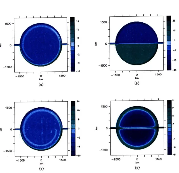
Stratification is a necessary addition to our model in order to study whether the density field blocks the effect of f/H contours. There is not much change in basins without ridges once stratification is added. But when the basins with ridges are examined, a large shift is seen. In these cases, the stratification drastically affects the circulation. In the case with wind, channel, and ridge aligned (Figure 4-5d),

1 0 I I I I -1500 0 1500 km (a) 1500 -1500 IM

the transport through the channel shrinks from 17.8 Sv to 0.4 Sv compared to the barotropic case (Figure 4-5b), almost a 50-fold reduction in magnitude. In addition, where there was once a calm interior (Figure 4-5b) there is now an interior circulation created in the basins on either side of the ridge.

The main reason for this dramatic reduction of transport is made clear by closely examining the currents around the ridge. In the unstratified case, there is only uniform current. However in the stratified case, on either side of the ridge is an opposing current with volume transport each of about 1.5 Sv. This is because there are now two cyclonic gyres set-up, one on either side of the ridge. This is similar to the case of the Arctic where there are opposing currents on either side of the Lomonosov Ridge with corresponding cyclonic gyres in the surrounding basins.

I I I I I I I -1-00 0 1500 kmI 1500 E 0 -1500 0 1500 krn I I I I I I I I I I 1500 2 E 0 -2 -4 -1500 -1500 0 1500 km (d)

Figure 4-5: Along channel wind forcing in an open basin comparing the effects of ridges and stratification. SSH for a) Control run (unstratified, no ridge) b) Unstrati-fied with a shallow ridge c) UnstratiUnstrati-fied with a deep ridge d) StratiUnstrati-fied with a shallow ridge 0 01500 - 1500- -10--1500 -S " T I T T I -1500 0 1000 km (c) N

4.4

Discussion and Conclusions

Newton et al. [7] examined an idealized Arctic-like basin forced solely by annular

winds. This study also examines an idealized Arctic basin forced by zonal or merid-ional winds. In both cases it was found that the winds can modulate the SSH gradient which will affect the transport of water between the Arctic Ocean and its surrounding oceans. In this paper, it was shown that a 90 degree shift in wind direction, from zonal to meridional (or vice versa), can shut off or intensify transport through the channels by modulating the SSH at the boundaries.

Our model was forced with basin-scale winds and reached steady state after 100 days (much sooner in most cases). When forced with winds parallel to the channels, the channel transport was found to be 10 Sv. However, when forced with perpendic-ular wind, the transport was reduced 0.5 Sv. And when forced with an annperpendic-ular wind, there was no transport through the channels. This is in contrast to the measured flow in the Bering Strait of 0.8 Sv, the inflow at the Barents Sea of 2 Sv, and at the Fram St. of 1.2 Sv. This result shows that internal wind forcing can play a dominant role in setting the circulation of the Arctic. An average wind stress was applied in the along channel direction and a channel transport an order of magnitude larger than the observed mean transport through the Bering St. was created.

This is no mere theoretical exercise as observations show that it is possible for the transport between the Arctic and its surrounding seas to the greatly modulated by the wind. In the Bering St., it is believed that the mean flow of about 0.8 Sv is primarily due to a pressure head difference between the Arctic and Pacific' Oceans. Transport due to wind forcing is then super-imposed on top on the mean flow (the annual mean wind opposes the mean flow [15]). Observations from moorings in the Bering St. show that local winter storm events are strong enough to not just shut off the flow through the channel, but reverse the transport for days at a time. This shows that local wind events may not merely shut off the flow, but also reverse the flow in a shallow channel.

A more relevant question to climate is whether these shifts in wind occur at longer time-scales and at larger spatial scales. Do large-scale Arctic SLP (sea level pressure) patterns vary at seasonal, annual, or decadal time-scales? How closely do they re-semble our zonal and meridional winds? Figure 4-6 shows the Arctic SLP (sea level pressure) for the mean of July and August for 4 consecutive years (1993-1996). The contrast between 1995 and 1996 is most noticeable. In both years the geostrophic wind is directly along the Fram St., but there is nearly a 180 degree shift in SLP in the span of one year. In 1995, the geostrophic wind points out of the Arctic, but in 1996, the geostrophic wind is directed into the Arctic. The effect of these large-scale pressure variations was quite dramatic. In 1995 an abnormally large ice export was

recorded but in 1996 an abnormally small ice export was recorded.

In addition to the 90 degree shift of winds, it was also found that bathymetry (in the form of ridges) and stratification play a role in setting the circulation of the Arctic Ocean. Figure 4-5 shows the contrast between a barotropic basin without ridges (a), a barotropic basin with a shallow ridge (b), a barotropic basin with a deep ridge (c), and a stratified basin with a shallow ridge (d).

The effect of bathymetry can be examined by contrasting the first three barotropic cases. With the addition of a ridge, there are now closed f/H contours that cross the interior of the basin (Figure 4-7). In the case of the shallow ridge, those closed contours add a direct path from one end of the basin to the other enable an increased transport. But in the case of a deep ridge, the closed contours are formed deeper, in the quiet interior of the basin. There is no new path a water parcel may follow into the interior basin and therefore the deep ridge and the no-ridge runs are nearly identical.

The effect of stratification can be examined by contrasting the barotropic shallow ridge and the stratified shallow ridge cases (Figures 4-5b, 4-5d). The most visible difference is the net transport through the channels: 17.8 Sv in the barotropic case, 0.4 Sv in the stratified case. In the stratified case, as opposed to the barotropic case, there is no large transport from one end of the basin to the other. Instead, the ridge separates two currents moving in opposite direction, a more realistic scenario that is similar to the circulation patterns near the Loinonosov ridge.

This study, although highly idealized, has similarities to the real Arctic Ocean. There are only a few relatively narrow channels connecting the Arctic to the out-side world, the Lomonosov ridge bisects the Arctic (roughly perpendicularly to the Bering and Fram Straits), and atmospheric pressure patterns have been observed to have a time variability ranging from days to decades (and most likely unobserved for centuries, millennia, etc.). There is a need for more idealized models that can shed light on the underlying dynamics of the Arctic circulation. They are an underutilized tool which can not only be used to explain the behavior of more complex numerical models, but also the behavior of the real Arctic Ocean.

b) Jul/Aug 1994

1006 1006 1010 1012 1014 t016 101 I 0o2o

Sea level pressure, mbar

0low 100o Io6 1012

Sea level pressure, mbar

) Jul/Aug c 1995

d) ul/Aug 1996

IM04 1006 1000 1010 1012 1014 101 100 1006 1007 l00 10lll 1013 101t

Sea level pressure, mbar Sea level pressure, mbar

Figure 4-6: Mean SLP in the Arctic for July and from NCEP/NCAR reanalysis project.

August from 1993-1996. Data taken

__ ) )1I1/A•n 100q ~~ rut -r ---- l----o -r 00C

I I I I I I -1000 0 1000 1000 --1000 -(b) I I I I I I -1000 0 1000 (b)

Figure 4-7: f/H contours in and open basin with a) no ridges b) shallow ridge

I I I I

0-·-L

1000 -E107_-0

_-I

--100OO -i I111II

Chapter 5

Conclusion

There are many tools physical oceanographers may use to attack the complex prob-lem of ocean geophysical fluid dynamics. The tool that is chosen must fit the goal of the study. Scientists who study the problem of how much temperatures may rise in future climates must necessarily use the only tool available - fully coupled global models. The goal of this study is much less ambitious and so the tool that is chosen is an idealized numerical model. With this simpler approach, "real forecasts" are sacrificed to gain understanding of a small piece of the puzzle of ocean dynamics.

This study took the approach of stripping away much of the extraneous details to look at the fundamental dynamics of the system. Thus, the difficult task was to avoid introducing too many variables which might clutter the experiment while at the same time devising experiments which would allow insight into the underlying dynamics. In every experiment, bathymetry was kept symmetric and winds were always uniform in both space and time. Among the most significant missing variables were the ice cover, atmospheric heat flux, freshwater cycles, and time-varying winds.

This idealized numerical model complements rather than competes with highly complex numerical models. An intriguing next step to this study would pair this ide-alized numerical model with an intermediate-to-high complexity model. Both models

stratifica-tion - but the more complex model would use realistic Arctic bathymetry and an ice cover. This would check to what extent the dramatic shift in regimes between stor-age and transport that we saw in the idealized model takes place in a more realistic setting.

Appendix A

Additional figures

I I I I I I I

g

1500 -E 0--1500 --1500 -II U I I I I I I /U 1500 50 30 10 E 0 -10 -30 -50 -1500 -70 -1500 0 1500 -1500 0 1500 km km

(a)

(b)

Figure A-1: Anticyclonic wind forcing for a basin with a) normal magnitude winds

b) strong magnitude winds (3x normal)

Discussion: The SSH response to strengthening wind is nearly linear; a three-fold increase in wind stress corresponds to a three-fold increase in SSH. In addition, you can see the effect of a wind which is parallel to f/H contours on the magnitude of the SSH. Compared to the cases with wind parallel/perpendicular to the channels, the anticyclonic SSH is 1-2 orders of magnitude larger.

150 50 --50 -150 I --250

1500 -E 0--1500 -I I I I I I I I I I I -1500 0 1500 12 1500 a E 0 -1500 -1500 0 1500

(a)

(b)

Figure A-2: Cyclonic wind with a shallow ridge parallel to the channels: a) SSH b) depth contours

Discussion: In this case, bathymetry has a large effect on the circulation. The shallow ridge blocks the free flow along circular f/H contours. The result is a stagnant interior and a slight SSH build-up windward of the ridge.

I I

1500 -E 0- -1500-- 1500 -1500--I 14 I 150U -10 6 E 0 -2 -6 1500 -50 30 10 -10 -50 -r•0 I I I I I I I I I I 1 -1500 0 1500 -1500 0 1500 km km

(a)

(b)

Figure A-3: Wind forcing parallel to the channels in an open basin with a) normal strength winds b) strong winds (3x normal)

Discussion: Again, the response to wind is nearly linear (3x wind - 3x SSH). In the case with the strong winds, the velocity shear between the boundary current and interior is large enough so that eddies can be seen to be shedding. The plotted SSH is in quasi-steady state. a m -| ll |1 | | l | A| | | 0_ 1 I - ~ -' a s I I I I I I I I I I I I

I I I I I I I 1500 5 0 -1500 I I I I I I I -1500 0 1500 kln (a) I I I I I I I I I I I -1600 0 kmn (c) I I 1500 1500 0 -1500 1500 --1500 -i I I 0 I 1 I -1500 0 1500 kmn (b) I I I I I I I km (d)

Figure A-4: Wind forcing parallel to the channels in an open basin with ridges of varying orientation: a) shallow ridge parallel to channels b) deep ridge parallel to channels c) shallow ridge perpendicular to channels d) deep ridge perpendicular to channels

Discussion: The first thing to notice is that the right-hand plots are practically iden-tical. In fact, they are also nearly identical to figure A-3(a). The deep ridges have no effect on the circulation because they do not interact with the strong boundary cur-rents. The next thing to notice is the large effect the shallow ridges have on the SSH. The shallow ridges are level with the channels, thus they interact with the boundary current and unnaturally divide the basin into two halves with alarmingly differenct

SSH. 1500-1 o1500

-L

I

-1500 0 1500 M M I I M1 1 I I I I I 1 I I

1500 1500 -- 0--1500 -I -I -I -I -I -I -I

S I I I I

I

-15W0 0 1500 km I I I I I 1500 -I 0--1500 -I I I I I I I -1500 0 1500 km (c) -1500 1500-S O1500 --1500 0 1500 km (b) I I I I -1500 0 1500 km (d)

Figure A-5: Wind forcing perpendicular to channels in an open basin with varying ridge orientations: a) shallow ridge parallel to channels b) deep ridge parallel to channels c) shallow ridge perpendicular to channels d) deep ridge perpendicular to channels

Discussion: Same as figure A-4, but with wind forcing perpendicular to the channels instead of parallel to the channels. Again, the deep ridges have negligible effect on the circulation, while the shallow ridges have a much larger effect.

M

i

1500 - 0- -1500-I I I I I I I I I I I I I I -1500 0 1500 km

(a)

1.2 0.8 0.4 -0.4 -0.8 -1 1 1500 -E 01500 -I I I I I I I -1500 0 1500 km

(b)

Figure A-6: Zonal wind forcing in a closed basin: a) homogeneous b) stratified

Discussion: This is the simplest experiment set-up; a uniform zonal wind in a closed basin, thus an ideal test case for the first run with stratification. All is well as the SSH is nearly identical between the homogeneous and stratified basins.

1.2 0.8 0.4 0 -0.4 -0.8 -1.2 I I 1 I I I I

.-18 14 10 6 -2 40 20 D -W0 -1500 0 1500 -1500 0 Io0 kmrn km (o) (b) 150 1500 7 1 -1 -1500 1 7 5 3 _ -l -3 -100 0 1800 -100 0 1800 km km (c) (d)

Figure A-7: Wind forcing parallel to channels in a stratified basin: a) normal winds

b) strong winds (3x normal) c) normal winds with a ridge parallel to channels d)

normal winds with a ridge perpendicular to channels

Discussion: Again, the strong wind case has a SSH about 3x the SSH of the normal wind case. The new feature to notice is the symmetry of the SSH in the case with ridges. Compare figure A-7(c,d) to figure A-4(a,c). Without stratification, there is just a single, strong jet confined to the ridge. But the addition of stratification enables currents on either side of the ridge to flow in opposite directions, exactly what is seen near the Lomonosov Ridge.

E

1500

-1500

Bibliography

[1] K. Aagaard and L.K. Coachman. Towards an ice-free arctic ocean.

Transactions-American Geophysical Union, 56(7):484-486, 1975.

[2] R.G. Barry, M.C. Serreze, and et al. Maslanik, J.A. The arctic sea-ice climate

sys-tem -observations and modeling. Reviews of Geophysics, 31(4):397-422,

Novem-ber 1993.

[3] International Council for Science (ICSU). A framework for the international polar year 2007-2008 produced by the icsu ipy 2007-2008 planning group. Technical report, 2004.

[4] E.P. Jones. Circulation in the arctic ocean. Polar Research, 20(2):139-146, 2001. [5] J. Marotze, R. Giering, and et al. Zhang, K.Q. Construction of the adjoint mit ocean general circulation model and application to atlantic heat transport sensitivity. Journal of Geophysical Research-Oceans, 104(C12):29529-29547, Dec

15 1999.

[6] David Marshall and James Stephens. On the insensitivity of the wind-driven cir-culation to bottom topography. Journal of Marine Research, 59(1):1-27, January 2001.

[7] B Newton, L.B. Tremblay, and et al. Cane M.A. A simple model of the arctic ocean response to annular atmospheric modes. Journal of Geophysical

Research-Oceans, 111(C9):C09019, Sep 15 2006.

[8] Ole Nost and P ' 1 Isachsen. The large-scale time-mean ocean circulation in the nordic seas and arctic ocean estimated from simplified dynamics. Journal of

Marine Research, 61(2):175-210, March 2003.

[9] AY Proshutinsky and M Johnson. Two circulation regimes of the wind driven arctic ocean. Journal of Geophysical Research-Oceans, 102(C8):12493-12514, Jun 15 1997.

[10] L. Rainville and P. Winsor. Mixing across the arctic ocean: Microstructure observations during the beringia 2005 expedition. Geophysical Research Letters, 35(8):L08606, Apr 30 2008.

[11] A.T. Roach, K. Aagaard, and et al. Pease, C.H. Direct measurements of transport and water properties through the bering strait. Journal of Geophysical

Research-Oceans, 100(C9):18443-18457, Sep 15 1995.

[12] B. Rudels, E.P. Jones, and et al. Schauer, U. Atlantic sources of the arctic ocean surface and halocline waters. Polar Research, 23(2):181--208, 2004.

[13] P. Schlosser, B. Kromer, and et al. Ekwuezel, B. The first trans-arctic c-14 section: Comparison of the mean ages of the deep waters in the eurasian and canadian basins of the arctic ocean. Nuclear Instruments and Methods in Physics

Research Section B-Beam Interactions with Materials and Atoms,

123(1-4):421-437, March 1997.

[14] Mary-Louise Timmermans and Chris Garrett. Evolution of deep water in the canada basin in the arctic ocean. Journal of Physical Oceanography, 36(5):866--874, May 2006.

[15] R.A. Woodgate and K. Aagaard. Revising the bering strait freshwater flux into the arctic ocean. Geophysical Research Letters, 32(2):L02602, Jan 20 2005. [16] J.Y. Yang. The arctic and subarctic ocean flux of potential vorticity and the

arctic ocean circulation. Journal of Physical Oceanography, 35(12):2387-2407, December 2005.