Publisher’s version / Version de l'éditeur:
Journal of Alloys and Compounds, 422, 1-2, pp. 164-172, 2006
READ THESE TERMS AND CONDITIONS CAREFULLY BEFORE USING THIS WEBSITE. https://nrc-publications.canada.ca/eng/copyright
Vous avez des questions? Nous pouvons vous aider. Pour communiquer directement avec un auteur, consultez la première page de la revue dans laquelle son article a été publié afin de trouver ses coordonnées. Si vous n’arrivez pas à les repérer, communiquez avec nous à [email protected].
Questions? Contact the NRC Publications Archive team at
[email protected]. If you wish to email the authors directly, please see the first page of the publication for their contact information.
NRC Publications Archive
Archives des publications du CNRC
This publication could be one of several versions: author’s original, accepted manuscript or the publisher’s version. / La version de cette publication peut être l’une des suivantes : la version prépublication de l’auteur, la version acceptée du manuscrit ou la version de l’éditeur.
For the publisher’s version, please access the DOI link below./ Pour consulter la version de l’éditeur, utilisez le lien DOI ci-dessous.
https://doi.org/10.1016/j.jallcom.2005.11.068
Access and use of this website and the material on it are subject to the Terms and Conditions set forth at
Small step graphs of cell data versus composition for ccp
solid-solution binary alloys: application to the (Pt,Ir), (Pt,Re) and (Pt,Ru)
systems
Le Page, Y.; Bock, C.; Rodgers, J. R.
https://publications-cnrc.canada.ca/fra/droits
L’accès à ce site Web et l’utilisation de son contenu sont assujettis aux conditions présentées dans le site LISEZ CES CONDITIONS ATTENTIVEMENT AVANT D’UTILISER CE SITE WEB.
NRC Publications Record / Notice d'Archives des publications de CNRC:
https://nrc-publications.canada.ca/eng/view/object/?id=f069db44-f49a-4713-9535-9340c6b2c25c https://publications-cnrc.canada.ca/fra/voir/objet/?id=f069db44-f49a-4713-9535-9340c6b2c25cSmall step graphs of cell data versus composition for ccp solid-solution
binary alloys: Application to the (Pt,Ir), (Pt,Re) and (Pt,Ru) systems
Y. Le Page
a,∗, C. Bock
a, J.R. Rodgers
baM12, ICPET, National Research Council of Canada, Ottawa, Ont., Canada K1A 0R6 bToth Information Systems Inc., Ottawa, Ont., Canada K1J 6B2
Received 2 November 2005; received in revised form 25 November 2005; accepted 29 November 2005 Available online 15 February 2006
Abstract
It is shown here that crystallographic descriptions of hypothetical AB63, AB107, AB127, AB215and especially AB255stoichiometric compounds with cell edge, respectively 4, 3, 4, 6 and four times the (A,B) fcc subcell edge stick out as convenient models for ab initio studies of cell data versus composition for ccp solid-solution alloys. Their Wyckoff positions can be combined to generate most binary alloy compositions from 0% to 100% in multiples of 1/64, 1/108, 1/128, 1/216 and 1/256 while retaining the same periodicity and, respectively the same Fm¯3m, Pm¯3m, Im¯3m, Fm¯3m and Pm¯3m space group symmetry. As an application, we model cell data for three cubic solid-solution alloys of Pt. (Pt,Ir) and (Pt,Ru) remain close to Vegard’s law predictions with a slight convexity or concavity in the plot. That curvature is explainable by the magnitude and sign of the alloying energy. Modeling of (Pt,Re) between 0% and 45% Re in 50 steps of RenPt108−n stoichiometric compounds follows approximately non-Vegard
experimental data but with large, unexplained spread. The method has been automated in Materials Toolkit (http://www.tothcanada.com/toolkit). © 2006 Published by Elsevier B.V.
Keywords: Intermetallics; Computer simulations; Fuel-cells
1. Introduction
Current fuel-cell research efforts hinge on the catalytic prop-erties of a variety of platinum alloys, most of which are close-packed solid-solutions, either ccp or hcp. Experimental cell data for a few solid-solution alloys are well documented in the litera-ture, while those for others are not. Sometimes, reported values turn out to be insufficiently precise or samples insufficiently characterized. It is then tempting to complement the existing experimental data with some modeling, either to support the data, fill composition gaps or clarify deviations from Vegard’s law (Vegard[1]; Thorpe and Garboczi[2]).
We contributed before to the characterization of the slope of Vegard’s law in (Pt,Ru) cell data (Bock et al.[3]). Ab ini-tio modeling of cell data for solid-soluini-tion systems is performed by optimizing cell and coordinate data for hypothetical stoichio-metric compounds within the known range of the solid-solution. This optimization is the essence of the Car and Parrinello[4]
∗Corresponding author. Tel.: +1 613 993 2527.
E-mail address:yvon.le [email protected] (Y. Le Page).
algorithm. This algorithm, which is implemented in all density functional theory (DFT) packages, is at the base of the current explosion of applications of DFT to materials science and chem-istry problems. It is well known that DFT quantum modeling can extract correctly tiny energy or stress differences between two models, while the value itself of that energy or stress may be affected by a much larger bias. This is why for example the rou-tine calculation of accurate elastic coefficients for crystalline materials is feasible in the presence of a pressure bias that is commonly a GPa or so even with today’s best pseudopotentials. Adequate precautions are therefore required in order to perform most modeling operations. If at all feasible, the atomic content of the primitive cell, the Cartesian components of its cell edges, the symmetry, the origin of atom coordinates and the k-mesh should be identical from simulation to simulation. For execution speed, symmetry should also be as high as possible. In the present con-tribution, we try to optimize the production of cell data versus composition plots around the above criteria. In performing this analysis, we somewhat extrapolate on what is economically fea-sible today with coarse steps and extend the analysis toward finer steps that will be reasonably achievable in 5–10 years provided that Moore’s law goes on holding for that length of time.
0925-8388/$ – see front matter © 2006 Published by Elsevier B.V. doi:10.1016/j.jallcom.2005.11.068
Table 1
Possible models with holohedral cubic symmetry for ab initio simulation of ccp alloys
Type Wyckoff site Site symmetry Atom coordinates
(a) Formula: AB7, Z = 4, Space group: Fm¯3m, a = 2asubcella
A 4a m¯3m 0 0 0
B 4b m¯3m 1/2 0 0
B 24d m·mm 0 1/4 1/4
(b) Formula: AB26, Z = 4, Space group: Fm¯3m, a = 3asubcellb
A 4a m¯3m 0 0 0
B 24e 4m·m 0.333333333 0 0
B 32f ·3m 0.333333333 0.333333333 0.333333333
B 48h m·m2 0 0.166666667 0.166666667
(c) Formula: AB63, Z = 4, Space group: Fm¯3m, a = 4asubcellc
A 4a m¯3m 0 0 0 B 4b m¯3m 1/2 0 0 B 8c ¯43m 1/4 1/4 1/4 B 24d m·mm 0 1/4 1/4 B 24e 4m·m 0.250000000 0 0 B 48h m·m2 0 0.125000000 0.125000000 B 48i m·m2 1/2 0.375000000 0.375000000 B 96k ··m 0.125000000 0.125000000 0.250000000
(d) Formula: AB124, Z = 4, Space group: Fm¯3m, a = 5asubcelld
A 4a m¯3m 0 0 0 B 24e 4m·m 0.400000000 0 0 B 24e 4m·m 0.200000000 0 0 B 32f ·3m 0.200000000 0.200000000 0.200000000 B 32f ·3m 0.400000000 0.400000000 0.400000000 B 48h m·m2 0 0.100000000 0.100000000 B 48h m·m2 0 0.200000000 0.200000000 B 96j m·· 0 0.200000000 0.400000000 B 96k ··m 0.400000000 0.400000000 0.200000000 B 96k ··m 0.300000000 0.300000000 0.400000000
(e) Formula: AB215, Z = 4, Space group: Fm¯3m, a = 6asubcelle
A 4a m¯3m 0 0 0 B 4b m¯3m 1/2 1/2 1/2 B 24d m·mm 0 1/4 1/4 B 24e 4m·m 0.333333333 0 0 B 24e 4m·m 0.166666667 0 0 B 32f ·3m 0.166666667 0.166666667 0.166666667 B 32f ·3m 0.333333333 0.333333333 0.333333333 B 48g 2·mm 0.166666667 1/4 1/4 B 48h m·m2 0 0.166666667 0.166666667 B 48h m·m2 0 0.083333333 0.083333333 B 48i m·m2 1/2 0.333333333 0.333333333 B 48i m·m2 1/2 0.416666667 0.416666667 B 96j m·· 0 0.083333333 0.250000000 B 96k ··m 0.083333333 0.083333333 0.333333333 B 96k ··m 0.083333333 0.083333333 0.166666667 B 192l 1 0.250000000 0.166666667 0.083333333
(f) Formula: AB31, Z = 1, Space group: Pm¯3m, a = 2asubcellf
A 1a m¯3m 0 0 0 B 1b m¯3m 1/2 1/2 1/2 B 3c 4/mm·m 0 1/2 1/2 B 3d 4/mm·m 1/2 0 0 B 12i m·m2 0 0.250000000 0.250000000 B 12j m·m2 1/2 0.250000000 0.250000000
(g) Formula: AB107, Z = 1, Space group: Pm¯3m, a = 3asubcellg
A (Atom 1) 1a m¯3m 0 0 0 B (Atom 2) 3c 4/mm·m 0 1/2 1/2 B (Atom 3) 6e 4m·m 0.333333333 0 0 B (Atom 4) 6f 4m·m 0.333333333 1/2 1/2 B (Atom 5) 8g ·3m 0.333333333 0.333333333 0.333333333 B (Atom 6) 12h mm2·· 0.166666667 1/2 0 B (Atom 7) 12i m·m2 0 0.333333333 0.333333333 B (Atom 8) 12i m·m2 0 0.166666667 0.166666667
Table 1 (Continued )
Type Wyckoff site Site symmetry Atom coordinates
B (Atom 9) 24l m·· 1/2 0.333333333 0.166666667
B (Atom 10) 24m ··m 0.166666667 0.166666667 0.333333333
(h) Formula: AB255, Z = 1, Space group: Pm¯3m, a = 4asubcellh
A 1a m¯3m 0 0 0 B 1b m¯3m 1/2 1/2 1/2 B 3c 4/mm·m 0 1/2 1/2 B 3d 4/mm·m 1/2 0 0 B 6e 4m·m 0.250000000 0 0 B 6f 4m·m 0.250000000 1/2 1/2 B 8g ·3m 0.250000000 0.250000000 0.250000000 B 12h mm2·· 0.250000000 1/2 0 B 12i m·m2 0 0.125000000 0.125000000 B 12i m·m2 0 0.250000000 0.250000000 B 12i m·m2 0 0.375000000 0.375000000 B 12j m·m2 1/2 0.125000000 0.125000000 B 12j m·m2 1/2 0.250000000 0.250000000 B 12j m·m2 1/2 0.375000000 0.375000000 B 24k m·· 0 0.125000000 0.375000000 B 24l m·· 1/2 0.125000000 0.375000000 B 24m ··m 0.125000000 0.125000000 0.250000000 B 24m ··m 0.375000000 0.375000000 0.250000000 B 48n 1 0.375000000 0.250000000 0.125000000
(i) Formula: AB15, Z = 2, Space group: Im¯3m, a = 2asubcelli
A 2a m¯3m 0 0 0
B 6b 4/mm·m 0 1/2 1/2
B 24h m·m2 0 0.250000000 0.250000000
(j) Formula: AB127, Z = 2, Space group: Im¯3m, a = 4asubcellj
A 2a m¯3m 0 0 0 B 6b 4/mm·m 0 1/2 1/2 B 8c ·¯3m 1/4 1/4 1/4 B 12d ¯4m·2 1/4 0 1/2 B 12e 4m·m 0.250000000 0 0 B 24h m·m2 0 0.125000000 0.125000000 B 24h m·m2 0 0.250000000 0.250000000 B 24h m·m2 0 0.375000000 0.375000000 B 48i ··2 1/4 0.375000000 0.125000000 B 48j m·· 0 0.125000000 0.375000000 B 48k ··m 0.125000000 0.125000000 0.250000000
aCompositions not achievable: (3, 4)/8.
b Compositions not achievable: (2, 3, 4, 5, 10, 11)/27. cCompositions not achievable: (5, 11, 17, 23, 29)/64.
d Compositions not achievable: (2, 3, 4, 5, 10, 11, 16, 17, 22, 23, 28, 29, 34, 35, 40, 41, 46, 47, 52, 53, 58, 59)/125. eCompositions not achievable: (3, 4, 5, 11)/216.
fCompositions not achievable: (9, 10, 11)/16. g Compositions not achievable: (2, 5)/108.
h All compositions that are integer multiples of 1/256 are achievable. i Compositions not achievable: (2, 5, 6, 7, 8)/16.
j Compositions not achievable: 2/128.
2. Optimal computational models
As shown below, all the above general precautions can be implemented in modeling of cell data versus alloy composition apart, of course, from the atomic content of the primitive cell. However, difficulties arise that are detailed below.
2.1. Sufficiently fine composition steps
A first difficulty arises with the composition step. If we want a composition step s, the primitive cell of our model must then
contain at least 1/s atoms. As we want s to be as small as possible, this means that our model must include many atoms. However, optimization of models becomes very slow above 70 atoms or so, depending on the symmetry. In the particular case of ccp solid-solutions, the maximum symmetry of compositional models is holohedral cubic. Preserving this cubic symmetry is then crucial for the optimizations to be feasible at all with 100 or more atoms per primitive cell, which is required for percent composition steps. We are then restricted to building n × n × n supercells of one of three possible primitive cells: the 60◦rhombohedron of
109.54◦rhombohedron built by body centering the cube of the
2 × 2 × 2 supercell. No other holohedral cubic solution can exist. As the fcc rhombohedron contains one atom, its supercells with cubic symmetry then contain 1 × n3with n integer, i.e. 8, 27, 64, 125, 216, 343, 512, etc. atoms. The cube contains four atoms and its supercells then contain 32, 108, 256, 500, etc. atoms. The bcc rhombohedron contains 16 atoms and its supercells 128, 432, 1024, etc. atoms. The possibly useful and tractable numbers in the above list are 8, 16, 27, 32, 64, 108, 125, 128, 216 and 256. Simulations for the last five numbers of atoms are barely feasible with PCs today, but as they will presumably become tractable in just a few years, we include them in the analysis below. The next number, 343, is likely to remain both out-of-reach for a while, and of limited usefulness anyway.
2.2. Achievable compositions
A second difficulty is the alloy compositions that can be achieved while retaining holohedral cubic symmetry. The prob-lem boils down to combinations of the multiplicities of the occupied Wyckoff positions. This problem is easily handled with the Supercells and Symmetry tools in Materials Toolkit (Le Page and Rodgers[5];http://www.tothcanada.com/toolkit/). In Table 1, we accordingly report the cubic crystallographic descriptions for hypothetical AB7, AB15, AB26, AB31, AB63,
AB107, AB124, AB127, AB215 and AB255 stoichiometric ccp
compounds. AB7, AB15, AB26 and AB31, respectively shown
inTable 1a, i, b and f all combine the drawbacks of coarse com-position steps with huge gaps in the achievable comcom-positions. AB124(Table 1d) turns out to be a poor choice because it
dis-plays both drawbacks of a relatively large number of atoms per primitive cell as well as significant gaps in the compositions that are achievable by selecting full occupancy at its Wyckoff positions by either just element A or just element B. In compar-ison, models based on the Wyckoff positions of AB63in Fm¯3m
(Table 1c) then seem to constitute the compromise between sufficiently fine composition step (1.56%) and affordable com-puting effort. They do not allow generation of fractions 5, 11, 17, 23, 29, 35, 41, 47, 53 and 59/64, but those are equally spaced numbers, leaving no big composition gap empty or depleted. Similarly, AB107, AB127and AB215inTable 1g, j and e appear
to be acceptable selections, leaving only a few gaps for low percentage alloying, but otherwise covering nicely the interme-diate range with no gaps. Finally, AB255 (Table 1h) seems to
be an excellent selection for the future, as it leaves no compo-sition gap at all. Quantum optimizations involving 256 atoms with cubic symmetry are expensive today, but they will no longer be by 2010 provided that Moore’s law holds until that date.
2.3. Degree of randomness
An ideal solid-solution displays randomness of its atom dis-tribution, a fact translating in reciprocal space by a clean powder diffraction pattern of the simple structure type for the element, usually ccp or hcp, with no additional lines, not even diffuse ones. No periodic superstructure can be claimed to be random,
Table 2
Bonds per cell with first neighbours for each atom position inTable 1g are given as a row Atom # 1 2 3 4 5 6 7 8 9 10 1 12 2 12 24 3 24 24 24 4 24 24 24 5 24 48 24 6 24 24 24 24 48 7 12 24 12 48 48 8 12 24 12 48 48 9 24 24 48 24 48 72 48 10 24 24 48 48 48 48 48
Both rows and columns are in the order ofTable 1g. The cell contains 648 bonds, each linking two atoms. Each bond is then counted twice in the table.
but some periodic distributions are further remote from ran-domness than others. For example, the ratios of the numbers of AA:AB:BB bonds in a random distribution of composition (AxB1−x) are x2:2x(1 − x):(1 − x)2. We then attempt to create
superstructure models that approximate those proportions as closely as feasible. In the following discussion, we use the mate-rial AB107inTable 1g as an example.Table 2shows in its cells
the number of bonds per crystallographic cell linking atom i and its symmetry equivalents to atom j and its equivalents as numbered inTable 1g.Table 2was produced by multiplication of the number of bonds originating from each atom as printed by the Distances and Angles tool in Materials Toolkit by the multiplicity of that atom printed in Table 1g. Apart from the compositions 1, 3, 4, 104, 105 and 107/108 for which there is no leeway in the selection of the atoms from the list giv-ing the correspondgiv-ing total number of atoms per cell, all other achievable compositions can be obtained through multiple selec-tions. For example, composition 6/108 can be achieved in two ways, by selecting either atom #3 or atom #4. Those two ways are not equivalent because it can be read off Table 2that the first generates no AA bond, 72 AB bonds and 576 BB bonds, while the second one generates 24 AA bonds, 48 AB bonds and 576 BB bonds. As the numbers expected from the random distribution of a composition in the proportion of six atoms A and 102 atoms B are 2:68:578, it is clear that the first selec-tion approximates more closely a random distribuselec-tion than the second one. Composition 9/108 can be achieved in three ways, by involving atom numbers (2,3), (2,4) and (1,5). Each time, we select that distribution of atoms which best approximates the distribution of bonds expected from a random distribution of atoms in the same atomic proportion. We report inTable 3
the optimum solution for the various achievable compositions. In most cases, several distributions achieve the same sum of the squares of the differences in numbers of AA, AB and BB bonds. We did not implement any additional criterion in the selection of the printed optimum solution. In order to fully implement the structures described in the various Table 1a–i, readers should then build the corresponding neighbour tables, similar toTable 2here, and implement considerations above as inTable 3.
Table 3
Optimum occupancy by atom A of the various atom sites inTable 1g leading to alloy formula ANB108−Nwhile minimizing the sum of the squares of the differences
in numbers of AA, AB and BB bonds with respect to a random distribution of atoms A and B with same proportions
N Occupancy of the 10 sites inTable 1g Sqrt of sum of square
of differences 1 2 3 4 5 6 7 8 9 10 1 1 – – – – – – – – – 0.136 3 – 1 – – – – – – – – 1.225 4 1 1 – – – – – – – – 2.177 6 – – 1 – – – – – – – 4.899 7 1 – 1 – – – – – – – 6.668 8 – – – – 1 – – – – – 8.709 9 1 – – – 1 – – – – – 11.023 10 1 1 1 – – – – – – – 13.608 11 – 1 – – 1 – – – – – 16.466 12 – – – – – 1 – – – – 9.798 13 1 – – – – 1 – – – – 6.396 14 – – 1 – 1 – – – – – 26.672 15 – 1 – – – 1 – – – – 1.225 16 1 1 – – – 1 – – – – 5.443 17 – 1 1 – 1 – – – – – 39.328 18 – – – 1 – 1 – – – – 14.697 19 1 – – 1 – 1 – – – – 9.662 20 – – – – 1 – – 1 – – 4.355 21 – 1 – 1 – 1 – – – – 1.225 22 1 1 – 1 – 1 – – – – 7.076 23 – 1 – – 1 – – 1 – – 13.200 24 – – – – – – – – 1 – 9.798 25 1 – – – – – – – 1 – 3.130 26 – – – 1 1 – 1 – – – 3.810 27 – 1 – – – 1 – 1 – – 11.023 28 1 1 – – – 1 1 – – – 10.887 29 – 1 – 1 1 1 – – – – 3.130 30 – – – 1 – – 1 1 – – 4.899 31 1 – 1 – – – – – – 1 13.200 32 – – – – 1 – – – – 1 21.773 33 – 1 1 – – – – – 1 – 1.225 34 1 1 1 – – – – – 1 – 10.342 35 – 1 1 1 1 1 – – – – 9.662 36 – – 1 1 – – – – 1 – 0.000 37 1 – – – – 1 – – 1 – 9.934 38 – – 1 – 1 – – – 1 – 9.254 39 – 1 – – – – – 1 1 – 1.225 40 1 1 – – – 1 – – – 1 11.975 41 – 1 – 1 1 – – – – 1 22.998 42 – – – 1 – – – 1 1 – 4.899 43 1 – – 1 – 1 – – 1 – 12.928 44 – – – – 1 1 – – – 1 1.089 45 1 – – – 1 1 – – – 1 11.023 46 1 1 – 1 – – – 1 – 1 5.988 47 – 1 – – 1 – – 1 – 1 6.668 48 – – 1 1 – 1 – – 1 – 9.798 49 1 – 1 1 – – – 1 1 – 3.402 50 – – 1 – 1 1 – – 1 – 12.520 51 1 – 1 – 1 – – 1 1 – 1.225 52 1 1 1 1 – – – 1 1 – 14.153 53 – 1 1 – 1 – – 1 1 – 0.136 54 – – 1 – – 1 1 – 1 – 14.697
Atom B occupies the sites denoted with a minus sign for easy legibility.
3. The cubic solid-solution alloys (Pt,Ir), (Pt,Re) and (Pt,Ru)
The alloys (Pt,Ir), (Pt,Re) and (Pt,Ru) are currently the subject of intense studies aiming at the optimization of their catalytic
activity and resistance to poisoning in fuel-cell operation. How-ever, literature data for the characterization of these alloys using cell edge versus composition information remains spotty or in need of clarifications. We therefore attempt to apply the above considerations to the calculation of detailed cell data versus
com-position graphs based on the experimental observation that those alloys are ccp solid-solutions.
3.1. (Pt,Ir)
Both Pt and Ir are ccp elements. Cell data versus composi-tion for (Pt,Ir) have been studied by Raub[6]and by Tripathi and Chandrasekharaiah[7]who report data for 13 compositions each. Tripathi reports significant deviations from Vegard’s law, with the worst deviations under 50% Ir, but Raub’s data points in this range follow rather nicely Vegard’s straight line.
3.2. (Pt,Ru)
Gasteiger, Ross and Cairns[8]report numerical cell data val-ues for four ccp alloys in the Pt–Ru system. They do not comment on the behaviour, but their data fits nicely on a straight line. For Ru content greater than 80%, the alloys are hcp. Bock et al.[3]
report an ab initio low-resolution plot of the a cell edge versus Ru content, also plotting on a straight line with same slope as the experimental data. Strictly speaking, this straight line cannot be called Vegard’s law because pure Ru is hcp. It is nevertheless interesting to note that the extrapolation of the straight line to pure Ru gives a cubic cell volume with precisely twice the vol-ume of the hcp experimental cell, as it should. We nevertheless reinvestigate the (Pt,Ru) system at higher resolution in order to contrast the behaviour of the three alloy systems.
3.3. (Pt,Re)
The alloys of Pt and Re were studied using powder diffrac-tion by Trzebiatowski and Berak[9]who report curves of cell data versus Re content. Their main conclusions are that they form cubic solid-solutions up to about 40% Re without obeying Vegard’s law. Rhenium itself is hcp and its alloys with Pt remain hcp down to about 60% Re. Both phases coexist in the region from 40% to 60% Re. We accurately digitized the data points in theirFig. 2. In view of the lasting importance of this work 50 years later, we print their results inTable 4below, includ-ing the hcp data. We transformed their results from kX units and rescaled them to aPt= 3.9231 ˚A reported by Swanson and
Tatge[10], which is probably still the most reliable cell edge value for Pt at 25◦C. Grgur, Markovic and Ross[11]as well as
Rudman[12]report individual cell data–Re content pairs that more-or-less fit on Trzebiatowski and Berak’s curve.
4. Modeling and results 4.1. Modeling parameters
In order to compare meaningfully simulation results, the VASP execution parameters must be preserved from run to run. For all simulations within this study, we used the following parameters.
We performed computations with VASP.4.6.4[13]on both Linux and Windows machines with medium-precision calcula-tions using GGA PAW[14]potentials, electronic convergence
Table 4
Cell data for (Pt,Re) alloys, accurately digitized fromFig. 2in Trzebiatowski and Berak[9]and rescaled to a = 3.9231 ˚A for pure platinum at 25◦C (Swanson
and Tatge,[10])
Re (%) Cubic a Hexagonal a Hexagonal c
0 3.9231 2.5 3.9195 5 3.9172 7.5 3.9151 10 3.9127 20 3.9076 30 3.9020 35 3.9012 40 3.8990 45 3.8986 2.7668 4.4314 50 3.8982 2.7670 4.4322 55 3.8982 2.7668 4.4317 60 2.7672 4.4272 70 2.7681 4.4181 80 2.7734 4.4193 90 2.7659 4.4355 95 2.7637 4.4465 100 2.7625 4.4596
Re values rescaled to Pt in this way also agree very well with 25◦C values for
Re in Swanson and Fuyat[18].
at 10−7eV level and energy cutoff 260 eV. The convergence for forces was 10−4eV/ ˚A. A Methfessel–Paxton[15]smearing scheme was used, with order 1 and width 0.2 eV. Calculations did not include spin polarization. A maximum of 40 SCF cycles were used per single point while 30 single points ensured conver-gence. Davidson’s[16]blocked scheme was used in combination with reciprocal projectors. We used a uniform 2 × 2 × 2 k-mesh with a Monkhorst–Pack scheme[17].
4.2. Calculation of the bond energy difference ε for alloying
Under the rough assumption that the cohesive energy U of an (AxB1−x) alloy is stored in its AA, AB and BB bonds,
solid-solutions exist when the energy UABof the bond linking an atom
of type A and an atom of type B is approximately the average of UAAand UBB, which can be written
2UAB= UAA+ UBB+2ε (1)
Provided that |ε| is smaller than kT at alloy formation temper-ature, the elements will then display miscibility, but without formation of defined compounds where element A surrounds itself with element B and vice-versa. They lead instead to materials known as solid-solution alloys. Combined with the
x2:2x(1 − x):(1 − x)2 distribution for, respectively AA:AB:BB bonds, Eq.(1)leads after rearrangement to
U = N(x2UAA+(1 − x)2UBB+ x(1 − x)(UAA+ UBB+2ε))
from which,
U = N(−2εx2+(UAA− UBB+2ε)x + UBB) follows, (2)
where N is the number of interatomic bonds per supercell. As the coefficient of the quadratic term is −2Nε, it follows
that the alloying energy ε can be read off as −a/2N in the quadratic fit U = ax2+ bx + c obtained by least-squares regres-sion of the experimental total energy data U versus the alloy composition x.
Derivation of cell data for RePt107is then a matter of
request-ing cell and structure optimization based on the crystallographic description ofTable 1h to VASP and running the computing job. With VASP.4.6 running on an AMD Athlon 64 built beginning of 2005 and operated under Windows XP, and a 2 × 2 × 2 k-mesh corresponding to 0.04 ˚A−1reciprocal resolution, the execution time is about 1 week. We felt that a 1 × 1 × 1 k-mesh would be too coarse for a metallic system while a 3 × 3 × 3 k-mesh would lead to computation times that would be inordinately long. In spite of the borderline feasibility today, we decided to go ahead and implement the general method in Section 1 in the hope that, owing to Moore’s law, the automated derivation of cell-composition graphs for ccp binary solid-solutions using modest computing equipment will be quite convenient as close as 5 years from now.
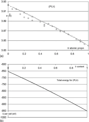
Fig. 1. (a) Cell data vs. Ir content x for (Pt1−xIrx) system. Triangles: Raub (1959); circles: Tripathi and Chandrasekharaiah (1983); plus signs: this work. Although superficially looking like a textbook case of Vegard’s law, the calculated data actually displays a slight convexity, probably due to the item below. In order to clearly see the convexity after reduction for journal requirements, readers may have to look down the line, at an angle to the page. (b) Calculated values for the total energy per cell vs. Ir content for (Pt1−xIrx) alloys. The convexity is quite perceptible and due to the fact that the energy associated with a Pt–Ir bond is slightly higher than the average for a Pt–Pt bond and an Ir–Ir bond.
5. Results 5.1. Pt1−xIrx
Cell data results are shown in Fig. 1a and total energy results inFig. 1b. The ab initio cell data were corrected for the expected bias originating in approximations common to all DFT packages. The bias is known from the very accurate cell data measurements for pure Pt and Ir [10]. This linear rescaling was by a factor 0.9888 at Pt and 0.9900 at Ir. The Vegard-law fit is: a (Pt1−x,Irx) = 3.9222 − 0.0714x − 0.0114x2
applicable to all values of x from 0 to 1. The “Vegard slope” is then −0.0714 − 0.0228x, corresponding to −0.0714 at Pt while it is −0.0942 at Ir. The least-squares fit to the energy data is
U= −30.721x2−266.82x − 653.75, meaning that alloying cor-responds to an energy of +24 meV per AB bond.
5.2. Pt1−xRux
Cell data results are shown in Fig. 2a and total energy results in Fig. 2b. The Vegard-law fit is: a (Pt1−x,Rux) =
Fig. 2. (a) Calculated cell data vs. Ru content x for (Pt1−xRux) system. This time, the calculated data actually displays a very slight concavity, seen clearly on full-page plots and extracted accurately by least squares, but probably difficult to see after the required size reduction. (b) Total energy per simulation cell for Pt1−xRuxalloys. The data displays a slight concavity due to the fact that the energy of a Pt–Ru bond is very slightly lower than the average of a Pt–Pt and a Ru–Ru bond.
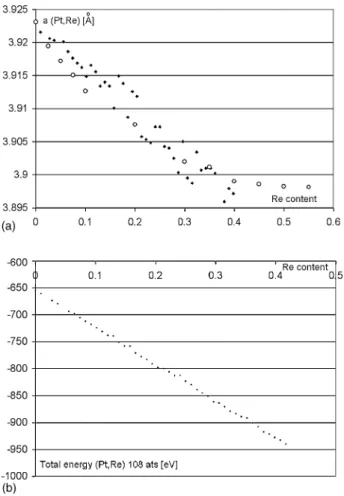
Fig. 3. (a) Calculated cell data vs. Re content x for (Pt1−xRex) system. The cal-culated data displays considerable spread. Circles are Trzebiatowski and Berak’s [11]data points over the ccp region for (Pt,Re). (b) Total energy per simulation cell for Pt1−xRexalloys. Contrary to cell data inFig. 3a, the energy plot displays no big spread and virtually no curvature.
3.9231 − 0.1489x applicable to all values of x from 0 to about 0.8 because it is experimentally known that (Pt,Ru) alloys are in fact hcp in the range 0.8 < x ≤ 1. The least-squares fit to the energy data is U = +11.536x2−339.04x − 652.08, meaning that alloying corresponds to an energy of −8.9 meV per AB bond.
5.3. Pt1−xRex
Calculations were performed in the range 0 ≤ x < 0.45 because the (Pt,Re) alloys are known to be hcp in the range 0.6 < x ≤ 1, ccp in the range 0 ≤ x < 0.4 and two-phased for 0.4 < x < 0.6. The plot of cell edge versus x shown inFig. 3a displays considerable spread while roughly following the gen-eral trend indicated by experimental data. We performed those simulations using different starting points and obtained each time comparable spread with different data points. In view of the poor quality of plot 3a, we leave it to readers to derive their own conclusions. In contrast, the plot of the total energy U does not display any anomaly. The least-squares fit to the energy data is U = 3.465x2−686.67x − 654.39 in eV, indicating a very small energy difference of −2.7 meV per AB bond.
6. Discussion
The (Pt,Ir) and (Pt,Ru) results are quite well behaved and in agreement with experimental results. The curvature of the total energy plot is very noticeable for (Pt,Ir), which also displays a small but significant deviation of cell data with respect to Veg-ard’s law. As far as we know, this small curvature of the cell data is a new observation. In fact, Raub’s[6]triangles onFig. 1a fol-low remarkably well the calculated data points from this work and could be interpreted as an experimental observation of the curvature. We feel that the two observations of the curvature of the energy and of the cell data versus composition are related and explainable as indicated below.
In a situation where ε would be zero, the alloy would be random, the plot of U versus x would be straight and Vegard’s law would be accurately obeyed. The convexity of the plot of U versus x indicates that the energy of two AB bonds is greater than that of an AA bond plus a BB bond. In other words, the elements A and B are at a slight energy disadvantage if they mix than if they stay separate. However, this repulsion is overcome by the thermal energy kT at alloy formation time. Annealing at lower temperatures might cause nanoscale segregation within the alloy, but that would require very long times, and may not happen at room temperature due to the energy barrier for diffusion that is much higher than the small energy to be gained. At any rate, in the range of compositions around 50% Ir, the (Pt,Ir) is at a slight energy disadvantage with respect to an alloy for which ε would be zero because half of its bonds are AB bonds. An alloy with ε= 0 would follow Vegard’s law. A slight lengthening of the a cell edge with respect to Vegard’s law is then expected around 50% Ir because of the weaker cohesive energy. It is seen here clearly for the first time as a slight convexity in the plot of a versus x.
The opposite situation is seen on a smaller scale with Ru. Contrary to Ir, Ru has a very slight energy advantage to mix with Pt. A slight concavity in the plot of a versus x is then expected and observed here, but it is so slight that it could easily be missed.
The case of (Pt,Re) alloys is inconclusive for three reasons. First the curvature of the plot of U verses x is about three times smaller than for Ru, meaning that the expected devia-tion from Vegard’s law would be barely noticeable. Second, our data extends only in the range 0 ≤ x < 0.45, where the curvature would be more difficult to see than in the full range from 0 to 1. The third and main reason is the large and unexplained spread in ab initio cell data. Additional convergence cycles did not fix this spread. Starting with a different cell edge or nudging atoms with respect to ideal fractional positions produced slightly different converged cell edges, a fact for which we have no explanation because we proceeded in exactly the same way as for Ir and Ru which did not display any such spread.
7. Conclusion
We systematized here a way to model cell edge versus finely stepped composition for ccp solid-solution binary alloys and implemented it as an automated tool in Materials Toolkit
(http://www.tothcanada.com). We applied this software to the (Pt,Ir), (Pt,Ru) and (Pt,Re) systems that are known to be solid-solution binary alloys. The corresponding jobs were distributed for execution among two Linux clusters and one 8-CPU Win-dows setup, all with VASP.4.6.4 running on state-of-the-art Intel or AMD CPUs.
Results for (Pt,Ir) and (Pt,Ru) indicate that Vegard’s law is followed quite well, but with a previously unnoticed slight con-vexity or concavity that we relate here to, respectively a small positive or negative alloying energy. The ability to model binary alloys with small composition steps without altering the cell data or the space group symmetry was crucial in order to disclose this kind of small deviation with respect to Vegard’s law.
Results for (Pt,Re) are consistent with experimental data, but with a wider spread for which we hope that DFT package devel-opers will find a cure.
The above piece of work required a lot of computing time on many CPUs. In this respect, it may be somewhat ahead of what is easily feasible today, but assuming that Moore’s law would hold for another 5 years, all computing times would be divided by a factor 10, making this type of work quite tractable with much more modest equipment.
Acknowledgements
We wish to thank Ron Jerome from ICPET for his com-petent creation and management of the “idletime” queue on ICPET’s cluster that made this huge computation possible by using only idle cycles on all nodes of the cluster, thus without getting in the way of high-priority daytime use. We also thank NRC’s Research Computing Support Group, in particular Wayne
Podaima, Doug Ritchie and Michel Proulx for fast access to the high-performance computing queue as well as competent help and support.
References
[1] L. Vegard, Z. Phys. 5 (1921) 17–26.
[2] M.F. Thorpe, E.J. Garboczi, Phys. Rev. B 42 (1990) 8405–8417. [3] C. Bock, B. Macdougall, Y. Le Page, J. Electrochem. Soc. 151 (2004)
A1268–A1278.
[4] R. Car, M. Parrinello, Phys. Rev. Lett. 55 (1985) 2471–2474. [5] Y. Le Page, J.R. Rodgers, J. Appl. Cryst. 38 (2005) 697–705. [6] E. Raub, J. Less-common Metals 1 (1959) 3–18.
[7] S.N. Tripathi, M.S. Chandrasekharaiah, J. Less-common Metals 91 (1983) 251–260.
[8] H.A. Gasteiger, P.N. Ross, E.J. Cairns, LEIS and AES on sputtered and annealed polycrystalline Pt–Ru bulk alloys, Surf. Sci. 293 (1993) 67–80.
[9] W. Trzebiatowski, J. Berak, Bulletin de l’acad´emie polonaise des sciences, Classe Troisi`eme 2 (1954) 37–40.
[10] H.E. Swanson, E. Tatge, Natl. Bur. Std Circ. 539 I (1953) 31.
[11] B.N. Grgur, N.M. Markovic, P.N. Ross, Electrooxidation of H2, CO and
H2/CO mixtures on a well-characterized Pt–Re bulk alloy electrode and
comparison with other Pt binary alloys, Electrochim. Acta 43 (1998) 3631–3635.
[12] P.S. Rudman, J. Less-Common Metals 12 (1967) 79–81. [13] G. Kresse, Thesis, Technische Universit¨at Wien, 1993;
G. Kresse, J. Hafner, Phys. Rev. B 48 (1993) 13115–13118; G. Kresse, J. Hafner, Phys. Rev. B 49 (1994) 14251–14269. [14] G. Kresse, J. Joubert, Phys. Rev. B 59 (1999) 1758–1775. [15] M. Methfessel, A.T. Paxton, Phys. Rev. B 40 (1989) 3616–3621. [16] E.R. Davidson, in: G.H.F. Diercksen, S. Wilson (Eds.), Methods in
Com-putational Molecular Physics NATO Advanced Study Institute, Series C, vol. 113, Plenum, New York, 1983, p. 95.
[17] H.J. Monkhorst, J.D. Pack, Phys. Rev. B 13 (1976) 5188–5192. [18] H.E. Swanson, R.K. Fuyat, Natl. Bur. Std. Circ. 539 II (1953) 13.