Key comparison CCEM-K7: AC voltage ratio

(1)

Publisher’s version / Version de l'éditeur: Metrologia, 49, Technical Supplement, 2011-05-20

READ THESE TERMS AND CONDITIONS CAREFULLY BEFORE USING THIS WEBSITE. https://nrc-publications.canada.ca/eng/copyright

Vous avez des questions? Nous pouvons vous aider. Pour communiquer directement avec un auteur, consultez la première page de la revue dans laquelle son article a été publié afin de trouver ses coordonnées. Si vous n’arrivez pas à les repérer, communiquez avec nous à PublicationsArchive-ArchivesPublications@nrc-cnrc.gc.ca.

Questions? Contact the NRC Publications Archive team at

PublicationsArchive-ArchivesPublications@nrc-cnrc.gc.ca. If you wish to email the authors directly, please see the first page of the publication for their contact information.

NRC Publications Archive

Archives des publications du CNRC

This publication could be one of several versions: author’s original, accepted manuscript or the publisher’s version. / La version de cette publication peut être l’une des suivantes : la version prépublication de l’auteur, la version acceptée du manuscrit ou la version de l’éditeur.

For the publisher’s version, please access the DOI link below./ Pour consulter la version de l’éditeur, utilisez le lien DOI ci-dessous.

https://doi.org/10.1088/0026-1394/49/1A/01007

Access and use of this website and the material on it are subject to the Terms and Conditions set forth at Key comparison CCEM-K7: AC voltage ratio

Robinson, Ian; Belliss, Janet; Bryant, Stephen; Sánchez, Antonio; Álvarez, Yolanda; Schweiger, Kurt; Díaz, Carlos; Neira, Miguel; Callegaro, Luca; Lee, Rae Duk; Blanc, Isabelle; Overney, Frederic; He, XiaoBing; Ding, Cheng; Qian, ZhongTai; Waltrip, Bryan; Small, Greig; Fiander, John; Coogan, Peter; Johnson, Heather Leigh; Nakamura, Yasuhiro; Dierikx, Erik; Saxena, Anil Kishore; Saleem, Mohd; Wood, Barry; Ramm, Guenther; Eklund, Gunnar; Turhan, Enis; Semenov, Yuri

https://publications-cnrc.canada.ca/fra/droits

L’accès à ce site Web et l’utilisation de son contenu sont assujettis aux conditions présentées dans le site LISEZ CES CONDITIONS ATTENTIVEMENT AVANT D’UTILISER CE SITE WEB.

NRC Publications Record / Notice d'Archives des publications de CNRC:

https://nrc-publications.canada.ca/eng/view/object/?id=3d471dc2-249f-4bdd-9a23-ffcf325da7b8 https://publications-cnrc.canada.ca/fra/voir/objet/?id=3d471dc2-249f-4bdd-9a23-ffcf325da7b8

(2)

Key Comparison CCEM-K7 :

AC Voltage Ratio

Draft B Report - Version I - Part 1

May 20, 2011

Ian Robinson1, Janet Belliss1, Stephen Bryant1, Antonio Sánchez2, Yolanda Álvarez2_{, Kurt Schweiger}2_{, Carlos Díaz}2_{, Miguel Neira}2_,

Luca Callegaro3, Rae Duk Lee4, Isabelle Blanc5, Frederic Overney6, XiaoBing He7, Cheng Ding7, ZhongTai Qian7, Bryan Waltrip8, Greig Small9, John Fiander9_{, Peter Coogan}9_{, Heather Leigh Johnson}9_{, Yasuhiro Nakamura}10_,

Erik Dierikx11, Anil Kishore Saxena12, Mohd Saleem12, Barry Wood13, Guenther Ramm14, Gunnar Eklund15, Enis Turhan16, Yuri Semenov17

This report provides the results of a key comparison, CCEM-K7, organised under the auspices of the Comité Consultatif d’Électricit´e et Magnétisme (CCEM) and carried out by a group of National Metrology Institutes (NMIs). The mea-sured parameters were a set of ratios of a type of voltage transformer called an Inductive Voltage Divider (IVD). A single custom-made IVD - the Travelling Standard- was designed and used specifically for this comparison.

Participating Laboratories:1_NPL† 2_CEM3_IEN4_KRISS5_LNE6_METAS7_NIM8_NIST 9_NMIA10_NMIJ11_VSL12_NPLI13_NRC14_PTB15_SP16_UME17_VNIIM

†_{Pilot Laboratory: NPL, Hampton Road, Teddington, Middlesex, TW11 0LW UK}

(3)

List of Tables

1 CCEM-K7 Participants . . . 4 2 Calibration Schedule . . . 5

1 Introduction

Many nations have signed up to a Mutual Recognition Arrangement (MRA) to improve and simplify trade amongst themselves. The MRA process is controlled by the Comité Interna-tional des Poids et Mesures (CIPM) formed from delegates to the Conférence Genéral des Poids et Mesures (CGPM) which is itself comprised of delegates from countries that are signatories to the Convention du Metré.

One of the key points of the MRA is mutual recognition of measurement capabilities be-tween nations. In order to facilitate this process, the CIPM and the Bureau International des Poids et Mesures (BIPM) have organised a series of key comparisons between the National Metrology Institutes (NMIs) with electrical measurements organised under the auspices of the Comité consultatif d’ Électricité et Magnétisme (CCEM).

2 Organisation

2.1 Organisation

The comparison was started as proposal No. CCE/97-31, put to the 21st_{session of the CCE}1

in June 1997 by Ian Robinson (NPL) and through discussion between interested parties lead to a informal meeting at CPEM ’982_{, held in Washington D.C. , USA}

The Pilot Laboratory for key comparison CCEM-K7 was the National Physical Laboratory (NPL) UK : NPL’s role was to

• Prepare and disseminate the Technical Protocol document to participants; • Coordinate the testing schedule ;

• Organise the despatch and return of the Travelling Standard between participant and pilot laboratory, or between participants as required;

• Collect, archive and analyse the reported data;

• Prepare and disseminate the Draft A and Draft B Reports

1_{Consultative Committee on Electricity - renamed CCEM in 1997} 2_{Conference on Precision Electromagnetic Measurements}

(5)

2.2 Participants

Table 1 lists all participants in CCEM-K7 ( arranged in alphabetical order of Identifier) Table 1: CCEM-K7 Participants

Identifier Name Country (RMO)a

CEMb Centro Español de Metrologia Spain EUROMET

IEN Istituto Elettrotecnico Nazionale Galileo

Ferraris Italy EUROMET

KRISS Korea Research Institute of Standards

and Science Korea, Republic of APMP

LCIE Laboratoire Central des Industries

Elec-triques France EUROMET

METASc Metrology and Accreditation Switzerland Switzerland EUROMET

NIM National Institute of Metrology China APMP

NISTd National Institute of Standards and

Tech-nology USA

NMIAe National Measurement Institute Australia APMP

NMIJf National Metrology Institute of Japan Japan APMP

NMi-VSL Nederlands Meetinstituut - Van Swinden

Laboratorium The Netherlands EUROMET

NPL National Physical Laboratory United Kingdom EUROMET

NPLI National Physical Laboratory of India India APMP

NRC National Research Council Canada SIM

PTB Physikalisch-Technische Bundesanstalt Germany EUROMET

SP SP Technical Research Institute of

Swe-den Sweden EUROMET

UMEg Tubitak Ulusal Metrologi Enstitüsü Turkey MENAMET

VNIIMh D.I. Mendeleyev Institute for Metrology Russian Federation COOMET

a_{Regional Metrology Organisation} b_{Joined 2001-01} c_{formerly OFMET} d_{Withdrew in 2000-11; re-joined in 2002-08} e_{formerly CSIRO-NML} f_{formerly ETL} g_{Joined 2001-10} h_{Joined 2001-01} 4

(6)

2.3 Testing Schedule

The initial plan called for all testing to be completed within a 2 year period using an 8-week cycle of 2 weeks for despatch between laboratories , 4 weeks for testing at the participant laboratory and another 2 weeks for despatch back to the pilot laboratory. At the commence-ment of the comparison the schedule was heavily loaded towards the latter half of the project, leaving large gaps in the 1st _{year and no spare capacity the 2}nd _year.

At the beginning of the 2nd _{year, the program was extended to be over 3 years duration.}

This decision was made because of numerous delays caused by shipment problems, 3 new laboratories joined the comparison and several participants requested an opportunity to re-measure.

The pilot laboratory was responsible for the arrangement and cost of the outward journey to participant laboratories - the participant laboratory was responsible for the arrangement and cost of the return or onward journey.

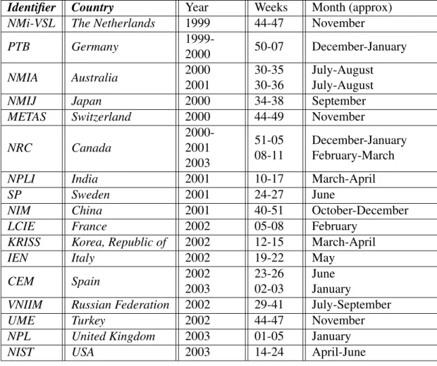
Table 2: Calibration Schedule

Identifier Country Year Weeks Month (approx) NMi-VSL The Netherlands 1999 44-47 November PTB Germany 1999-2000 50-07 December-January NMIA Australia 2000 2001 30-35 30-36 July-August July-August NMIJ Japan 2000 34-38 September METAS Switzerland 2000 44-49 November NRC Canada 2000-2001 2003 51-05 08-11 December-January February-March NPLI India 2001 10-17 March-April

SP Sweden 2001 24-27 June

NIM China 2001 40-51 October-December LCIE France 2002 05-08 February

KRISS Korea, Republic of 2002 12-15 March-April

IEN Italy 2002 19-22 May

CEM Spain 2002 2003 23-26 02-03 June January

VNIIM Russian Federation 2002 29-41 July-September UME Turkey 2002 44-47 November NPL United Kingdom 2003 01-05 January NIST USA 2003 14-24 April-June

(7)

3 Calibration Artefact & Shipping

3.1 The Travelling Standard

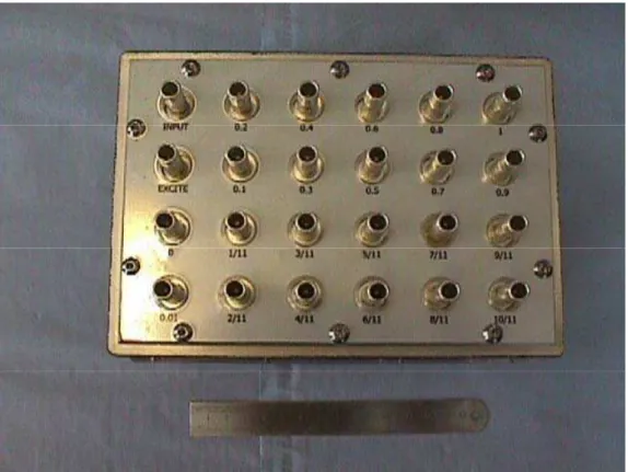
A custom-made IVD was designed and constructed specifically for the comparison by Greig Small and John Fiander of NMI, Australia [1] and delivered to NPL in June 1999. The IVD is a 2-stage design with fixed output taps for 10-section ( i.e. decade), 11-section and 0.01 ratio windings. Figure 1 is a schematic of the IVD. All connections are made via BPO (MUSA) coaxial sockets on the top panel of the divider. The outer terminals of all the coaxial connectors except the EXCITE terminal are connected in parallel, by direct contact to the copper slab that forms the top panel. The IVD dimensions are approximately (length x width x height) 175 x 125 x 145 mm (165 mm including MUSA sockets) and net weight is 4.90 kg. It fits snugly within a red wooden box that comes in two parts, so the lid can be removed for access to the terminals and the IVD can be left within the lower box. The box parts join up via 8 long screws through the edges of the lid. The box dimensions are 195 x 155 x 195 mm. A tamper-proof seal was applied to one of the torx screws holding the transformer to the metal case at the beginning of the programme. It remained intact until intentionally broken at the pilot laboratory in January 2002. It was re-sealed and remained intact until the end of the programme.

(8)

1 2 3 4 A B C D 4 3 2 1 D C B A Title Number Revision Size A4

Date: 29-Sep-1998 Sheet of File: I:\pc\cce_ivd\windings.sch Drawn By:

0 1/11 2/11 3/11 4/11 5/11 6/11 7/11 8/11 9/11 10/11 1 1/10 2/10 3/10 4/10 5/10 6/10 7/10 8/10 9/10 1 John Fiander 1 1 Pre-excite 110 turns

10 turns of 11-strand ordered rope. Taps progress from 1 turn to 9 turns.

11 turns

0 1/100

2 Single Inserted Turns 2 Single Inserted Turns

P0 P1

Dual Range IVD for CCE Intercomparison

Figure 1

In January 2002, on return from NIM, China there was evidence of growth of some organic compounds (“mould” ) within the BPO (MUSA) sockets. The sockets were carefully cleaned using paper soaked in propan-2-ol. The standard was dismantled and checked inside for further evidence of mould - none was found. Routine checks at the pilot laboratory did not show any anomalous or significant changes to the measured parameters.

(9)

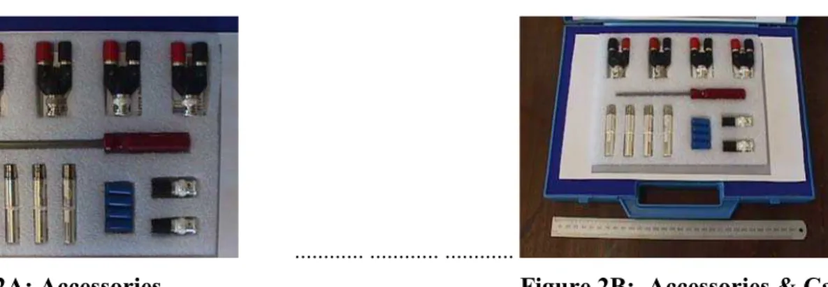
3.2 Accessories

The set of accessories accompanied the travelling standard were

:-• A 3 mm hex ball driver, for the 8 bolts that secure the red wooden box top to bottom • 4 off BNC - dual 4 mm adaptors

• 4 off BPO (MUSA) - BNC adaptors • 2 off BNC - single 4 mm adaptors

3.3 Transit cases

Special care was applied to the way in which the travelling standard was packed and trans-ported between laboratories. As the schedules were tight, air-freight was the only viable option.

During transit, the red wooden box was secured in a large ABS plastic case with padded foam inserts. This plastic case and the accessories case were in turn secured within a large aluminum transit case with padded foam inserts.

The transit system was tested at NPL sometime prior to the first scheduled visit : The alu-minum transit case was held approximately 1 m above a concrete pavement and dropped, with one corner of the case pointing towards the ground. Before-and-after measurements did not reveal any significant change to the measured parameters of the travelling standard. Shock detectors were mounted on the red wooden box, on the ABS case and the other transit case; only one of these detectors was activated throughtout the entire programme. Minor damage was observed during the comparsion to the outer transit case and repairs and addi-tions were made to the securing latches and hasps. No visible damage was seen or reported to the intermediate ABS case, the red wooden box or the travelling standard itself.

4 Measurements

Details of the tests, methods, defining conditions and related information were given in the Technical Procedure document in Appendix R.

5 Method of measurement used by each participant

5.1 Method of measurement used by CEM, Spain

The ratios 0.1 to 0.9 and 1/11 to 10/11 have been measured by the known "straddling" method with direct and reverse connections using a calibration transformer in taps 0.1 to 0.9 and 1/11 to 10/11.

(10)

The ratio 0.01 was measured using an auxiliary voltage ratio transformer whose deviation from its nominal value at ratio 0.1 is previously measured, with an input voltage of 1V. This previous measurement is carried out by the same method as above. The most outstanding elements that the measuring system incorporates are: triaxial connections between the IVD traveling standard and the calibration transformer; specially designed networks to detect current, to give potential to the intermediate screen, to adjust cross-capacitances in the lines and to provide injections in phase and quadrature to produce the main balance.

An RC network adjusted, jointly with the rest of the components in the line of quadrature injection, produces a precise 90º in advance at 1 kHz.

5.2 Method of measurement used by IEN, Italy

The measurements have been carried out with a new system for ac voltage ratio absolute calibration. The system is based on the simplest possible application of the bootstrap method [2–5]. The system is built around a new two-stage divider, having k: 10, k: 11 and 1: 100 ratios; a two-stage bootstrap transformer (1:10 and 1:11 ratios) with a guarded one-turn secondary 8 stage with adjustable cross-capacitances; two-secondaries (k:10 and k:11) transformer for easy guarding. The system does not involve injection/detection transformers, but is based on a direct measurement of the voltage differences with a purpose-built vector voltmeter [6]. During the step-up the voltage differences are read directly with the vector voltmeter which has an extremely high common-mode rejection ratio, exceeding 180 dB at 1 kHz. The vector voltmeter has the following properties:

1. completely guarded structure to achieve very high apparent input impedance;

2. an extremely high common-mode rejection ratio (CMRR), greater than 180 dB at 1 kHz

3. a programmable-gain amplification stage (full-scale dynamics are in the range 500 ~V to 500 n V)

4. a dual-channel synchronous demodulating stage with high harmonic rejection; 5. 8 battery operation

6. computer-controlled operation, via an optical fibre interface [7].

The method is insensitive to several possible systematic errors of the vector voltmeter or those coming from the bootstrap operation

5.3 Method of measurement used by KRISS, Korea

The AC voltage ratio calibration system of KRISS [8] has the following functions: - Ra-tio terminals: 0.01, 0.1 to 1.0, 0.01 to 0.1, and 1/11 to 10/11, - ResoluRa-tion for α and β : 10−10, Selfcalibration by comparison with the reference winding using triaxial cables,

-Adjustment function to minimize internal loading caused by distributed shunt impedances and leakage impedances in both the divider winding and the calibration system.

(11)

A modified method for consecutive comparison of a voltage difference on the taps of each section with a stable isolated reference voltage was used for calibration of the ratio trans-former. The reference voltage is formed by special tri-axial winding of the same transformer, so the used method is rather self-calibration than calibration. The creating of EMF in both ratio and reference winding by the same magnetic flux eliminates any nonlinear distortions between them which are fundamental restriction of accuracy in this method. The potentials of internal screens of tri-axial cables connecting to both the reference winding and a mea-sured section of the ratio winding, are driven by auxiliary sources. Any offset in the detector is eliminated by injection of a current in an additional winding of the detector transformer instead of balancing of currents in gaps of tri-axial cable.

5.4 Method of measurement used by LCIE, France

The divider CCEM-ACVRS01 was calibrated by comparison with a reference divider ESI type DT72A previously calibrated.

The comparison was carried out directly for all ratios by means of a General Radio zero de-tector and a voltage injection device adjusted in phase and quadrature. The voltage injection device is introduced in the detection arm of the bridge.

The determination of the ESI type DT72A divider linearity errors was performed as the following:

1. Direct comparison between the unknown divider ratio and the same ratio of a tare divider for all positions of the 1st, 2nd and 3rd decades.

2. Insertion of a voltage transformer (1) in the detection arm and comparison be-tween the unknown divider ratio and the tare divider ratio for the just inferior position for all positions of the 1st, 2nd and 3rd decades.

By combining all values of voltage injected (in phase and quadrature) to obtain the balance, it is possible to determine the linearity error of the unknown divider.

(1) Ratio 1:10 for the 151 decade, 1:100 for the 2nd decade and 1:1000 for the 3rd decade.

5.5 Method of measurement used by METAS, Switzerland

The n/10 and n/11 ratios of the CCEM-ACVRS01 Inductive Voltage Divider (UUT) were calibrated using the so-called "boot-strap" method [9, 10] either with or without the use of an auxiliary IVD.

When an auxiliary IVD(AUX) is used the measurement procedure is as follows. First, both dividers are compared with their outputs set at the same nominal value. An injection system ∆ En and a null detector is used to measure the voltage difference. Then, the UUT is set

one step higher and a supplementary step-injection system was introduced in the circuit. The injected voltage ∆ E’nneeded to null the detector is measured. Finally, the AUX is set

one step higher. Both IVD outputs are nominally equal again, so they can be compared 10

(12)

without the step- injection system. This procedure of increasing first the UUT and then the AUX can be repeated from the lowest to the highest ratio output of the IVD. The set of equations involving the measured values of ∆ En and ∆ E’n can be solved and the in-phase

and quadrature deviations from the nominal output ratios can be calculated for both dividers. In the case when all the ratio taps of the UUT are separately available, the auxiliary IVD is not needed any more and the ratio {n} of the UUT can be directly compared to the tap {n+1}. The number of steps needed to calibrate UUT is smaller than for the method using an auxiliary IVD.

The 1/100 ratio of the CCEM-ACVRS01 IVD was calibrated by comparison with our ref-erence 8-Dial IVD (PR1). In this case, the error of the output ratio of the UUT is directly determined by comparison to the same nominal output ratio of the reference IVD which has a known error.

5.6 Method of measurement used by NIM, China

The linear correction ∆ K_ΣL(K_N) of transfer ratio for the core of shielding plug of all indica-tions i/N (i=0~N, N=10 or 11) have determined by the Method "Comparison Method with Bidirectional (positive/negative) Reference Winding" [11], Design principle of the measure-ment method are following:

1. The reference voltage divider will provide the supporting voltage for the reference winding. Then the comparison between reference winding voltage and the sectional voltage of calibrated voltage divider could be processed under the practical working conditions of the calibrated voltage divider.

2. The Reference voltage of Reference Winding is defined as an increment of this winding voltage when connect of its original winding is changed without short to input voltage of the calibrated voltage divider. Based on cumulate principle this Reference voltage is irrelevant without the potential of low point by this Reference Winding, if its circuit parameters are linear.

3. For the linear correction ∆ K_ΣL(K_N) of transfer ratio two independent measurements will be taken by commutate the original winding. The average of two independent measurement results will be used as final result. The practical design of measurement process calculate that, most errors of the measurement equipment can be eliminated by the subtracting of the data pairs. Most of the remaining error factors will produce op-posite errors during the bidirection (positive/negative) process. So, besides providing the measurement result of linear corrections ∆ K_ΣL(K_N), this method can also provide the impersonal experimental base for evaluating the limit error (extended uncertainty) of the measurement result.

(13)

5.7 Method of measurement used by NIST, USA

Two methods were used to determine the errors of the IVD. With the exception of the 0.01 tap for which a “bootstrap” bridge was used, the bridge was based upon the step-up or “strad-dling” method. The IVDs were of a two-stage design with additional circuitry to perform triaxial guarding, coaxial equalization, Wagner isolation, auxiliary signal injection and phase sensitive detection. With this straddling method, a critical factor influencing bridge accuracy is the common mode rejection of the auxiliary IVD. The 1:1 ratio errors of the auxiliary IVD must remain constant irrespective of the common mode level to which it is driven. This requirement is addressed by vary careful design of guarded shields that enclose the auxiliary IVD.

5.8 Method of measurement used by NMI, Austraila

AC voltage ratio is measured at NMIA using a build-up technique based on the method described by Thompson [12]. The signal measurement system is described by Small and Leslie [13]. Further to Thompson’s original work, the build-up measurement system at NMIA has undergone considerable refinement and development. The main changes are: 1.Use of a bootstrap transformer separate from the transformer being calibrated to provide the isolated reference voltage. The shields of the purpose built bootstrap transformer are designed in such a way that the variation of output voltage with offset voltage is of the or-der of 1 nV/V and may be determined with small uncertainty (linear regression on multiple measurements sets was used to further reduce uncertainty). 2.Use of pre-excited (rather than single excitation) transformers, ensuring that output voltages are well defined and stable with respect to each other. 3.Core sense windings on the coaxial chokes and manually-adjusted injectors have been added where required. Note that each injection voltage is adjusted for every measurement. The uncertainty due to residual current imbalance has been determined experimentally to be negligible by testing the sensitivity of the measurement to the adjust-ment of the injectors. 4.The on/off switching of the calibrate signal is arranged so that the detector circuit impedance and the loading of the source remain unchanged. 5.A single wire connects the grounds of the bootstrap transformer and the ac voltage ratio standard. By coax-ial injection into its supply lead, the ground potentcoax-ial of the bootstrap transformer is adjusted for zero current in this wire, so that the grounds of the two transformers are equalised with-out causing unbalanced current flow in the coaxial conductors of the voltage comparator. The single wire is wrapped around the comparator circuit to minimise the area of the loop represented by the single wire and the outer conductors of the voltage comparator, thereby ensuring that the measurement is insensitive to coupling into this loop. The ratio of the 0.01 output voltage to the 0.1 output voltage was measured by comparison with a 10:1 inductive voltage divider previously calibrated by the build-up technique. From the build-up calibra-tion of the decade output voltage, the 0.01 ratio was then calculated.

(14)

5.9 Method of measurement used by NMI (ETL), Japan

Measurement method The traveling IVD was calibrated using a build-up method, the prin-ciple of which is based on the techniques developed by A. M. Thompson [12]. So-called "special connectors" were used in the measurements, by which output voltage of the IVD can be measured as the open circuit voltage at its port. The measurement equipment includ-ing the special connectors was fabricated and evaluated by ourselves [14, 15].

5.10 Method of measurement used by NMi - Van Swinden

Laboratorium, The Netherlands

A bootstrapping method [9] is used for calibrations of inductive voltage dividers (IVD) and voltage ratio transformers. In this comparison, the bootstrapping method was applied to mea-sure the n/10 and n/11 ratio taps of the (traveling) inductive voltage divider (IVD). The 0.01 output was measured by comparison with a calibrated IVD. For the bootstrapping method, the uncertainty in the ratio measurements is mainly determined by the contributions of the ratio difference measurements between the divider under test (traveling standard) and the auxiliary divider. The measurements are performed by null-detection on a phase sensitive detector. An injection system in series with the output of the auxiliary divider is used to balance the bridge.

5.11 Method of measurement used by NPL, UK

The NPL AC voltage ratio measurement system based on a bootstrapping method [2, 5]was used for the intercomparison measurements. The traveling inductive voltage divider (IVD) was compared against the NPL reference IVD, with both IVDs energised from a common AC voltage, with the voltage difference between their outputs being measured. The ratio errors of the traveling IVD were calculated from these measured differences and the known errors of the NPL reference IVD. This NPL reference IVD is maintained by measuring the difference voltage between adjacent taps.

5.12 Method of Measurement used by NPL, India

LF Impedance group of NPLI is having two standard IVDs. Each section of these IVDs is approachable through BPO connectors. Calibration of Standard IVD is done by absolute method using injection voltage technique. This setup was established in 1987 and reported in CPEM 88 [16]. This setup was improved to achieve an uncertainty of 1 to 2 parts in 109. Calibration of 8 decade IVDs is done by 1:1 comparison against standard IVD using injection voltage technique. The traveling standard was calibrated in this setup.

8 decade IVDs are used as reference standards for calibration of 6 and 7 decade IVDs re-ceived for calibration from industries and calibration laboratories [17–20].

(15)

5.13 Method of measurement used by NRC, Canada

The measurements of the CCEM-K7 comparison were made at 10 volts and 1 kHz using a modified straddle comparison bridge somewhat similar in basic design to that described in [5] (page 140). The major design differences include:

1. A coaxial straddle transformer with an internal 2-stage injection transformer on the central lead Triaxial connections between the straddle transformer, the triaxial detector and measured transformer.

2. Triaxial connections between the straddle transformer, the triaxial detector and mea-sured transformer.

3. Triaxial definition up to the BPO connectors, which attach to the measured trans-former.

4. A single detector (triaxial) on the central lead.

5. Measurements are only made with a single loop of the straddle transformer at one time, the other straddle transformer lead being left open.

6. Sensitivity of each single loop measurement is determined in situ.

Detector offsets were determined by reversal of the triaxial detector and measurement of the detector signal versus guard voltage of each single loop using a BPO Tee and with the straddle transformer driven with zero voltage. The successive ratios of the CCEM-K7 trans-former’s decade and elevenths taps were measured using the straddle transformer bridge. The linearized tap ratios were subsequently determined.

The 0.01 tap was measured by comparing a 1, 0.1, 0 transformer to the CCEM-K7 trans-former and then reducing the drive of the 1, 0.1, 0 transtrans-former by 10 and comparing to the CCEM-K7 0.1, 0.01, and 0 taps. An estimate of the voltage coefficient of the transformer is included in the uncertainty budget.

A single loop measurement consists of 25 measurements, each in a lockin amplifier time constant of 300 mS and at a range corresponding to ~1.5x10−6 of full scale (10V).

An additional 25 measurements with 1x10−6 injected into the central lead was used to

deter-mine the detector sensitivity which varies slightly for each loop. These are repeated for each of the two leads.

The reported results are the average of several complete straddle measurement sets.

5.14 Method of measurement used by PTB, Germany

The principle of the calibration is the well-known "bootstrap"-method. The constant output voltage of a reference transformer is compared in i steps (e.g. i = 10 for decade dividers with 10 winding groups) with the unknown output voltages of each winding group of the inductive voltage divider (device under test). The complex voltage differences, relative to the input voltage, are measured using a lock-in amplifier. From these readings the in-phase and quadrature voltage ratios as well as the uncertainties are then calculated using the software "GUM Workbench" (Version 1.2.11.56 Win32, see www.metrodata.de).

(16)

In Appendix N the calculation of the in-phase voltage ratio and the corresponding uncertainty at the nominal value 0.6 is shown as an example. The 10 in-phase readings α₁to α₁₀ of the difference voltages are added and divided by (-10) to receive the in-phase correction K_wR of the reference transformer. The corrections K_wt1to K_wt6 of each winding group can then be calculated by adding the in-phase correction K_wRof the reference transformer to the in-phase readings α₁to α₆. Summing up the in-phase corrections of every winding group K_wt₁to K_wt6 will result in the in-phase correction K_w6of the voltage ratio 0.6. The final result ipvr6 is the sum of the nominal value of Port 6 (= 0.6) and the in-phase correction K_w6.

5.15 Method of measurement used by SP, Sweden

The travelling Inductive Voltage Divider CCEM-ACVRS01 was calibrated by comparison with SPs primary inductive voltage divider in an inductive voltage divider comparison bridge. The comparison bridge consists of a two-staged primary inductive voltage divider and a R-C circuit for balancing the quadrature voltage difference between the primary standard and the inductive voltage divider under test. The in-phase voltage ratios and the quadrature voltage ratios for the primary inductive voltage divider were calibrated by comparison with a two-staged inductive voltage divider of the same construction with the in-phase voltage ratios and the quadrature voltage ratios determined at SP by a capacitance permutation method in a ca-pacitance bridge. The permutation method is based on five 100 pF and two 50 pF caca-pacitance standards of very high short term stability. The capacitance standards are compared with 1: 1 ratio measurements. Then, by measurements with different capacitance combinations, are the ratio corrections determined for the capacitance bridge inductive voltage divider. One 1000 pF and one 10 pF capacitance standard which are measured in a 1:10 ratio against the 100 pF reference is used for the determination of the 1:100 ratio corrections.

5.16 Method of measurement used by UME, Turkey

An AC voltage ratio measurement system was used for the intercomparison measurements. This system is a homemade and primary measurement system based on Bootstrapping method [9]. n/10 and n/11 reference two-stage transformers were used to compare two adjacent out-puts of n/10 and n/11 at travelling standard. In order to calibrate 1/100 ratio, a reference two-stage 1/100 transformer and a two-decade reference IVD were used. Second decade of the reference IVD was calibrated with 1/100 two-stage transformer based on Bootstrapping method. Real and imaginer errors of 1/100 two-stage transformer were calculated by using the calibration values of the reference IVD then 1/100 ratios of the travelling standard and 1/100 two-stage transformer were compared. Phase calibration of injection network was per-formed by using a 100 pF Fused-Silica standard capacitor and a 100 Ω Vishay resistor [5]. Injection transformers were calibrated with a reference 7-decade IVD [21].

(17)

5.17 Method of measurement used by VNIIM, Russia

Self-calibration method using a calibration transformer with a single output voltage ("boot-strap" method) is applied. It is analogous to the method [9] but has the following improve-ments:

1. additional winding of self-calibrated two-stage transformer is used instead of the external calibration transformer;

2. this additional winding is provided with double shielding; 3. conductor-pair coaxial design is used for the whole circuit;

4. special injection circuit is used for "zeroing" of an detector, to eliminate the currents (due to nonbalanced cross capacitance) that flow through detector and give incorrect balances;

5. self-calibrating transformer is supplied with two inputs - for 100 and 110 turns - for both magnetizing and ratio windings.

(18)

6 Results

6.1 Handling & treatment

Every participating laboratory sent a report to the Pilot Laboratory detailing the test method used to obtain the results and uncertainty budgets, in accordance with ISO “Guide to Uncer-tainty in Measurements” guidelines, referred to as the GUM model. [22]

6.2 Statistical analysis

Details of the statistical analysis can be found in Part 2 of the report.

References

[1] J. Fiander and G. Small, “An inductive voltage divider for international comparisons,” in Conference Digest CPEM 2000, pp. 224–225, 2000.

[2] J. Hill and T. Deacon, “Voltage-ratio measurement with a precision of parts in 109 and performance of inductive voltage dividers,” IEEE Trans. Instrum. Meas., vol. 17, pp. 269–278, 1968.

[3] K. Grohmann, “A step-up method for calibrating inductive voltage dividers up to 1 MHz,” IEEE Trans. Instrum. Meas., vol. 25, pp. 516–518, 1976.

[4] K. Grohmann, “An international comparison of inductive voltage divider calibration methods between 10 kHz and 100 kHz,” Metrologia, vol. 15, pp. 69–75, 1979.

[5] B. Kibble and G. Rayner, “Coaxial AC Bridges,” Report CEM 16, 1984.

[6] L. Callegaro, P. Capra, and A. Sosso, “Guarded vector voltmeter for ac ratio stndard calibration,” IMTC, vol. 3, pp. 1441–1444, 2001.

[7] L. Callegaro, P. Capra, and A. Sosso, “Optical fibre interface for distributed measure-ment and control in metrology set-ups: application to current sensing with fA resolu-tion,” IEEE Trans. Instrum. Meas., vol. 50, pp. 1634–1637, 2001.

[8] R. Lee, H. Kim, and Y. P. Semenov, “Ratio transformer and its calibration,” in Confer-ence Digest CPEM 2004, pp. 378–379, 2004.

[9] W. Sze, “An injection method for self-calibration of inductive voltage divders,” J. Res. Nat Bur. Stand, vol. 72C, no. 1, pp. 49–59, 1968.

[10] D. Homan and T. Zapf, “Two stage guarded inductive voltage divider for use at 100 kHz,” ISA Trans, vol. 9, pp. 201–209, 1970.

[11] H. Xiaobing, H. Xiaoding, L. Lingxiang, L. Jidong, and Q. Zhongtai, “Absolute mea-surement of the linear corrections for inductive voltage dividers by method "Compari-son method with reference winding.” Chinese reference.

(19)

[12] A. Thompson, “Precise calibration of ratio transformers,” IEEE Trans. Instrum. Meas., vol. 32, pp. 47–50, 1983.

[13] G. W. Small and K. E. Leslie, “Synthesising signal generator for use with lock-in ampli-fiers in audio frequency measurements,” IEEE Trans. Instrum. Meas., vol. 35, pp. 249– 255, 1986.

[14] Y. N. et al., “10:1 ratio transformer for capacitance measurement,” in Conference Digest CPEM 1996, pp. 364–365, 1996.

[15] Y. N. et al., “Calbration of 10:1 ratio transformer using Thompson’s method,” Metrolo-gia, pp. 353–355, 1997.

[16] A. Saxena, R. Dhar, S. Dahake, and K. Chandra., “Development of injection voltage technique for absolute calibration of inductive voltage divider at the National Physical Loboratory, India,” in Conference Digest CPEM 1988, 1988.

[17] A. Saxena, R. Dhar, S. Dahake, and K. Chandra, “Design and fabrication of 4 and 6 decade inductive voltage dividers,” Instrument Society of India, vol. 14, no. 2, pp. 117– 125, 1984.

[18] A. Saxena, N. Singh, R. Dhar, S. Dahake, and K. Chandra, “Design and development of precision 8 decade inductive voltage divider,” Research and Industry, vol. 32, pp. 1–4, 1987.

[19] S. Dahake, A. Saxena, and M. Saleem, “Absolute calibration of transformer ratio by straddling method,” Institution of Engineers, India, vol. 75, pp. 166–168, 1995.

[20] A. Saxena and M. Saleem, “A simple automatic system for calibration of inductive voltage dividers,” in Conference Digest CPEM 1996, p. 426, 1996.

[21] “Calibration certificate of reference 7 decade inductive voltage divider,” 2002. EKA.071 24.10.2002.

[22] International Organsiation for Standization, Geneva, Guide to the expression of uncer-tainty in measurement, 2 ed., 1995.

(20)

7 Appendix

Uncertainty Budgets

and

(21)

(22)

Appendix - A - Uncertainty Budget for CEM, Spain

Ratios 0.1 to 0.9

The real ratio of the output n of the IVD is : (n/10) +E(n), for n = 1 to 9. We calculate E(n) by the expression:

E(n) = (n/10) [0.9 à1 + 0.8 à 2 + .. + 0.1 à9 –((n-1)/n)à1 -((n-2)/n) à2- ((n-3)/n)à3-...(1/n)à n-1]

in which `a n is obtained according to Kibble and Rayner (Coaxial AC Bridges)

In CEM system, the `a n values are obtained from the following expressions:

`an(phase) = 10 r0 (r1p – r2p + r´1p – r´2p) / R

`_a_n_(quad)_{= 10 r}₀_{( r}_1q_{– r}_2q_{+ r´}_1q_{– r´}_2q_{) / R. R}_RC

being r, R y RRC parameters that result of auxiliary IVD readings use to balance and

transformer injections.

Table 1 and Table 2 include, as an example, the uncertainty budget of `an (phase) and `an (quad)

respectively, for positions of measurement n = 1 and n = 2.

Ratios 1/11 to 10/11

The real ratio of the output n of the IVD is : (n/11) +E(n), for n = 1 to 10. We calculate E(n) by the expression:

E(n) = (n/11) [(10/11)à1 + (9/11)à 2 +...+ (1/11)à 1 – ((n-1)/n)à 1 -((n-2)/n)à 2 - ((n-3)/n)à 3 -...- (1/n)à n-1]

In this case the `an values are obtained in a similar way as before. Ratios 0.01

The real ratio of the output of the IVD is : 0,01 + E(0.01). This E(0.01) deviation is obtained from

the deviation of 0.1 ratio of an auxiliary transformer (input 1 V), and of the deviation of 0.1 ratio of the IVD travelling standard (input 10 V) previously measured.

(25)

(26)

Appendix - B -1

Appendix - B - Uncertainty Budget for NMI, Australia ( formally CSIRO)

The following sources of uncertainty were considered:

Type A:

Each ratio was measured on at least three separate occasions. The mean value of the measured ratios is reported, and a Type A uncertainty calculated.

Type B:

Reference uncertainty. AC voltage ratio is realised directly at NML and, as

such, does not depend on references calibrated at NML or by another laboratory.

Linearity of detector system. The linearity of the detector system (including

the lock-in amplifier) was measured and found to be better than 1 in 105 of the measured signal (no deviations from linearity could be detected to this level). The measured signal is, in all cases, at least 1x10-6 of the input voltage, V. We are confident therefore that the uncertainty from this source is less than

V -11

10

1× . Assuming a square law distribution with a semi-range of

V -11

10 5 .

0 × , we estimate the standard uncertainty as ₀_.₂₉×₁₀-10V_{with 50}

degrees of freedom.

Definition of calibrate signal. The calibrate signal of _1×₁₀-6V _{is derived}

from two cascaded 1000:1 separately-excited ratio transformers whose ratio errors are not expected to be greater than 1 in 105. We assume that the ratio error for each 1000:1 transformer is zero, and take the uncertainty in the error as 1x10-5 of the applied voltage, treated as a square law distribution. We therefore take the uncertainty in the calibrate signal as ₁_.₁₅×₁₀-11V_.

The uncertainty in the measured errors of the IVD under test depend on the uncertainty in the calibrate signal in a complex way, but provided the

measured errors are no greater than the calibrate signal then the uncertainty in the measured errors of the IVD under test will be no greater than the

uncertainty in the calibrate signal. We expect therefore that the uncertainty from this source is less than 1.15x10-11 of input voltage with infinite degrees of freedom.

Temperature. Variations in the ratio errors with variations in temperature are accounted for in the Type A assessment. Any uncertainty in the ratio error associated with the uncertainty in the temperature measurement is assumed to be negligible.

Magnetization of artefact. The IVD was demagnetized at the outset and again at the conclusion of the calibration. There was no evidence of acquired residual magnetization on either occasion. We assume therefore that any uncertainty in the ratio errors due to magnetization of the artefact is negligible.

Frequency. Ratio errors at 55 Hz were found to be strongly frequency dependent. Ratio errors measured at 55.0 Hz differed from those measured at

(27)

Appendix - B -2

55.1 Hz by typically 2 in 109 of input voltage. Since our realisation of frequency is many orders of magnitude better than 0.1 Hz, we believe it is unlikely that this source of uncertainty is significant. However, no attempt has been made to accurately determine the frequency dependence of the ratio errors or to include frequency dependence as a source of uncertainty.

Excitation level. The input voltage was measured with a calibrated, 5½ digit multimeter. No attempt has been made to accurately determine the

dependence of the ratio errors on excitation level or to include excitation level as a source of uncertainty.

Resolution. The resolution of the system is ±_1×₁₀-11V_{. Treated as a square}

law distribution, the resolution uncertainty is therefore ₀_.₅₈×₁₀-11V_with

infinite degrees of freedom.

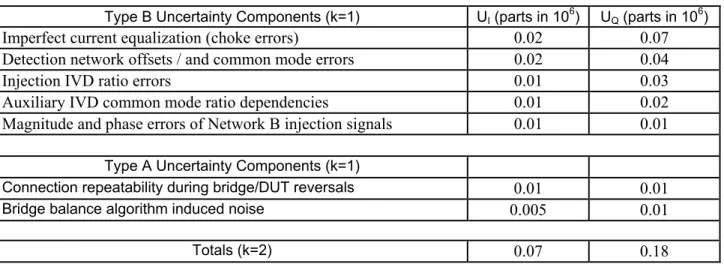
Summary of uncertainties: Source Assessed as: Standard Uncertainty Degrees of Freedom Repeatability Type A (1 – 44) x10-10 2-7 Linearity of detector system Type B 0.03 x10-10 50 Definition of calibrate signal Type B 0.12 x10-10 Infinite Resolution Type B 0.06 x10-10 Infinite

(28)

(29)

L. Callegaro, V. D’Elia: Partecipation of IEN to CCEM-K7. July 2003.

6

IV. MEASUREMENTS

The travelling standard [10] has a tap configuration different from Fig. 2, since the standard is constructed to provide at the same time k/10, k/11 and 1/100 ratios. In particular,

- all connectors are BPO MUSA instead of triax;

- the magnetizing 0, 100 and 110 taps are a single BPO connector;

- the feeding 0, 100 and 110 taps are a single connector called input;

- the output 0, 0.1, 0.2, ... 0.9, 1.0 taps are splitted in two sets of taps called 0, 1/10, ... 9/10 and 1/11, 2/11, ... 10/11;

- the output 0.01 is called 1/100;

- the output 0 is not shorted, since the voltage output is defined in a non-coaxial way as the voltage between tap k and tap 0.

Calibration of k/10 and k/11 taps

Apart from these differences, the circuit employed is the same of Fig. 2 and the procedure for calibration of k/10 and k/11 taps is similarly carried out.

Calibration of 1/100 tap

The calibration of 1/100 tap is carried out by comparison of the taps 1/10, 1/100 and 0 of the travelling standard against the taps 1, 1/10 and 0 of an auxiliary IVD1, in turn calibrated with the circuit of Fig. 2 and energized with an auxiliary 10:1 IVD2. IVD1 is calibrated using the bootstrap technique; IVD2 ratio errors don’t enter the calibration of 1/100 tap.

V. UNCERTAINTY EVALUATION

The uncertainty in the estimation of the ratio errors

{ }

r_k can be computed from the

uncertainty in the estimation of the set

{ }

e_k using Eqn. 3. Assuming that measurement errors given by :

- limited resolution of the measurement device (voltmeter reading); - uncertainty of V_in;

- effects of temperature coefficients of the system within the temperature range

considered (23±0.5 °C);

- effects of humidity coefficients of the system within the humidity range considered

(50±10 RH)

- effects of frequency coefficient of the standard measured within the frequency range

considered (997-1003 Hz); are negligible,

(30)

L. Callegaro, V. D’Elia: Partecipation of IEN to CCEM-K7. July 2003. 7

(

k

)

(

k k k

)

k k g e c E o e = 1+ ⋅ * + +∆ + (4) where * k

e is the true value of e ;_k

k

e is the voltage reading;

k

g is the complex gain error of the measurement. Takes into account the

residual gain error of the voltmeter after the calibration procedure, residual loadings on the voltage taps;

k

c is the complex common-mode error. Takes into account the limited

common-mode rejection ratio of the voltmeter

k

E

∆ is the variation of E because of imperfect or unequalized guarding,

causing loading of MIVD, in the measurement arm. Takes also into account guard currents in BT;

k

o is the measurement complex offset. Takes into account the electronic

voltage offset of the voltmeter, and interferences due to stray magnetic fields from the magnetic devices.

Reasonable assumptions: g

g_k = . Short-term constancy of the gain error during the measurement cycle; o

o_k = . Short-term constancy of the offset during the measurement cycle. It assumes that

the electronics is stable during the measurement period, and that possible interference effects due to stray magnetic fields from the magnetic devices (each one carrying constant flux during the entire measurement) are constant;

(

k n

)

c

c_k = ⋅ / . The common-mode error is considered proportional to the corresponding

common-mode voltage, in turn proportional to the tap index. This is the standard assumption for CM error in electronic amplifiers.

(

k n

)

E

E_k =∆ ⋅ /

∆ . E deviation proportionality to unequalized guard currents or loading

effects, in turn proportional to the corresponding common-mode voltage.

(31)

L. Callegaro, V. D’Elia: Partecipation of IEN to CCEM-K7. July 2003. 8

(

)

(

c E

)

o n k e g e_k _k +      ∆ + + ⋅ + = 1 * (5) Recalling Eqn. 3: in n i i k i i k V e n k e r

∑

= = − = 1 1 ) (6) by direct substitution,

(

)

(

)

(

and its maximum absolute value is p(k/2) =n/8 .

In conclusion, a constant offset error has no effect on r ; both the gain error g and the_k relative CM errors c /V_inand∆E /V_in have, for n=10 or n=11, sensitivity coefficients for the propagation of uncertainty of e to _k r , close to unity._k

Estimation of the gain error g

The gain error results from calibration errors of the voltmeter and drifts after calibration. We estimate a gain error

0 =

g +j0; )u(g = 0.01, Gaussian

Estimation of the common-mode error c

Testing the voltmeter for common-mode rejection showed no appreciable common-mode effects within the noise of the voltmeter. Thus we put the uncertainty for cequal to the rms noise of the voltmeter

c= 0+j0 V; u(c)= 10 nV , Gaussian Estimation of the voltage error E∆

This is the most difficult error to ascertain. We put

4 10−9V_in ⋅ = ∆ , Gaussian

(33)

10 Evaluation of sensitivity coefficients

By differentiation, and computing at point

[

g=0,c=0,∆E=0

]

:

( )

* k k r r s = (11)

( )

= _ − _ n n k k V c s in 2 ) ( 1 (12)

(

∆

)

= _ − _ n n k k V E s in 2 ) ( 1 (13) Standard uncertainty

The estimation of the standard uncertainty of ratio error is considered as the quadratic sum of type B uncertainty (estimated as above) and type A uncertainty, estimated as the experimental standard deviation of several measurement cycles (more than 10). The expanded uncertainty has been evaluated considering infinite degrees of freedom for type B uncertainty, and for a 95% confidence interval, by calculating the equivalent degrees of freedom with the Welch-Satterthwaite formula.

1/100 tap

A straightforward evaluation of uncertainty for 1/100 tap require a complex analysis since many passages are involved. For simplicity, we make a simplified evaluation with the same expressions of k/10 and k/11 taps, but expanding the instrumental uncertainty.

VI. RESULTS

The calibration results, and standard and expanded uncertainties, are reported in Tab. 1.

VII. CONCLUSIONS

We developed at IEN an implementation of the well-known bootstrap techinque for the calibration of ac voltage ratio standards. The implementation is simple, and quick to operate, thanks to the use of a special vector voltmeter, to permit direct reading of voltage differences. A guarded network comprising a bootstrap transformer and a guard divider, permits to calibrate k/10, k/11 and 1/100 taps of a two-stage divider, which in turn will be used (with a similar network using the same components) to calibrate customers’ dividers. Construction details, examples of calibration and notes about uncertainty are given.

(34)

(35)

Appendix - D - Uncertainty Budget for KRISS, Korea

UNCERTAINTY BUDGET FOR RATIO OF 0.01 (KRISS

)

In-phase Quadrature

No Cause of uncertainty Type Standard

uncertainty Accuracy of uncer. estimate (%) Calculated degree of freedom Standard uncertainty Accuracy of uncer. estimate (%) Calculated degree of freedom 1 2 3 4 5 6

Adjustment of injection circuits Zero balance of detector transformer Potential difference among outer

conductor of BPO connectors Magnetic field effect on reference

voltage circuit

Leakage capacitance through screen of coaxial cable Repeatability of measurements B B B B B A 9 10 4 -´ 9 10 4 -´ 9 10 4 -´ 9 10 4 -´ 9 10 4 -´ 9 10 4 -´ 30 30 30 30 30 6 6 6 6 6 14 9 10 5 -´ 9 10 5 -´ 9 10 5 -´ 9 10 5 -´ 9 10 5 -´ 9 10 10 -´ 30 30 30 30 30 6 6 6 6 6 14 Combined standard uncertainty

Expanded uncertainty

Effective degrees of freedom Coverage factor 9 10 80 . 9 -´ 8 10 0 . 2 -´ 37 2.03 8 10 5 . 1 -´ 8 10 0 . 3 -´ 40 2.02 Appendix - D - 1

(36)

UNCERTAINTY BUDGET FOR RATIO FROM 0.1 TO 0.9 (KRISS)

In-phase Quadrature

voltage circuit

(37)

UNCERTAINTY BUDGET FOR RATIO FROM 1/11 TO 10/11 (KRISS)

In-phase Quadrature

voltage circuit

(38)

(39)

Appendix - E - Uncertainty Budget for LCIE, France

For ratios 1/10, 2/10, 3/10, 4/10, 5/10, 6/10, 7/10, 8/10 and 9/10 : From the equation 1 ,

) ( ) ( ). 1 .( 2 ) (N_x N_n N_n2 u2 K u2 1_n u ₌ _- ₊ ₊ e

With u(K)=u(K_inj)=u(K_inj₀)=u(K_inj₁) and u absolute uncertainties. For ratios 1/100 and 1/11 :

From the equation 2 ,

) ( ). ) . 10 ( 1 .( 2 ) ( ) ( . ) . 10 ( ) (N N 2u2 ₁1 u2 2 N N 2 N 2 u2 K u x = n e + en + - n + n + n

With u(K)=u(K_inj)=u(K_inj₀)=u(K_inj₁) and u absolute uncertainties. For ratios 2/11, 3/11, 4/11, 5/11, 6/11, 7/11, 8/11, 9/11 and 10/11 : From the equation 3 ,

) ( ) ( ). 1 .( 2 ) (N N N 2 u2 K u2 e u _x = - _n + _n +

With u(K)₌u(K_inj)₌u(K_inj₀)₌u(K_inj₁)and u absolute uncertainties.

(40)

Uncertainty components (phase)

Component Ratio Standard uncertainty value Probability distribution/ method of evaluation Sensitivity

coefficient Uncertainty contribution

Degrees of freedom Reference divider (linearity error) 1/100 1/10 2/10 3/10 4/10 5/10 6/10 7/10 8/10 9/10 1/11 2/11 3/11 4/11 5/11 6/11 7/11 8/11 9/11 10/11 1,1.10-8 1,1.10-8 1,9.10-8 2,5.10-8 2,8.10-8 2,9.10-8 2,8.10-8 2,5.10-8 1,9.10-8 1,1.10-8 1,1.10-8 1,9.10-8 2,5.10-8 2,8.10-8 2,9.10-8 2,9.10-8 2,8.10-8 2,5.10-8 1,9.10-8 1,1.10-8 Normal/B 1 1,1.10-8 1,1.10-8 1,9.10-8 2,5.10-8 2,8.10-8 2,9.10-8 2,8.10-8 2,5.10-8 1,9.10-8 1,1.10-8 1,1.10-8 1,9.10-8 2,5.10-8 2,8.10-8 2,9.10-8 2,9.10-8 2,8.10-8 2,5.10-8 1,9.10-8 1,1.10-8 500 500 500 500 500 500 500 500 500 500 500 500 500 500 500 500 500 500 500 500 Temperature effect All 0,2.10 -8 ArcSinus/B 1 0,2.10-8 500 Compensati on voltage effect All 1,8.10-8 Rectangular/B 2.(1-N +_n N_n2) 2.(1-N +_n N_n2).1,8.10-8 500 Detector stability All 0,2.10 -8 Rectangular/B 2.(1-N +_n N_n2) 2.(1-N +n Nn2).0,2.10 -8 500 Upstream decades effect 1/100 1/10 2/10 3/10 4/10 5/10 6/10 7/10 8/10 9/10 1/11 2/11 3/11 4/11 5/11 6/11 7/11 8/11 9/11 10/11 0 0 0 0 0 0 0 0 0 0 0 6,0.10-8 6,0.10-8 6,0.10-8 6,0.10-8 6,0.10-8 6,0.10-8 6,0.10-8 6,0.10-8 6,0.10-8 Rectangular/B 1 0 0 0 0 0 0 0 0 0 0 0 1,8.10-8 1,8.10-8 1,8.10-8 1,8.10-8 1,8.10-8 1,8.10-8 1,8.10-8 1,8.10-8 1,8.10-8 500 500 500 500 500 500 500 500 500 500 500 500 500 500 500 500 500 500 500 500 Appendix - E-2

(41)

Ratio Combined uncertainty (2s) 1/100 1/10 2/10 3/10 4/10 5/10 6/10 7/10 8/10 9/10 1/11 2/11 3/11 4/11 5/11 6/11 7/11 8/11 9/11 10/11 1,1.10-8 2,6.10-8 2,9.10-8 3,3.10-8 3,5.10-8 3,6.10-8 3,5.10-8 3,3.10-8 2,9.10-8 2,6.10-8 3,5.10-8 3,4.10-8 3,7.10-8 3,9.10-8 4,0.10-8 4,0.10-8 3,9.10-8 3,7.10-8 3,4.10-8 3,1.10-8 Appendix - E-3

(42)

Uncertainties components (quadrature) Component Ratio Standard uncertainty value Probability distribution/ method of evaluation Sensitivity

coefficient Uncertainty contribution

Degrees of freedom Reference divider (linearity error) 1/100 1/10 2/10 3/10 4/10 5/10 6/10 7/10 8/10 9/10 1/11 2/11 3/11 4/11 5/11 6/11 7/11 8/11 9/11 10/11 1,1.10-8 1,1.10-8 1,9.10-8 2,5.10-8 2,8.10-8 2,9.10-8 2,8.10-8 2,5.10-8 1,9.10-8 1,1.10-8 1,1.10-8 1,9.10-8 2,5.10-8 2,8.10-8 2,9.10-8 2,9.10-8 2,8.10-8 2,5.10-8 1,9.10-8 1,1.10-8 Normal/B 1 1,1.10-8 1,1.10-8 1,9.10-8 2,5.10-8 2,8.10-8 2,9.10-8 2,8.10-8 2,5.10-8 1,9.10-8 1,1.10-8 1,1.10-8 1,9.10-8 2,5.10-8 2,8.10-8 2,9.10-8 2,9.10-8 2,8.10-8 2,5.10-8 1,9.10-8 1,1.10-8 500 500 500 500 500 500 500 500 500 500 500 500 500 500 500 500 500 500 500 500 Temperature effect All 0,2.10 -8 ArcSinus/B 1 0,2.10-8 500 Compensati on voltage effect All 1,8.10-8 Rectangular/B 2.(1-N +_n N_n2) 2.(1-N +n Nn2).1,8.10 -8 500 Detector stability All 0,2.10 -8 Rectangular/B 2.(1-N +_n N_n2) 2.(1-N +_n N_n2).0,2.10-8 500 Upstream decades effect 1/100 1/10 2/10 3/10 4/10 5/10 6/10 7/10 8/10 9/10 1/11 2/11 3/11 4/11 5/11 6/11 7/11 8/11 9/11 10/11 0 0 0 0 0 0 0 0 0 0 0 240.10-8 240.10-8 240.10-8 240.10-8 240.10-8 240.10-8 240.10-8 240.10-8 240.10-8 Rectangular/B 1 0 0 0 0 0 0 0 0 0 0 0 69.10-8 69.10-8 69.10-8 69.10-8 69.10-8 69.10-8 69.10-8 69.10-8 69.10-8 500 500 500 500 500 500 500 500 500 500 500 500 500 500 500 500 500 500 500 500 Appendix - E-4

(43)

Ratio Combined uncertainty (2s) 1/100 1/10 2/10 3/10 4/10 5/10 6/10 7/10 8/10 9/10 1/11 2/11 3/11 4/11 5/11 6/11 7/11 8/11 9/11 10/11 1,1.10-8 2,6.10-8 2,9.10-8 3,3.10-8 3,5.10-8 3,6.10-8 3,5.10-8 3,3.10-8 2,9.10-8 2,6.10-8 3,5.10-8 69.10-8 69.10-8 69.10-8 69.10-8 69.10-8 69.10-8 69.10-8 69.10-8 69.10-8 Appendix - E-5

(44)

(45)

Appendix - F - 1

Appendix - F - Uncertainty Budget for METAS, Switzerland

Tables below give the detailed uncertainty budget for the ratios 1/100 and n/10 measured at 10 V, 1000 Hz.

in-phase ratio

Uncertainty components (10-8) type 1/10 2/10 3/10 4/10 5/10 6/10 7/10 8/10 9/10 n

reproducibility of ratio measurements A 0.2 0.3 0.3 0.4 0.5 0.9 1.2 1.3 1.1 12 injection accuracy and linearity B 0.3 0.3 0.3 0.3 0.3 0.3 0.3 0.3 0.3 8 offset of the comparator bridge B 0.5 0.5 0.5 0.5 0.5 0.5 0.5 0.5 0.5 50 offset of the step-transformer B 0.4 0.7 1.0 1.1 1.2 1.1 1.0 0.7 0.4 8

load of the IVD B 0.3 0.4 0.4 0.3 0.2 0.3 0.4 0.4 0.3 50

combined standard uncertainty 1σ 0.8 1.1 1.2 1.3 1.4 1.6 1.7 1.6 1.3

effective degrees of freedom 64 32 21 17 17 25 29 27 26

coverage factor 2.1 2.1 2.1 2.2 2.2 2.1 2.1 2.1 2.1

expanded uncertainty (95.45%) 1.6 2.2 2.6 2.9 3.0 3.3 3.5 3.5 2.7

quadrature ratio

Uncertainty components (10-8) type 1/10 2/10 3/10 4/10 5/10 6/10 7/10 8/10 9/10 n

reproducibility of ratio measurements A 0.4 0.6 0.8 0.8 0.7 0.6 0.5 0.3 0.2 12 injection accuracy and linearity B 0.6 0.6 0.6 0.6 0.6 0.6 0.6 0.6 0.6 8 offset of the comparator bridge B 0.5 0.5 0.5 0.5 0.5 0.5 0.5 0.5 0.5 50 offset of the step-transformer B 2.1 3.7 4.8 5.5 5.8 5.5 4.8 3.7 2.1 8

load of the IVD B 2.6 3.8 3.9 3.2 2.0 3.2 3.9 3.8 2.6 50

combined standard uncertainty 1σ 3.5 5.4 6.3 6.5 6.2 6.5 6.3 5.4 3.5

effective degrees of freedom 44 31 22 15 11 15 21 31 43

coverage factor 2.1 2.1 2.1 2.2 2.3 2.2 2.1 2.1 2.1

expanded uncertainty (95.45%) 7.1 11.3 13.4 14.2 14.1 14.2 13.4 11.3 7.1

1/100 ratio

Uncertainty components (10-8) type in-phase quadrature n reproducibility of ratio measurements A 1.3 2.2 3

injection accuracy and linearity B 0.3 0.6 8

offset of the comparator bridge B 0.5 0.5 50

uncertainty on the reference B 3.0 3.5 50

combined standard uncertainty 1σ 3.3 4.2

effective degrees of freedom 47 29

coverage factor 2.1 2.1

Key comparison CCEM-K7: AC voltage ratio

NRC Publications Archive

Archives des publications du CNRC

Key Comparison CCEM-K7 :

AC Voltage Ratio

Draft B Report - Version I - Part 1

May 20, 2011

Contents

List of Tables

1 Introduction

2 Organisation

2.1 Organisation

2.2 Participants

2.3 Testing Schedule

3 Calibration Artefact & Shipping

3.1 The Travelling Standard

3.2 Accessories

3.3 Transit cases

4 Measurements

5 Method of measurement used by each participant

5.1 Method of measurement used by CEM, Spain

5.2 Method of measurement used by IEN, Italy

5.3 Method of measurement used by KRISS, Korea

5.4 Method of measurement used by LCIE, France

5.5 Method of measurement used by METAS, Switzerland

5.6 Method of measurement used by NIM, China

5.7 Method of measurement used by NIST, USA

5.8 Method of measurement used by NMI, Austraila

5.9 Method of measurement used by NMI (ETL), Japan

5.10 Method of measurement used by NMi - Van Swinden

Laboratorium, The Netherlands

5.11 Method of measurement used by NPL, UK

5.12 Method of Measurement used by NPL, India

5.13 Method of measurement used by NRC, Canada

5.14 Method of measurement used by PTB, Germany

5.15 Method of measurement used by SP, Sweden

5.16 Method of measurement used by UME, Turkey

5.17 Method of measurement used by VNIIM, Russia

6 Results

6.1 Handling & treatment

6.2 Statistical analysis

References

7 Appendix

Uncertainty Budgets

and

Table 1:

`a

and

`a

phase values uncertainty budget

Table 2:

`a

and

`a

quadrature values uncertainty budget

{ }

{ }

(

)

(

)

(

)

(

)

(

)

(

)

∑

∑

(

)

(

)

(

)

∑

∑

∑