The Wealth-Health Nexus: New Global Evidence

The Wealth-Health Nexus: New Global Evidence

Vishal Chandr Jaunky

Published online: 14 November 2012

# International Atlantic Economic Society 2012

Abstract Using a world sample of countries, this paper re-examines the U-shaped relationship between per capita GDP (wealth) and life expectancy at birth (health). Since cross-sectional dependence across countries is detected, second-generation panel unit root and cointegration tests are employed. All the variables are found to be integrated in one order as well as cointegrated. Various quadratic specifications are also employed and the hypothesis is confirmed.

Keywords Per capita GDP . Life expectancy . Cross-sectional dependence . Panel FMOLS

JEL I15 . C33 . O11

Introduction

Healthcare improvements constitute a major moral prerogative to any nation. Healthy citizens, whether unskilled or skilled, enhance an economy’s productive capacity by being both physically and mentally apt. As such, the question of whether better health care can stimulate economic growth intrinsically arises. There is an on-going debate in literature on the impact of increased life expectancy on the wealth of nations and diverse results have been obtained.

Cervellati and Sunde (2011) theorized a non-monotonic connection between life expectancy and economic growth,“… in which the demographic transition repre-sents an important turning point for population dynamics and hence plays a central DOI 10.1007/s11293-012-9347-x

I would like to express my sincere thanks to Thomas F. Rutherford and Massimo Filippini, John Virgo and

an anonymous referee for their comments on an earlier version of this paper. Errors, if any, are the author’s

own only.

V. C. Jaunky (*)

Centre for Energy Policy and Economics, ETH Zurich, Zurichbergstrasse 18, 8032 Zurich, Switzerland e-mail: vjaunky@ethz.ch

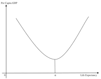
role for the transition from stagnation to growth” (page 103). For instance, this concept is seen graphically illustrated in Fig.1.

During infant stages of development, any improvements on the level of health lead to a fall in wealth because of the occurrence of the Malthusian population effect. The latter postulates an exponential expansion in population growth. Yet, this effect is only temporary as fertility is apt to drop. As further health improvements occur beyond the turning pointα, human capital accumulations and economic development are stimulated. This eventually causes population growth rate to fall (Hansen2012). Various studies have investigated the impact of life expectancy on economic growth. Acemoglu and Johnson (2007) find a negative but statistically insignificant impact whereas Zhang and Zhang (2005), Bloom et al. (2009), Turan (2009) and Aghion et al. (2010) uncover a significantly positive one. Hansen (2012) is among the first to provide evidence of a U-shaped relationship using a world panel of 119 countries throughout the period of 1940–1980. Yet, while the models used in literature rely heavily on cross-sectional studies which may not adequately capture the effects of health, some have employed panel data of little importance given to non-stationary series, which can lead to spurious inferences.

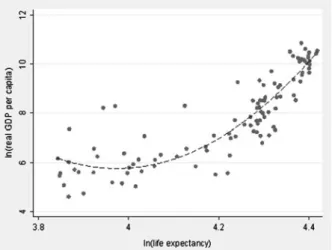
This paper revisits the implications of health on wealth by employing state-of-the-art panel data techniques. Using the 2011 World Development Indicators data from The World Bank Group, 107 countries for the 1970–2009 period are selected. Table1 shows the descriptive statistics for real gross domestic product (GDP) per capita (at constant 2000) and life expectancy at birth. Referring to Fig.2, the scatter plot for the year 2009 does reflect a slight U-shaped relationship between the two variables.

Results

To investigate whether a U-shaped relationship exists, the following quadratic re-gression is run:

LGDPit¼ b0þ b1LEXitþ b2LEXit2þ "it; ð1Þ

Per Capita GDP

0 Life Expectancy

where LGDPitdenotes the natural logarithm of real GDP per capita for country i and

year t and measures the level of wealth of in an economy. LEXitdenotes the natural

logarithm of life expectancy at birth for country i and year t. Also, it is used as a proxy for the general health conditions of a population (Acemoglu and Johnson2007).β1

andβ2estimate the impacts of life expectancy on real GDP per capita. If a U-shaped

relationship prevails between wealth and health levels, the expected outcomes will be β1<0 andβ2>0.β0is the constant term whileεitis the error term.

Prior to estimating the above equation, some preliminary tests are conducted. According to the Hausman’s (1978) specification test, the null hypothesis (H0) of

no systematic difference in coefficients between the fixed-effects (FE) and random-effects (RE) panel data models is rejected with the test statistics equal toχ2(2)= 245.68 [0.000]*. The FE panel data model best fits the data. The Greene (1993) groupwise heteroskedasticity test statistics are χ2(106) = 15955.74 [0.000]* and χ2

(106) = 15998.47 [0.000]* for the FE and RE panel data models respectively. Thus, the H0of homoskedasticity is rejected. Next, the Wooldridge (2002) no

first-order autocorrelation (AR(1)) test statistic is F(1,106)=289.25 [0.000]*. The H0is

rejected. The Pesaran (2004) test of H0no cross-sectional dependence (CSD) is equal

to 38.02 [0.000]* for the FE panel data model. The p-value is in square brackets. The presence of CSD is found. In addition to the FE and RE panel data models, the Prais and Winsten (1954) heteroskedastic panel corrected standard error model which can control for AR(1) specific to each panel is applied (StataCorp2007).

As exposed in Table4, the U-shaped hypothesis is supported. Since β1andβ2

are statistically significant at the 1 % level, a precise and meaningful value ofα can

Table 1 Descriptive statistics for the period 1970–2009

Data Mean Standard deviation Minimum Maximum

Real GDP per Capita ($) 6105.71 8738.81 57.78 56388.99

Life Expectancy (years) 63.68 11.46 26.82 82.93

Computed

be obtained from the models. For instance, a 99 % confidence interval for α is reported for the FE, RE, and PW panel data models. Allα’s are found to lie within this estimated interval. Their p-values are also computed to be 0.000, implying they are statistically significant from zero. Nevertheless, these three models are based on the stationarity assumption and ignore any non-stationary process of the series which can result in spurious inferences. Efficient models such as the fully modified ordinary least squares (FMOLS) model need be considered. Preliminary tests such as panel unit root and cointegration tests are accordingly required. When performing panel unit root tests, two distinct specifications are utilized. One test includes a constant term only while the other contains both a constant term and a time trend. Macroeconomic data tends to display a trend over time. It is more fitting to consider a regression with a constant and a trend at level form. Since first-differencing tends to extract any deterministic trends, inferences will be carried out by considering a constant term only.

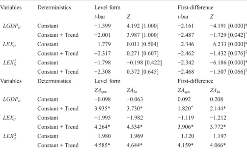
Pesaran (2007) recommends a test of the H0of a unit root which allows for the

presence of CSD patterns. To control for these patterns, the standard augmented Dickey-Fuller (ADF) regression models are augmented with the cross-sectional averages of the lagged levels and the first-differences of the individual series. The test is based on the cross-sectionally ADF (CADF) statistics. As revealed in Table2 (a), the results from the Pesaran test corroborate with the earlier tests. All variables are once more found to follow an I(1) process. Kwiatkowski et al. (1992) recommend a test of the H0of the stationarity hypothesis to complement the H0of a unit root. Such

joint testing is known as confirmatory analysis (Romero-Ávila2008). The test of the H0of stationarity as suggested by Hadri and Kurozumi (2012) is applied. This test

allows the Lagrange multiplier (LM) test to control for CSD. Although it is similar to the KPSS test, the regression is augmented by the cross-sectional average of the observations à la Pesaran (2007). As illustrated in Table2(b), both ZAspcand ZAlatest

statistics confirm an I(1) process for all three series.

Karlsson and Löthgren (2000) issue a caveat where the rejection of the panel unit root can be driven by a few stationary series and consequently the whole panel may erroneously be modelled as stationary. The Narayan and Popp (2010) time-series unit root tests1 of two breaks in the level and slope for LGDPit, LEXit and LEXit2 are

performed where 12, 17, and 13 countries are found to be I(0) respectively. Per se, the Pesaran (2007) test is redone by excluding those countries and no major difference to the results is found. The Westerlund (2007) cointegration tests are next performed. Ga and Gt test statistics test the H0of no co-integration for at least one of the

cross-sectional units. Pa and Pt test statistics use the pooled information over all of the cross-sectional units to test the H0of no co-integration for the whole panel. To control

for CSD, robust critical values are obtained through 5,000 bootstrap replications. As shown in Table3, H0is rejected when referring to the Gt and Pt test statistics. These

panel unit roots and cointegration tests form part of the second-generation tests as they can effectively control for CSD. The first-generation tests rely mainly on the assumption of cross-sectional independence.

1

The panel FMOLS estimates are presented in Table4. The latter can effectively deal with both serial correlation and heteroskedasticity of residuals while controlling for any potential endogeneity of regressors. For instance, while health improvements can be positively related to income, the reverse is also true. Higher incomes make healthy goods and services such as good nutritious diet, proper sanitation, high-tech Table 2 (a): Pesaran panel unit root test statistics (b): Hadri and Kurozumi panel unit root test statistics

Variables Deterministics Level form First-difference

t-bar Z t-bar Z LGDPit Constant −1.399 4.192 [1.000] −2.161 −4.191 [0.000]* Constant + Trend −2.001 3.987 [1.000] −2.487 −1.729 [0.042]+ LEXit Constant −1.779 0.011 [0.504] −2.346 −6.233 [0.000]* Constant + Trend −2.317 0.271 [0.607] −2.462 −1.432 [0.076]‡ LEX2 it Constant −1.798 −0.198 [0.422] −2.342 −6.186 [0.000]* Constant + Trend −2.308 0.372 [0.645] −2.468 −1.507 [0.066]‡

Variables Deterministics Level form First-difference

ZAspc ZAla ZAspc ZAla LGDPit Constant −0.098 −0.063 0.092 0.208 Constant + Trend 3.935* 3.730* 1.820+ _2.144* LEXit Constant −1.995 −1.982 −1.119 −1.212 Constant + Trend 4.264* 4.334* 3.906* 3.772* LEX2 it Constant −1.980 −1.969 −1.120 −1.197 Constant + Trend 4.585* 4.644* 4.159* 4.066*

Computed. Note: The Bartlett kernel which is equal to 4(T/100)2/9≈4 is used for the lag order. Critical

values for the t-bar statistics without and with trend at 1 %, 5 % and 10 % significance levels are−2.140,

−2.060 and −2.010; and −2.620, −2.540 and −2.500 respectively. The normalized Z test statistic is

compared to the 1 %, 5 % and 10 % significance levels with the one-sided critical values of−2.326,

−1.645 and −1.282 correspondingly. *,+

and ‡ denotes 1 %, 5 % and 10 % significance level

correspondingly. P-value is given in square brackets. The H0of stationarity is tested. The ZAspcand ZAla

test statistics are compared to the 1 %, 5 % and 10 % significance levels with the one-sided critical values of

2.326, 1.645 and 1.282 respectively. Following Kwiatkowski et al. (1992), the number of lags is set on the

order of T1/2≈7

Table 3 Westerlund panel cointegration test statistics

Statistics Without trend With trend

Value Z P-value Robust P-value Value Z P-value Robust P-value

Gt −2.737 −13.378 0.000* 0.000* −3.729 −14.769 0.000* 0.000*

Ga −4.076 3.306 1.000 0.037+ −4.489 12.901 1.000 1.000

Pt −16.084 −4.810 0.000* 0.000* −25.647 −2.199 0.014+ 0.027+

Pa −2.988 −1.033 0.151 0.001* −5.428 7.743 1.000 0.970

Computed. Note: All these statistics are distributed standard normally. Critical values of one-sided tests for

1 %, 5 % and 10 % significance levels are−2.326, −1.645 and −1.282 respectively. The lag and lead lengths

T able 4 Regressions Statistics F E R E P W F M OLS β0 1.19 72.9 8 0.71 74.33 − 6.13 63.5 7 –– (0.2 9)* (16.40) * (0.31) + (16.33) * (0.53)* (5.6 2)* –– β1 1.55 − 34.2 6 1.66 − 35.06 3.32 − 32.2 7 − 0.57 − 39.8 8 (0.0 7)* (8.09)* (0.07)* (8.05)* (0.13)* (2.8 0)* (− 1.41 ) ‡ (1.7 5)* β2 – 4.45 – 4.56 – 4.53 – 4.99 – (1.00)* – (0.99)* – (0.3 5)* – (0.2 2)* R 2 0.15 0.31 0.68 0.74 0.95 0.96 –– Greene ( 1993 ) 1433 3.29 * 5955 .74* 1432 1.66* 15998.47 * –– – – Pesaran ( 2004 ) 63.3 6* 38.0 2* 58.5 1* 31.928* –– – – Obse rvations 4280 4280 4280 4280 4280 4280 4280 4280 Countr ies 107 107 107 107 107 107 107 107 α – 46.9 1 – 46.53 – 35.1 5 – 54.3 8 C.I. – [40.09,5 3.73 ] – [39.89,5 3.18] – [31. 77,38.52 ] –– Comput ed. R 2 is the within-R 2 for FE and overall-R 2 for RE models. Standa rd errors are in par entheses. C.I. den otes a 9 9 % confide nce interval

medical care, etc., more accessible and generate greater longevity. Healthcare may potentially be considered as endogenous and this may produce biased estimates. Moreover, to control for CSD, common time dummies are included (Pedroni2001). A negative impact of health on wealth is first encountered. On the other hand, when considering the possibility of a non-linear relationship, wealth is found to be on a U-shaped path in the country level of health. Additionally, the panel FMOLS model reveals a turning point at around 54 years of life expectancy as compared to only 35 or 47 years as per the conventional models.

Conclusions

The paper investigates the relationship between wealth and health status using a world panel data for the period 1970–2009. A U-shaped relationship is uncovered. However, conventional estimators reveal a turning point of about 35 and 47 years, while a much greater value of 54 years is obtained when applying an efficient estimator such as the panel FMOLS. In sum, health effects on wealth are inclined to vary over different stages of economic development. Policymakers should therefore take for this non-monotonic relationship into account when designing healthcare schemes.

Appendix

List of countries: Algeria, Argentina, Australia, Austria, Bahamas, Bangladesh, Barbados, Belgium, Belize, Benin, Bolivia, Botswana, Brazil, Burkina Faso, Burundi, Cameroon, Canada, Central African Republic, Chad, Chile, China, Colombia, Congo DR., Congo Rep., Costa Rica, Cote d’Ivoire, Denmark, Dominican Rep., Ecuador, Egypt, Arab Rep., El Salvador, Fiji, Finland, France, Gabon, Gambia, Georgia, Germany, Ghana, Greece, Guatemala, Guinea-Bissau, Guyana, Honduras, Hong Kong, China, Hungary, Iceland, India, Indonesia, Iran Islamic Rep., Ireland, Israel, Italy, Jamaica, Japan, Kenya, Korea Rep., Latvia, Lesotho, Liberia, Luxembourg, Madagascar, Malawi, Malaysia, Mali, Malta, Mauritania, Mexico, Morocco, Nepal, Netherlands, Nicaragua, Niger, Nigeria, Norway, Oman, Pakistan, Panama, Papua New Guinea, Paraguay, Peru, Philippines, Portugal, Rwanda, Saudi Arabia, Senegal, Sierra Leone, Singapore, South Africa, Spain, Sri Lanka, St. Vincent and the Grenadines, Sudan, Swaziland, Sweden, Syrian Arab Rep., Thailand, Togo, Trinidad and Tobago, Tunisia, Turkey, United Kingdom, United States, Uruguay, Venezuela, Zambia, Zimbabwe.

References

Acemoglu, D., & Johnson, S. (2007). Disease and development: the effect of life expectancy on economic

growth. Journal of Political Economy, 115(6), 925–985.

Aghion, P., Howitt, P. & Murtin, F. (2010).“The relationship between health and growth: When Lucas

meets Nelson–Phelps,” NBER Working Paper 1581. Online at:http://www.ofce.sciences-po.fr/pdf/

dtravail/WP2009-28.pdf.

Bloom, D.E., Canning, D. & Fink G. (2009).“Disease and development revisited,” NBER Working Paper

Cervellati, M., & Sunde, U. (2011). Life expectancy and economic growth: the role of the demographic transition. Journal of Economic Growth, 16(2), 99–133.

Greene, W. H. (1993). Econometric analysis (2nd ed.). New York: Macmillan Publishing Company. Hadri, K., & Kurozumi, E. (2012). A simple panel stationarity tests in the presence of cross-sectional

dependence. Economics Letters, 115(1), 31–34.

Hansen, C. W. (2012). The relation between wealth and health: evidence from a world panel of countries.

Economics Letters, 115(2), 175–176.

Hausman, J. A. (1978). Specification tests in econometrics. Econometrica, 46(6), 1251–1272.

Karlsson, S., & Löthgren, M. (2000). On the power and interpretation of panel unit root tests. Economics

Letters, 66(3), 249–255.

Kwiatkowski, D., Phillips, P., Schmidt, P., & Shin, Y. (1992). Testing the null hypothesis of stationarity

against the alternative of unit root. Journal of Econometrics, 54(1–3), 159–178.

Narayan, P. K., & Popp, S. (2010). A new unit root test with two structural breaks in level and slope at

unknown time. Journal of Applied Statistics, 37(9), 1425–1438.

Pedroni, P. (2001). Purchasing power parity tests in cointegrated panels. The Review of Economics and

Statistics, 83(4), 727–731.

Pesaran, M.H. (2004).“General diagnostic tests for cross section dependence in panels.” Cambridge

Working Papers in Economics, 0435, Online at: http://www.econ.cam.ac.uk/faculty/pesaran/

CDtestPesaranJune04.pdf.

Pesaran, M. H. (2007). A simple panel unit root test in the presence of cross-section dependence. Journal of

Applied Econometrics, 22(2), 265–312.

Prais, S.J. & Winsten C.B. (1954).“Trend Estimation and Serial Correlation.” Cowles Commission

Discussion Paper No. 383, Chicago.

Romero-Ávila, D. (2008). A confirmatory analysis of the unit root hypothesis for OECD consumption

income ratios. Applied Economics, 40(17), 2271–2278.

StataCorp. (2007). Stata Statistical Software: Release 10. College Station: StataCorp LP.

Turan, B. (2009).“Life Expectancy and economic development: Evidence from micro data.” Working

Paper. Online at:http://www.uh.edu/~bkturan/lifeexpec.pdf.

Westerlund, J. (2007). Testing for error correction in panel data. Oxford Bulletin of Economics and

Statistics, 69(6), 709–748.

Wooldridge, J. M. (2002). Econometric analysis of cross section and panel data. Cambridge: MIT Press. Zhang, J., & Zhang, J. (2005). The effect of life expectancy on fertility, saving, schooling and economic