A laboratory study of tracer tomography
R. Brauchler&G. Böhm&C. Leven&P. Dietrich&M. Sauter
Abstract A tracer tomographic laboratory study was performed with consolidated fractured rock in three-dimensional space. The investigated fractured sandstone sample was characterized by significant matrix permeabil-ity. The laboratory transport experiments were conducted using gas-flow and gas-tracer transport techniques that enable the generation of various flow-field patterns via adjustable boundary conditions within a short experimen-tal time period. In toexperimen-tal, 72 gas-tracer (helium) tests were performed by systematically changing the injection and monitoring configuration after each test. For the inversion of the tracer breakthrough curves an inversion scheme was applied, based on the transformation of the governing transport equation into a form of the eikonal equation. The reliability of the inversion results was assessed with singular value decomposition of the trajectory density matrix. The applied inversion technique allowed for the three-dimensional reconstruction of the interstitial velocity with a high resolution. The three-dimensional interstitial velocity distribution shows clearly that the transport is dominated by the matrix while the fractures show no apparent influence on the transport responses.
Keywords Tracer tests . Hydraulic tomography . Inverse modeling . Fractured rocks . Laboratory experiments/ measurements
Introduction
Investigation methods that allow for the characterization of hydraulic subsurface properties, for example, the continuity of preferential flow paths or the presence of hydraulic barriers, are of great interest for the prediction of solute transport in the subsurface (Butler 2005). The concept of hydraulic tomography has been introduced by several working groups over the last two decades (e.g. Tosaka et al. 1993; Gottlieb and Dietrich 1995; Yeh and Liu 2000). Hydraulic tomography can be described by a series of short-term hydraulictests, whereby the location of the source stress (pumping or slug interval) and the receivers (pressure transducers) are varied between the tests. The set-up was based on the concept of medical and geophysical tomography and facilitates a high-resolution characterization of hydraulic subsurface parameters, hy-draulic conductivity (K) and storage (S) in two and three dimensions. In the lastfive years, the developed inversion schemes have been increasingly applied to field data recorded for unconsolidated sediments. Depth integrated reconstructions of K- and S-fields, based on the inversion of pumping tests data, are shown by Straface et al. (2007); Cardiff et al. (2009), and Huang et al. (2011). Brauchler et al. (2010) reconstructed a two-dimensional (2D) vertical diffusivity profile utilizing data from cross-well interfer-ence slug tests. Reconstructions of three-dimensional (3D) K- and S-fields were reported by Li et al. (2008); Brauchler et al. (2011); Berg and Illman (2011) and Cardiff et al. (2012). The only large-scalefield assessment was performed by Illman et al. (2009). They inverted two large-scale pumping tests in a granite aquifer and computed the K- and S-parameter field in three-dimen-sions. Brauchler et al. (2012) exploited the high spatial resolution of the hydraulic and geophysical tomographic images to define site-specific relationships between hy-draulic and geophysical parameters.
The afore-mentioned field studies demonstrated that hydraulic tomography is a suitable method to provide high-resolution images about the subsurface heterogeneity
Received: 18 October 2012 / Accepted: 24 May 2013 Published online: 9 June 2013
* Springer-Verlag Berlin Heidelberg 2013 R. Brauchler ())
ETH Zurich, Department of Earth Sciences, Sonneggstrasse 5, 8092 Zurich, Switzerland
e-mail: [email protected] Tel.: +41-44-6332147
Fax: +41-44-6331108 G. Böhm
OGS– Istituto Nazionale di Oceanografia e di Geofisica Sperimentale, Borgo Grotta Gigante 42/c,
34010 Sgonico, Trieste, Italy C. Leven
:
P. DietrichUniversity of Tübingen, Center of Applied Geoscience, Sigwartstraße 10, 72076 Tübingen, Germany
P. Dietrich
UFZ, Helmholtz Centre for Environmental Research, Department Monitoring and Exploration Technologies, Permoserstrasse 15, 04318 Leipzig, Germany
M. Sauter
Geoscientific Centre, University of Göttingen, Goldschmidtstraße 3, 37077 Göttingen, Germany
of K and S and that the method is beginning to develop into a robust field method. Besides the necessity for the information on the hydraulic parameters, the knowledge about transport parameters (porosity, transport velocity, dispersivity) is also essential for the prediction of solute transport.
The conventional way to determine transport parame-ters is to conduct tracer experiments (e.g. Ptak et al.2004). Similar to the concept of hydraulic tomography the significance of tracer test results could be greatly increased with respect to spatial resolution of the estimated transport parameters by injecting and monitor-ing the tracer at different locations to produce a pattern of crossing transport paths. There are only a few studies, to the authors’ knowledge, about tracer tomography. Yeh and Zhu (2007) developed a hydraulic/partitioning tracer tomographic inversion approach to characterize dense non-aqueous phase liquid (DNAPL) source zones. The inversion algorithm adopted a stochastic information fusion concept (Yeh and Simunek 2002) in a way that the information content of hydraulic tomography, as well as tracer tomography, is exploited in a single inversion. Zhu et al. (2009) further developed the inversion algorithm in order to reduce the computational effort by fitting temporal moments of the tracer breakthrough curves instead of discrete concentration data. Illman et al. (2010) applied the inversion technique to a small-scale sandbox experiment and could show the importance of the knowledge of the hydraulic conductivity field for the location of the DNAPL source zone. Vasco and Datta-Gupta (1999) proposed an asymptotic approach based on the transformation of the governing transport equation into a form of the eikonal equation, describing the propagation of a solute tracer concentration in space and time. The application to a conservative tracer test indicated the potential of the approach, especially when matching tracer arrival times, for characterizing variations in permeability and porosity. Datta-Gupta et al. (2002) further developed this approach and applied it to partitioning inter-well tracer tests to identify the location and distribution of non-aqueous phase liquids.
In this study, a tomographic laboratory study was performed on a cubic sandstone block of 60 × 60 × 60 cm3 in size. Such laboratory experiments are an efficient way to develop, test and validate new investigation technologies. Particularly, the possibility to validate the reconstructed parameter fields is a big advantage over in situ testing (Illman et al. 2010). The investigated cubic sandstone block is known to have a significant matrix permeability in the order of 10−12–10−15m2(e.g. Hornung and Aigner 2002). The transport experiments were conducted using a gas flow and gas tracer experimental technique that enables the generation of a multitude of flow field patterns by changing the boundary conditions. A similar experimental set-up was utilized by McDermott et al. (2003), Brauchler et al. (2003) and Leven et al. (2004) for the tomographic investigation of lab-scale fractured sandstone blocks with the aim to reconstruct flow parameters with a high spatial resolution. In this
study, 72 gas tracer tests were performed by changing the injection and monitoring position after each test. The performed inversion of the tracer breakthrough curves is based on the transformation of the governing transport equation into a form of the eikonal equation developed by Vasco and Datta-Gupta (1999). The inversion technique allowed for the 3D reconstruction of the interstitial velocity of the sandstone block with a high resolution.
The structure of this paper is as follows: the method-ology on which the applied tomographic inversion technique is based is introduced first. The experimental set-up and the statistical description of the recorded breakthrough curves are given, after which the inversion parameters and the reconstructed tracer velocity tomo-grams are presented. Finally, thefindings are summarized and there is a discussion of the potential and limitations of the method.
Methodology
Vasco and Datta-Gupta (1999) showed that the transport equation can be transformed into a form of the eikonal equation using an asymptotic extension to the governing transport equation. Hence, the spreading of a tracer pulse can be treated as a front of concentration, which can be described by trajectories arranged perpendicular to the concentration front. The introduction of a curvilinear coordinate system aligned along the trajectories reduces the 3D to a one-dimensional (1D) inverse problem. For the definition of the trajectory, constraints are given by the test set-up. The trajectory starts at the injection point x1 and ends at another specified observation point x2. Based on this, Vasco and Datta-Gupta (1999) defined a line integral, which relates the tracer arrival time tt to the
slowness (i.e. the inverse of the velocity v) of the tracer along the trajectory s.
ttð Þ ¼ ∫x2 x2
x1 ds
v sð Þ: ð1Þ
By utilizing the peak arrival time of a conservative tracer, assuming a Dirac pulse injection, the slowness is identical to the interstitial/mean velocity vm and can be
expressed as follows by:
ttð Þ ¼ ∫x2 x2 x1 ds vmð Þs ¼ ∫ x2 x1 n sð Þ K sð Þϕ sð Þds; ð2Þ
where n is the porosity, K hydraulic conductivity and Φ the potential head. Equation2relates the peak arrival time of a conservative tracer to the interstitial velocity. In this manner, the interstitial velocity is assumed locally as homogeneous and thus the whole trajectory is a sum of a defined number of homogeneous sections.
Experimental set-up and database
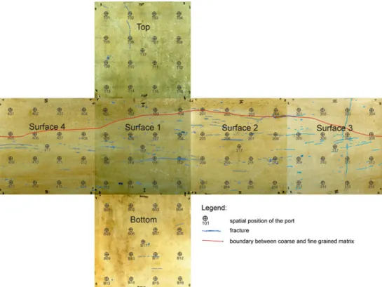
A sandstone block of 60 × 60 × 60 cm3 in size was recovered from the upper part of the Triassic Stubensandstein Formation, which is quarried in southern Germany. This formation displays a continental alluvial depositional system (Hornung and Aigner 1999) and is characterized by high matrix porosity and a dense regularly spaced fracture network. The sample itself reflects a bed load channel-dominated facies. After the recovery, the block was cut to a cubic shape, which enables the definition of geometrical boundaries. The sandstone block was dried for several weeks in a heated room. For later interpretation and validation purposes, the petrofabrics and fracture network of the block surfaces was mapped in detail using a polyethylene foil. Figure 1 displays photographs of the six cube faces and the identified petrofabric and fracture network.
To access the block forflow and transport experiments, 17 ports with three centimeters in diameter were attached in a regular grid on each side of the block. The ports consist of circular metal fittings and valves that allow for access to a controlled area of the block. Finally, the block was sealed with six different coats of epoxy resin, that could stand pressures of up to three bar. A detailed description of the preparation procedure can be found in Leven et al. (2004,2005).
In order to characterize thefissured sandstone block in terms of heterogeneity and anisotropy, flow and transport experiments were conducted using a gas flow and gas transport technique developed by McDermott (1999) and McDermott et al. (2003). The main reason for utilizing the gas flow/tracer technique was that flow and transport experiments can be performed much faster in comparison to hydraulic testing and solute transport experiments. In order to guarantee the transformation to water saturated systems, the experiments were designed in a way that gas compressibility can be neglected.
The experimental set-up for tracer testing is displayed in Fig. 2. First, compressed air is injected into the sandstone block through one port and theflow rate is measured at the port at the opposite block face using a mass-flow meter. Second, a gas tracer (helium) is injected via a bypass loop after a stationaryflow field was established. The concentra-tion at the observaconcentra-tion port was detected using a mass spectrometer. During the individual experiments, a pressure difference between injection and observation port of 0.5 bar was applied and 1.05×10⁻⁴ m3 helium was injected. As shown by Brauchler et al. (2003) the effects of compress-ibility can be neglected for a pressure difference of 0.5 bar over a distance of 0.6 m.
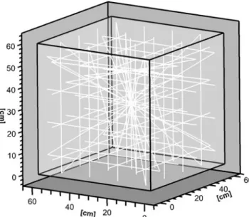
In total, 72 tracer breakthrough curves were recorded using the experimental set-up described in the preceding. Figure 3 presents the measured configurations, whereby the injection and observation port are connected by a line. The measurement density was increased in the upper part of the block in order to receive more information about the spatial position of the boundary between the coarse-grained matrix characterizing the upper part and the finer
grained matrix characterizing the lower part of the sandstone block (Fig. 1). The recorded breakthrough curves are very diverse although the transport distance (assuming a straight line between injection and observa-tion port) only varies between 0.6 m and 0.87 m. Moreover, the high variability in the shape of the breakthrough curves (Fig. 4) are reflected in the great variety of the peak arrival time (time of maximum concentration) ranging from 335 to 12,361 s.
For the parameters mean tracer velocity andflow rate, a histogram and a boxplot is shown in Fig. 5. Both histograms (Fig. 5a,b) show a similar distribution and the mode of both parameters is around 10−4 m/s and 100 ml/min. These values are associated with experiments, where either the injection or the extraction port is located in the fine-grained matrix, i.e. in the lower part of the block. Values which are strongly higher are indicated as outliers in the boxplots (Fig.5c, d). Note the outliers are defined as a point that falls below QL-1.5×IQR or above QL-1.5×IQR, whereby IRQ is the difference between the quartiles, QL is the value of the lower quartile and QU is the value of the upper quartile. These values that are marked as outliers are associated with experiments, where both the injection and the extraction port are located in the coarse-grained matrix, i.e. in the upper part of the block.
Inversion
The propagation of a seismic signal can be described similarly to that of Eq. 2, by a line integral relating the travel time ts, recorded between a source and a receiver,
with the spatial seismic velocity distribution vs of an
investigated area: tsð Þ ¼ ∫x2 x2 x1 ds vsð Þs ; ð3Þ
where x1and x2denote the positions of the source and the
receiver, respectively. The line integral is solved using well-established eikonal solvers such as LSQR (Paige and Saunders1982), ART (Gordon1979) or SIRT algorithms (Gilbert1972).
For the inversion of the tracer breakthrough curves the similarity between Eqs.2and3was exploited and an eikonal solver based on the SIRT algorithm was used. InAppendix 1, a summary of the SIRT algorithm with regard to the inversion of tracer breakthrough curves is given. In geophysical ray tomography, the velocity contrasts do not exceed 20 to 30%. However, in tracer tomography, velocity contrasts of several orders of magnitude are observed. Hence, ray tracing techniques that have been proven to improve the reliability of the inversion characterized by high velocity contrasts (e.g. Dines and Lytle1979; Peterson et al. 1985) were applied. The applied ray tracing technology is based on the minimum-time principle. The starting point is a straight trajectory connecting source and receiver. At each
cell boundary the trajectory is divided by inserting a point, which can be moved along the boundary between two adjacent cells. The optimization, based on Snell’s law, starts at the point closest to the source and is applied then, step by step, to all other points defining the trajectory. The goal of the optimization is to minimize the travel time of the induced signal. After the correction for all points of a trajectory, the optimization will be repeated starting from the point closest to the receiver. The procedure is applied until the difference between the trajectory of the previous iteration and the last
calculated one is lower than a chosen threshold. In Appendix 2, the applied minimum-time algorithm is explained in detail.
To assess the reliability of the tomographic model, the null-space energy map of the area of the model domain was computed. The null-space energy map represents a measure of the reliability of a tomographic system, because it relates the trajectory distribution to the mesh used for the discretization of the investigated area. In the following, a short description of the calculation of the
Fig. 1 Photographs of the six faces of a 0.60×0.60×0.60 m3cubic sandstone block and overlain maps of the petrofabric and fracture
network
null-space energy map is given, which is based on the work of Böhm and Vesnaver (1996). The null-space energy map comprises a singular value decomposition of the tomographic matrix A, where Aij of the matrix A are
the lengths of the ith trajectory path in the jth voxel (compare Appendix 1). This matrix can be factorized into three components:
A¼ UWVT ð4Þ
The squared matrices U and V are orthonormal:
U UT¼ I; V VT¼ I ð5Þ
The elements wiiof the diagonal matrix W are the singular
values corresponding to the square of the eigenvalues. The
stability of the tomographic inversion is defined by the elements wii. Small singular values indicate instabilities. The
singular values according to their numerical value were recognized. Taking into account that the columns of the matrix Vof the decomposition (Eq.4) display an orthonormal basis of the model domain, the local reliability, R, of each voxel can be defined as the summation of the squared elements viof the matrix V:
R ¼ Σiv2i ð6Þ
The summation of the elements is equal to one if the index i covers the whole model domain and each voxel is associated with a value ranging from 0 to 1. Voxels associated with high values of null space energy reflect high uncertainty and vice versa. For further details on the significance and derivation of the null-space energy map, please see Böhm and Vesnaver (1996).
For the tracer tomographic inversion, a homogeneous starting model was employed. The starting values for the interstitial velocityfield are derived from the mean values of the measured source-receiver-combinations. For the inversion of the travel time signals derived from the tracer breakthrough curves, the SIRT algorithm (Appendix 1) and the ray-bending algorithm based on the minimum time principle (Appendix 2) were used. For the initial model domain, a relatively coarse grid of 4×4×6 voxels is chosen, because the applied inversion scheme includes no regularization terms. The adaptation of the number of measurements (breakthrough curves) to the number of unknowns (voxels) allows for the formulation of an even-determined inverse problem.
In order to increase the nominal resolution of the coarse grid, the staggered grid method developed by Vesnaver and Böhm (2000) was utilized. The method combines the advantages of low-resolution grids (stable inversion) with the need of high-resolution information. The method is based on the displacement of the initial grid in all directions. The displacement rates Δx, Δy, Δz are one third of the voxel length in the x-, y- and z-directions, respectively. For each grid position, a slightly different image was obtained, because inside each voxel the interstitial velocity over a different volume was averaged. In all, 64 inversions were performed and the arithmetic mean of all grids was determined by staggering them. As a result, the final grid is composed of 16 voxels in the x-and y-directions x-and 24 voxels in the z-direction.
Results
Slices of the interstitial tomogram of the cubic sandstone block are displayed in Fig. 6. For a good comparison between the detailed mapping of the petrofabric and fracture network of the surfaces and the reconstructed interstitial velocity four slices in the x-direction (Fig.6a–f) and four slices in the y-direction were visualized (Fig.6k–p), as well
Fig. 3 Tomographic measurement overview. The respective injection and observation ports are connected by a white line
as the respective photographs of the block surfaces. For the interpretation, the respective null space energy distribution is displayed below each reconstructed interstitial velocity slice (Fig.6g–j, q–t). Note the null-space energy map represents a measure of the reliability of a tomographic system because it relates the trajectory distribution to the mesh used for the discretization of the investigated area. This allows for the evaluation of the reliability of the reconstructed features in the reconstructed interstitial velocity distributions. All slices have in common that the highest interstitial velocity are reconstructed in the upper part between levels z=45 and z= 55 cm. This agrees with the spatial position of the coarser grained matrix, which can be assumed to be more permeable. However, the area between levels z=55 cm and z=60 cm is characterized again by slightly lower values, which are not in accordance with the surface mapping. The decrease can be explained with poor trajectory coverage close to the surfaces of the block (Fig.3). The poor coverage is also reflected by the null space energy maps showing the lower values in this part in contrast to the area between levels z=45 and z=55 cm. Hence, the area between levels z=55 cm and z=60 cm should be not over- interpreted and additional information in this part is required to perform afinal evaluation if the zone characterized with the highest interstitial velocity values stretches out to the upper border of the block. However, the area between levels z=45 and z=55 cm is in agreement with
the lowest null space energy values, which indicates the high reliability of the existence of this zone.
The lowest values are reconstructed mainly between levels z=20 and z=40 cm, which agrees partly with the area of highest fracture density. Although there is no clear relationship between the individually mapped fractures and lower interstitial velocity values, it can be concluded that fractures are not acting as preferentialflow paths. Hence, the fractures are either not interconnected or arefilled with low permeability material (fault gouge), which was however not always obvious during the surface mapping.
Conclusion
In this study, a travel-time-based tomographic inverse scheme to tracer breakthrough curves recorded at a cubic sandstone block with an edge length of 0.6 m was applied. In total, 72 forced gradient gas tracer experiments were performed. Thereby, compressed air was utilized to establish a steady-stateflow field and helium was injected by a Dirac pulse via a bypass loop.
The inversion scheme is based on the transformation of the general form of the governing transport equation into a form of the eikonal equation as introduced by Vasco and Datta-Gupta (1999). The similarity between geophysical
ray tomography and the tracer tomographic approach was exploited and an eikonal solver (SIRT algorithm) and a ray bending algorithm based on the minimum-time principle for the inversion was utilized. Both techniques are well established in geophysical ray tomography and have a high computationally efficiency. For the assessment of the reliability of the reconstructed image of the interstitial velocity distribution, the null space energy map was calculated. The null space energy map is based on singular value decomposition and allows for an evaluation of the reconstructed tomogram by quantifying the relationship between trajectory distribution and the mesh used for discretization. Although the transformation of the governing transport equation into a form of the eikonal equation is an approximation, it could be shown that the applied inversion scheme allows for the 3D reconstruction of the interstitial velocity distribution. Particularly, the spatial agreement of the upper part of the sandstone block, characterized by a coarser-grained matrix, with the highest values of the interstitial velocity tomogram demonstrates
the high potential of the inversion scheme and interpreta-tion strategy. Furthermore, the lowest null space energy values were calculated in the upper part of the sandstone, which indicates the high reliability of the existence of this zone characterized by high interstitial velocity values. However, the potential of the method to detect more disseminatedflow-connectivity pathways, such as fracture networks, has to be further investigated.
The combination of hydraulic tomography and tracer tomography is a worthwhile topic for future research. Several researchers showed that hydraulic tomography is a characterization method that enables the reconstruction of the hydraulic properties diffusivity, hydraulic conductivity and storage with a high spatial resolution in thefield (Li et al. 2008, Brauchler et al.2011;2013; Berg and Illman 2011; and Cardiff et al. 2012). If the hydraulic conductivity and interstitial velocity distribution can be reconstructed with a high spatial resolution then it is possible to derive the porosity distribution using Eq. (2). Hence, a further important parameter next to hydraulic conductivity and
Fig. 6 Comparison of the surface mapping (a, f, k, p) with the reconstructed interstitial velocity distribution: b–e display slices of the reconstructed 3D interstitial velocity distribution in the x-direction and l–o in the y-direction; g–j show the associated null space energy maps in the x-direction and q–t show these in the y-direction
storage could be determined, which would be a further step of improvement in terms of solute transport prediction in the subsurface. Similar to the work in hydraulic tomography that was started one decade ago with laboratory experiments (Brauchler et al. 2003), the intension is to transfer the presented approach to thefield. Note, the tracer tomographic inversion approach can be applied without any restrictions to real aquifers, keeping in mind that pneumatically and hydraulically initiated tracer tests are based on the same flow equations if compressibility can be neglected. For the field implementation, it is intended to utilize the continuous multi-channel tubing (CMT) system (Einarson and Cherry 2002). This system was originally developed for multi-level sampling and consists of a pipe with seven continuous separate channels or chambers (ID=0.014 m), which are arranged in a honeycomb shape. In each individual chamber an opening, covered with a sandfilter, is cut. Such a system is perfectly suited for the performance of a tracer tomo-graphic experiment because no packer system has to be moved and cross-contamination effects can be excluded.
Tracer tomography could become a valuable tool for investigation of the excavation damage zone of under-ground constructions, monitoring of clogging processes during artificial recharge, or observing the change of hydraulic properties of permeable reactive barriers, which may occur due to chemical processes. A small investiga-tion scale is also sufficient for cases where a dense well network is available, e.g. at control planes used for contaminant site characterizations.
Acknowledgements The investigations were conducted with the financial support of the Swiss National Science Foundation to the project“A field assessment of high-resolution aquifer characteriza-tion: an integrated approach combining hydraulic tomography and tracer tomography” under grant number 200021_140450 / 1 and the financial support of the German Research Foundation to the project “Hard Rock Aquifer Analogue: Experiments and Modeling” project under grant DI833/1-4.
Appendix 1: SIRT algorithm
The description of the SIRT algorithm with regard to the inversion of tracer breakthrough curves, given in the following, is partly based on the work proposed by Dines and Lytle (1979) and by Hu et al. (2011) in context of the inversion of seismic signals and hydraulic transient pressure signals, respectively.
The interstitial or mean velocity vm of a conservative
tracer can be expressed by the following line integral, which relates the peak arrival time of a conservative tracer, assuming a pulse injection, to the ratio between porosity and hydraulic conductivity K multiplied by the potential headΦ (Vasco and Datta-Gupta, 1999):
ttð Þ ¼ ∫x2 x2 x1 n sð Þ K sð Þϕ sð Þds ¼ ∫ x2 x1 ds vmð Þs ; ð7Þ
where tt is the travel time of the peak of a tracer signal
between point x1 (source) and the observation point x2 (receiver) along the propagation path (s).
The integral (Eq.7) can be transformed into a discrete inverse problem by approximating the integral with a summation tt;i¼ ∑ n j¼1 1 vm;jdij ð8Þ
where dijis the distance along trajectory i in cell j and vm,j
is the average interstitial velocity within cell j. The applied SIRT algorithm for solving Eq.(8) is based on an iterative technique, where one equation (one trajectory) is analysed at a time. The algorithm requires an initial estimate of the average interstitial velocity. The interstitial velocity is calculated along each trajectory as follows:
tt;i¼ ∑ n j¼1
1
vqm;jdij; ð9Þ
where vm,jq indicates the estimated interstitial velocity
after the qth iteration. The applied SIRT algorithm minimizes for each source-receiver configuration the least squares residual between the predicted and the measured peak tracer arrival time,
Δtt;i¼ tmt;i−tet;i
h i ¼ ∑n j¼1 Δ 1 vqm;j dij ! ð10Þ with tt,imthe measured travel time, tt,iethe estimated travel
time,Δtt,ithe difference of the ith measured and estimated
peak tracer arrival time and tm
t;i describes the applied
changes to cell j of the qth iteration. Following Dines and Lytle (1979) an additional minimum criterion can be defined for the determination of the distribution ofv1q
m;j: f Δ 1 vqm;j ! ¼ ∑n j¼1 Δ 1 vqm;j !2 →min: ð11Þ
Minimizing the function f subject to Eq. (10) yields an update of the interstitial velocity for each cell sampled by trajectory i. For the minimization the Lagrange multipliers method can be utilized. Thereby the new function K is minimized: K ¼ ∑n j¼1 Δ 1 vqm;j !2 −lΔ 1 vqm;j di;j 2 4 3 5 þ lΔtt;i ð12Þ
Thefirst derivative becomes zero if:
Δ 1
vqm;j¼ ldi;j
Substituting Eq.(13) into Eq.(10) 1 can be expressed as follows: l ¼ X2nΔtt;i j¼1 d2i;j ð14Þ
The final solution is achived by substituting Eq. (14) into Eq.(13). The Lagrange multipliers method leads for a particular trajectory i, in the qth iteration to the incremen-tal correction: Δ 1 vqm;j ¼ Δtt;idij Xn j¼1 d2ij ð15Þ
The corrections are applied by averaging the incremental corrections of each single cell after all N trajectories have been analysed: Δ 1 vqm;j ¼ 1 Mj ∑ N i¼1Δ 1 vqm;j ð16Þ
where Mjis the number of trajectories passing through cell j.
Appendix 2: minimum time principle
Figure 7 displays two points A and B that are located in two half-spaces. The two half-spaces are characterized by their velocities v1and v2. In order to minimize the travel
time of an induced signal traveling between point A and B, a third point P located on the interface between the two half-spaces is introduced. The travel time between A and B can be expressed as follows:
f xð Þ ¼ ffiffiffiffiffiffiffiffiffiffiffiffiffiffiffi a2þ x2 p v1 þ ffiffiffiffiffiffiffiffiffiffiffiffiffiffiffiffiffiffiffiffiffiffiffiffiffiffi ab2þ c−xð Þ2 q v2 ð17Þ The minimum travel time can be found by setting thefirst derivative to zero: f0ð Þ ¼ bx 2þ c−xð Þ2 h i x2− v 2 1ðc−xÞ 2 a2þ x2 ð Þ h i v22 ¼ 0 ð18Þ The value x can be determined with the bisection method.
References
Berg SJ, Illman WA (2011) Three-dimensional transient hydraulic tomography in a highly heterogeneous glaciofluvial aquifer-aquitard system. Water Resour Res 47:W10507. doi:10.1029/ 2011WR010616
Böhm G, Vesnaver A (1996) Relying on a grid. J Seism Explor 5:169–184
Brauchler R, Liedl R, Dietrich P (2003) A travel time based hydraulic tomographic approach. Water Resour Res 39(12):1370
Brauchler R, Hu R, Vogt T, Al-Halbouni D, Heinrichs T, Ptak T, Sauter M (2010) Cross-well slug interference tests: an effective characterization method for resolving aquifer heterogeneity. J Hydrol 384(1–2):33–45
Brauchler R, Hu R, Dietrich P, Sauter M (2011) Afield assessment of high resolution aquifer characterization based on hydraulic travel time and hydraulic attenuation tomography. Water Resour Res 47:W03503
Brauchler R, Doetsch J, Dietrich P, Sauter M (2012) Derivation of site-specific relationships between hydraulic parameters and p-wave velocities based on hydraulic and seismic tomography. Water Resour Res 48:W03531. doi:10.1029/ 2011WR010868
Brauchler R, Hu R, Hu L, Jimenez S, Bayer P, Ptak T (2013) Rapid field application of hydraulic tomography for resolving aquifer heterogeneity in unconsolidated sediments. Water Resour Res. doi:10.1002/wrcr.20181
Butler JJ Jr (2005) Hydrogeological methods for estimation of hydraulic conductivity. In: Rubin Y, Hubbard S (eds) Hydrogeophysics. Dordrecht, Springer
Cardiff M, Barrash W, Kitanidis PK, Malama B, Revil A, Straface S, Rizzo E (2009) A potential-based inversion of unconfined steady-state hydraulic tomography. Ground Water 47(2):259– 270. doi:10.1111/j.1745-6584.2008.00541.x
Cardiff M, Barrash W, Kitanidis PK (2012) Afield proof-of-concept of aquifer imaging using 3D transient hydraulic tomography with modular, temporarily-emplaced equipment. Water Resour Res 48:W05531. doi:10.1029/2011WR011704
Datta-Gupta A, Yoon S, Vasco DW, Pope GA (2002) Inverse modeling of partitioning interwell tracer tests: a streamline approach. Water Resour Res 38(6):1079
Dines KA, Lytle RJ (1979) Computerized geophysical tomography. Proc IEEE 67(7):1065–1073
Einarson MD, Cherry JA (2002) A new multilevel ground water monitoring system using multichannel tubing. Ground Water Monit Rem 22(4):52–65
Gilbert P (1972) Iterative methods for three-dimensional reconstruction of an object from projections. J Theor Biol 36:105–117
Gordon R (1979) A tutorial on ART (algebraic reconstruction techniques). IEEE Trans Nucl Sci NS-21(17):78–93
Gottlieb J, Dietrich P (1995) Identification of the permeability distribution in soil by hydraulic tomography. Inverse Problems 11:353–360
Hornung J, Aigner T (1999) Reservoir and aquifer characterization of fluvial architectural elements: Stubensandstein, Upper Triassic, southwest Germany. Sediment Geol 129:215–280 Hornung J, Aigner T (2002) Reservoir architecture in a terminal
alluvial plain: an outcrop analogue study (Upper Triassic, Southern Germany), part 1: sedimentology and petrophysics. J Pet Geol 25(1):3–29
Hu R, Brauchler R, Herold M, Bayer P (2011) Hydraulic tomography analog outcrop study: combining travel time and steady shape inversion. J Hydrol 409(1–2):350–362. doi:10.1016/j.jhydrol.2011.08.031
Huang S-Y, Wen C, Yeh T-CJ LW, Juan H-L, Tseng C-M, Lee J-H, Chang K-C (2011) Robustness of joint interpretation of sequential pumping tests: numerical and field experiments. Water Resour Res 47:W10530. doi:10.1029/2011WR010698
Illman WA, Liu X, Takeuchi S, Yeh TJ, Ando K, Saegusa H (2009) Hydraulic tomography in fractured granite: Mizunami Underground Research site. Japan Water Resour Res 45:W01406
Illman WA, Berg SJ, Liu X, Massi A (2010) Hydraulic/partitioning tracer tomography for DNAPL source zone characterization: small-scale sandbox experiments. Environ Sci Technol 44:8609–8614
Leven C, Sauter M, Teutsch G, Dietrich P (2004) Investigation of the effects of fractured porous media on hydraulic tests: an experimental study at laboratory scale using single well methods. J Hydrol 297:95–108
Leven C, Brauchler R, Dietrich P (2005) Experiments: laboratory block. In: Dietrich P, Helmig R, Sauter M, Hötzl H, Köngeter J, Teutsch G (eds) Flow and transport in porous fractured media. Springer, Berlin, 25 pp
Li W, Englert A, Cirpka OA, Vereecken H (2008) Three-dimensional geostatistical inversion offlowmeter and pumping test data. Ground Water 46(2):193–201
McDermott CI (1999) New experimental and modelling techniques to investigate the fractured porous system, Tübinger Geowiss. Arb., Reihe C, 52, Cent. for Appl. Geosci., Tübingen, Germany, 166 pp
McDermott C, Sauter M, Liedl R (2003) New experimental techniques for pneumatic tomographical determination of the flow and transport parameters of highly fractured porous rock samples. J Hydrol 278:51–63
Paige CC, Saunders MA (1982) LSQR: an algorithm for sparse linear equations and sparse least squares. TOMS 8(1):43–71 Peterson JE, Paulsson BNP, McEvilly TV (1985) Application of
algebraic reconstruction techniques to crosshole seismic data. Geophysics 50:1566–1580
Ptak T, Piepenbrink M, Martac E (2004) Tracer tests for the investigation of heterogeneous porous media and stochastic modelling of flow and transport: a review of some recent developments. J Hydrol 29:122–163
Straface S, Yeh T-CJ, Zhu J, Troisi S, Lee CH (2007) Sequential aquifer tests at a wellfield, Montalto Uffugo Scalo, Italy. Water Resour Res 43:W07432
Tosaka H, Masumoto K, Kojima K (1993) Hydropulse tomography for identifying 3-D permeability distribution. High Level Radioactive Waste Management Proceedings of the Fourth Annual International Conference, Las Vegas, NV, April 1993, ASCE, Reston, VA
Vasco DW, Datta-Gupta A (1999) Asymptotic solutions for solute transport: a formalism for tracer tomography. Water Resour Res 35(1):1–16
Vesnaver A, Böhm G (2000) Staggered or adapted grids for seismic tomography. Leading Edge 19(9):944–950
Yeh T-CJ, Liu S (2000) Hydraulic tomography: development of a new aquifer test method. Water Resour Res 36(8):2095–2105 Yeh T-CJ, Simunek J (2002) Stochastic fusion of information for
characterizing and monitoring the vadose zone. Vadose Zone J 1(2):207–221
Yeh T-CJ, Zhu J (2007) Hydraulic/partitioning tracer tomography for characterization of dense nonaqueous phase liquid source zones. Water Resour Res 47:W06435
Zhu J, Cai X, Yeh T-CJ (2009) Analysis of tracer tomography using temporal moments of tracer breakthrough curves. Adv Water Resour 32:391–400