Monitoring soil moisture from middle to high elevation in Switzerland: set-up and first results from the SOMOMOUNT network

https://doi.org/10.5194/hess-21-3199-2017 © Author(s) 2017. This work is distributed under the Creative Commons Attribution 3.0 License.

Monitoring soil moisture from middle to high elevation in

Switzerland: set-up and first results from

the SOMOMOUNT network

Department of Geosciences, University of Fribourg, Fribourg, 1700, Switzerland Correspondence to:Cécile Pellet (cecile.pellet@unifr.ch)

Received: 9 September 2016 – Discussion started: 14 September 2016 Revised: 5 May 2017 – Accepted: 23 May 2017 – Published: 29 June 2017

Abstract. Besides its important role in the energy and water balance at the soil–atmosphere interface, soil moisture can be a particular important factor in mountain environments since it influences the amount of freezing and thawing in the subsurface and can affect the stability of slopes.

In spite of its importance, the technical challenges and its strong spatial variability usually prevents soil moisture from being measured operationally at high and/or middle altitudes. This study describes the new Swiss soil moisture monitoring network SOMOMOUNT (soil moisture in mountainous ter-rain) launched in 2013. It consists of six entirely automated soil moisture stations distributed along an altitudinal gradi-ent between the Jura Mountains and the Swiss Alps, rang-ing from 1205 to 3410 m a.s.l. in elevation. In addition to the standard instrumentation comprising frequency domain sen-sor and time domain reflectometry (TDR) sensen-sors along ver-tical profiles, soil probes and meteorological data are avail-able at each station.

In this contribution we present a detailed description of the SOMOMOUNT instrumentation and calibration proce-dures. Additionally, the liquid soil moisture (LSM) data col-lected during the first 3 years of the project are discussed with regard to their soil type and climate dependency as well as their altitudinal distribution. The observed elevation dependency of LSM is found to be non-linear, with an in-crease of the mean annual values up to ∼ 2000 m a.s.l. fol-lowed by a decreasing trend towards higher elevations. This altitude threshold marks the change between precipitation-/evaporation-controlled and frost-affected LSM regimes. The former is characterized by high LSM throughout the year and minimum values in summer, whereas the latter typically

exhibits long-lasting winter minimum LSM values and high variability during the summer.

1 Introduction

Soil moisture is a key factor controlling the energy and wa-ter exchange processes at the soil–atmosphere inwa-terface as well as the physical properties of the subsurface. The lat-ter include also important properties for the thermal regime such as heat capacity and thermal conductivity (for a review see, e.g. Seneviratne et al., 2010). In 2010 soil moisture was classified as an essential climate variable by the Global Cli-mate Observing System and has thus to be continuously and globally monitored. Even though the number of soil mois-ture networks is globally increasing, it is still far from being standardized, coordinated or spatially representative. Coordi-nation efforts are however increasing with the InterCoordi-national Soil Moisture Network being the largest soil moisture data source to date (Dorigo et al., 2011).

Existing soil moisture monitoring networks have many different foci, such as the validation of remote sensing prod-ucts (e.g. Bircher et al., 2012; Rautiainen et al., 2012), the in-vestigation of hydrological processes at hillslope scale (e.g. Brocca et al., 2007; Martini et al., 2015) or catchment scale (e.g. Bogena et al., 2010) as well as the study of land– atmosphere interactions (e.g. Hauck et al., 2011; Krauss et al., 2010; Mittelbach et al., 2011). In the interest of represen-tativeness for large-scale studies and due to easy implemen-tation most of the current monitoring networks are located at middle to low elevation. In Switzerland, the long-term

mon-itoring network SwissSMEX was initiated in 2008 and is composed of 16 stations distributed across the Swiss plateau and other low-elevation regions (Mittelbach and Seneviratne, 2012).

In mountain environments, soil moisture is particularly crucial since it can control the initiation of convective pre-cipitation (e.g. Barthlott et al., 2011; Hauck et al., 2011), the generation of runoff (e.g. Morbidelli et al., 2016; Zehe et al., 2010) and thereby the mitigation or intensification of flash floods (e.g. Borga et al., 2007). Soil moisture also significantly affects the vegetation growth and distribution (e.g. Paschalis et al., 2015; Porporato et al., 2004). In ter-rains affected by seasonal and permanently frozen condi-tions, its effect on the stability of slopes and the thermal and kinematic characteristics of periglacial landforms was highlighted in several observation and modelling studies (e.g. Boike et al., 2008; Hasler et al., 2011; Hinkel et al., 2001; Krautblatter et al., 2012; Scherler et al., 2010; Streletskiy et al., 2014; Westermann et al., 2009; Zhou et al., 2015). A gen-eral overview of the interactions between hydrological, me-chanical and ecological processes in frozen grounds is given by Hayashi (2013).

However, soil moisture measurements in mountainous ar-eas are technically challenging because of the often coarse blocky substrate, the temperatures below the freezing point and the remoteness of the sites, which also adds difficulties regarding energy supply and data transfer. They are there-fore also more costly to implement. Furthermore, among the numerous well established in situ soil moisture monitoring devices (e.g. Hillel, 2004; Robinson et al., 2008; Vereecken et al., 2014), only few have been tested in harsh and partly frozen conditions (e.g. Pellet et al., 2016; Rist and Phillips, 2005; Zhou et al., 2015). Thus, measurements in mountain-ous terrains are currently restricted to uncoordinated and project-based installations (e.g. Hilbich et al., 2011; Rist and Phillips, 2005; Zhou et al., 2015). Furthermore the system-atic investigation of soil moisture along a large-elevation gradient reaching to Alpine permafrost conditions is non-existent so far.

The project SOMOMOUNT (soil moisture in mountain-ous terrain; see also Pellet et al., 2016), which started in 2013 and is funded by the Swiss National Science Foundation, has the main objective of filling this data gap. In collaboration with the Swiss permafrost monitoring network (PERMOS) and the Swiss Federal Office for Meteorology and Clima-tology (MeteoSwiss), six automatic soil moisture monitoring stations have been established at different elevations.

In this contribution we will present a detailed descrip-tion of the SOMOMOUNT monitoring network’s instrumen-tation, monitoring strategy and calibration procedure, and discuss the accuracy of the measurements. Additionally, the data collected during the first 3 years of the SOMOMOUNT project will be discussed regarding the importance of the ferent water-related processes, which are dominant at the dif-ferent elevation bands. Hereby the difdif-ferential impact of a

3-week-lasting heat wave on the different sites during summer 2015 is highlighted.

2 Soil moisture network

The soil moisture network established within the frame-work of the SOMOMOUNT project is currently composed of six fully automatic soil moisture monitoring stations in-stalled along an elevation gradient ranging from 1205 to 3410 m a.s.l., spanning from the Jura Mountains to the west-ern Swiss Alps (Fig. 1). It is designed to be compatible with the existing low-elevation soil moisture monitoring network SwissSMEX (Mittelbach and Seneviratne, 2012) as well as the PERMOS stations. In addition, the high-elevation soil moisture and permafrost monitoring station of Cervinia, Ital-ian Alps (Pellet et al., 2016; Pogliotti et al., 2015), is included in the comparative analyses.

2.1 Instruments

Three different types of sensors are used within the SO-MOMOUNT network: the SMT100 (TRUEBNER GmbH, Germany), which is a frequency-based sensor, the TRIME-PICO64 (IMKO GmbH, Germany) based on time domain reflectometry (TDR) and the PR2/6 (Delta-T Devices Ltd, UK) based on the capacitance technique. Both the SMT100 and the PICO64 sensors are measuring simultaneously soil moisture and ground temperature. The sensor characteristics are listed in Table 1.

All methods are indirect measurement techniques that use electromagnetic waves to estimate the dielectric permittivity of the ground and relate it to liquid soil moisture (LSM). The SMT100 sensors are composed of a ring oscillator, which feeds a 10 cm long transmission line (Fig. 2). The sensors emit an electromagnetic pulse. Its resulting oscillation fre-quency is recorded and can then be related to the dielectric permittivity and thus to the LSM of the surrounding medium (see, e.g., Bogena et al., 2017; Qu et al., 2013). The SMT100 sensors are the newest generation of the SISOMOP sensors, which have been used to monitor LSM at Schilthorn (one of the high-elevation permafrost sites; see Sect. 2.3) since 2007 (Hilbich et al., 2011), demonstrating the sensors robustness and capability to measure in mountainous areas. Bogena et al. (2017) showed that the SMT100 sensors have an absolute accuracy of ±1 %vol in ideal conditions using the factory calibration.

The PICO64 sensors are based on the standard TDR tech-nique, which relates the travel time of an electromagnetic wave to the dielectric permittivity of the medium surround-ing the sensors, which can in turn be related to the LSM. The PICO64 sensors emit an electromagnetic impulse at a frequency of 1 GHz along two 16 cm long parallel rods sepa-rated by 40 mm, yielding a measurement volume of ∼ 1.25 L (∼ 10 cm diameter around the rods). The recorded travel

Figure 1. Map of Switzerland showing the location of the soil moisture monitoring stations from the SOMOMOUNT and SwissSMEX project (Mittelbach and Seneviratne, 2012) as well as the ARPA monitoring station Cervinia (Pogliotti et al., 2015). Selected mountain weather stations form the SwissMetNet network used in Sect. 5.2 are also displayed.

Table 1. Characteristics of the three types of soil moisture sensors used in the SOMOMOUNT network. All values in the table are provided by the manufacturers (Delta-T Devices, 2008; IMKO, 2015; Truebner, 2016).

Sensors Measurement technique Range of LSM Operating temperature Accuracy

SMT100 (Truebner GmbH, Germany) Frequency domain 0 to 100 %vol −40 to 60◦C ±3 %vol for 0–50 %vol

(60–100 % limited accuracy) ±1 %vol using medium

specific calibration

PICO64 (IMKO GmbH, Germany) TDR 0 to 100 %vol −15 to 50◦C ±1 %vol for 0–40 %vol

±2 %vol for 40–70 %vol

PR2/6 (Delta-T Devices Ltd, UK) Capacitance 0 to 100 %vol −20 to 60◦C ±6 %vol for 0–40 %vol

±4 %vol using medium specific calibration Frequency domain SMT100 PICO64TDR 1x SMT100 2x SMT100 1x PICO64 1x SMT100 1x PICO64 10 cm 30 cm 50 cm 10 cm _{16 cm} 100 cm 100 cm Capacitance PR2/6

Figure 2. Instrumentation of the standard SOMOMOUNT station.

times are related to the LSM using a general calibration based on Topp’s equation (Topp et al., 1980). This sensor was se-lected for its high absolute accuracy (±1 %vol, IMKO, 2015) and because it corresponds to the new generation of TRIME-EZ sensors used by the SwissSMEX monitoring network (Mittelbach et al., 2011). Additionally, due to its large mea-surement volume, this sensor is particularly suitable for het-erogeneous media (IMKO, 2015).

Finally, the PR2/6 sensor is a 100 cm long down-hole wa-ter content sensor measuring LSM at six different depths, using the capacitance technique (Fig. 2). Each measurement depth comprises a pair of stainless steel rings, which transmit the 100 MHz electromagnetic signal into the ground, and one detector to record the returned signal. The sensor is lodged in an access polycarbonate tube of 25 mm diameter and its measurement volume is ∼ 10 cm diameter with an absolute

(a) FRE (b) DRE

(d) GFU

(c) MLS

(f) STO

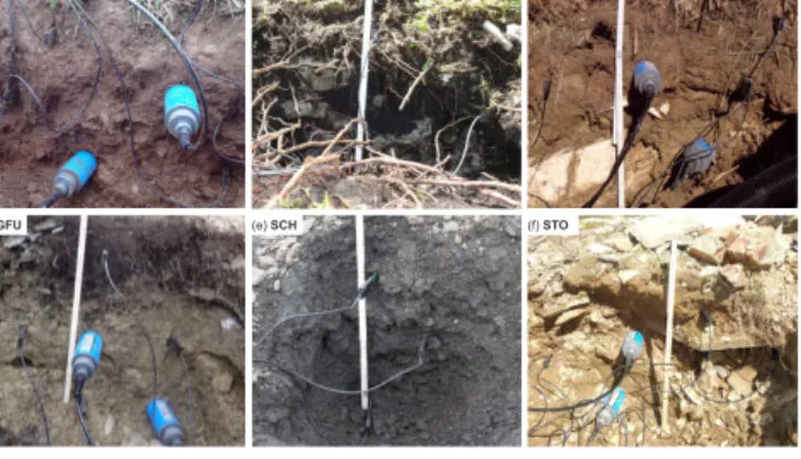
(e) SCH

Figure 3. Illustration of the soil characteristics and sensor installa-tion for all SOMOMOUNT stainstalla-tions.

accuracy of ±6 %vol (Delta-T Devices, 2008; Verhoef et al., 2006). This sensor was selected for its measurement depth and its easy installation. However, it is not suited for hetero-geneous subsurface or coarse-grained material since a good contact between the access tube and the soil is necessary. Fur-thermore, at least 1 m soil is needed for its installation; thus, it was only used at Frétaz (Sect. 2.3).

2.2 Network design

Each soil moisture station is equipped with four to six sen-sors along a vertical profile. The standard instrumentation consists of one SMT100 at 10 cm, two at 30 cm and one at 50 cm as well, as one PICO64 at 30 cm and one at 50 cm (Fig. 2). The doubled sensors at 30 cm were installed to check for long-term instrumental drift. Installation of the complete instrumentation at all depths was not possible at all sites due to soil characteristics. The site-specific set-ups are summa-rized in Table 2.

The same sensor installation procedure was followed at all sites and is based on the criteria described in Krauss et al. (2010) and Mittelbach et al. (2011). While digging the pit for the sensor installation, each soil horizon was stored sep-arately in order to preserve and restore the initial soil profile. At the depth of each sensor, up to two soil samples were col-lected at the side for granulometric analysis and determina-tion of water content. The sensors were then installed in the undisturbed soil with the blade in vertical position to avoid ponding (Figs. 2, 3). Finally, the soil was refilled according to the original order of horizons and compacted to restore its original density. Additionally, larger soil samples (about 8 L) were collected in the vicinity for material-specific cal-ibrations of the sensors (Sect. 3). Data are recorded using a CR1000 data logger (Campbell Scientific) and transmitted wirelessly to an ftp server. The measurement interval is de-pending on the electrical power capacity of each station (see Table 2).

2.3 Field sites

The site selection for the installation of the long-term soil moisture monitoring stations within the SOMOMOUNT project was constrained by the following criteria:

i. sufficiently high elevation, for the ground thermal regime to be affected by seasonally or permanently frozen conditions;

ii. equal distribution along an altitudinal gradient;

iii. availability of additional meteorological data and if pos-sible ground temperature data;

iv. easy access on-site, and a minimum of 50 cm of fine-grained material to guarantee the installation of the sen-sors.

The stations were installed in collaboration with Me-teoSwiss (see SwissMetNet; http://www.meteoswiss.admin. ch) for stations at middle elevation and the Swiss Permafrost Monitoring Network PERMOS (http://www.permos.ch) for stations at higher elevation (see Table 2). Located in the west-ern part of Switzerland, the SOMOMOUNT network covers an elevation range from 1205 to 3410 m a.s.l. with altitudi-nal differences between stations of 400–500 m (Fig. 1). De-tailed information about the climatic conditions and subsur-face properties at each field site are summarized in Table 3. 2.3.1 Frétaz (FRE)

Frétaz is located in the western part of Switzerland on the first crest of the Jura Mountains at an altitude of 1205 m a.s.l. The soil moisture monitoring station is installed within the perimeter of the weather station belonging to the MeteoSwiss automatic network SwissMetNet. In addition, ground tem-peratures down to 1 m depth were measured until 2005.

The surface cover consists of managed grass following the general directives from MeteoSwiss (grass cover maintained at all times at a few cm). The soil is composed of a unique layer of sandy loam down to 50 cm (Table 3). According to geophysical surveys (electrical resistivity tomography, ERT), the limestone bedrock is located at 5 to 10 m depth under-neath the station (see Pellet et al., 2016).

2.3.2 Dreveneuse (DRE)

The Dreveneuse field site is located at an altitude of 1650 m a.s.l. in a small north-orientated valley within the Swiss pre-Alpine region, where the mean annual air temper-ature is around 5◦C (Morard, 2011). The soil moisture sta-tion is installed on a vegetated talus slope near an automatic weather station, and ground temperatures are monitored in two boreholes down to 5 and 14 m depth, respectively.

This site is situated below the lower altitudinal limit of permafrost occurrence in the Alps but is still affected by per-mafrost conditions due to complex air circulation within the

Table 2. Summary of the station instrumentation and characteristics at the field sites Frétaz (FRE), Dreveneuse (DRE), Moléson (MLS), Gemmi (GFU), Schilthorn (SCH) and Stockhorn (STO).

Site Elevation [m a.s.l.] Sensor depth [cm] Measurement interval Start date Related networks

SMT100 PICO64 PR2/6

FRE 1205 10, 30, 30, 50 30, 50 10, 20, 30, 40, 60, 100 10 min 11.10.2013 SwissMetNet

DRE 1650 10, 30, 30, 50 – – 60 min 26.09.2014 PERMOS

MLS 1974 10, 30, 30, 50 30, 50 – 10 min 17.10.2013 SwissMetNet

GFU 2450 10, 30, 30, 50 30, 50 – 30 min 17.07.2013 PERMOS

SCH 2900 10, 30, 50 10 – 30 min 31.07.2014 PERMOS

STO 3410 10, 30, 30, 50 30, 50 – 30 min 27.08.2014 PERMOS

Table 3. Summary of the climatic conditions and soil properties at each SOMOMOUNT station.

Site Elevation T_aira Pa Depth Particle size distribution [%] Textureb Bulk density Organic fraction Thermal regime

[m a.s.l.] [◦C] [mm] [cm] Clay Silt Sand [g cm−3] [%]

FRE 1205 6 1333 0–10 2.2 33.3 52.4 Sandy Loam 0.95 0.1 No frost

10–30 2.5 36.1 39.3 Sandy loam 1.06 –

30–50 3.0 30.8 53.7 Sandy loam 1.01 –

DRE 1650 5 936 0–50 0.6 24.4 71.3 Sandy loam 0.12 7.7 Permafrost

MLS 1974 3 929 0–10 11.8 72.5 15.6 Silty loam 0.58 0.15 Seasonal frost

10–30 15.1 77.6 7.1 Silty loam 0.71 –

GFU 2450 0 1800–2500 0–10 2.0 63.3 34.2 Silty loam 0.58 4.80 Seasonal frost

10–30 2.1 39.7 27.8 Loam 1.52 –

30–50 2.6 46.5 39.8 Sandy loam 1.39 –

SCH 2900 −3 2700 0–10 1.0 14.5 60.0 Loamy Sand 1.53 – Permafrost

10–30 0.6 8.7 40.6 Sand 1.35 –

STO 3400 −5 1500 0–10 0.3 6.4 48.7 Sand 1.42 – Permafrost

10–30 0.6 20.4 56.5 Loamy sand 1.67 –

30–50 0.7 21.6 58.9 Loamy sand 1.54 –

a_{Data source: MeteoSwiss at FRE and MLS; Morard (2011) at DRE; Krummenacher et al. (2008) at GFU; Imhof et al. (2000) and PERMOS at SCH; King (1990) and PERMOS at STO;} b_{According to the USDA classification}

talus slope (Delaloye, 2004). The coarse limestone blocks composing the talus slope are covered by a single layer of organic-rich sandy loam (Table 3, Fig. 3b). The surface is covered by moss and spruces and according to repeated ERT soundings as well as drilling logs, the talus slope is approxi-matively 11 m thick (Morard, 2011).

2.3.3 Moléson (MLS)

The Moléson soil moisture station is situated at 1974 m a.s.l. on top of the eponym mountain in the Swiss pAlpine re-gion. For the reference period 1981 to 2010 the mean annual air temperature was 3◦_{C and the annual sum of precipitation}

is 929 mm yr−1(MeteoSwiss). As for FRE, the soil moisture station is integrated within the perimeter of a SwissMetNet station, where the surface cover consists of managed grass.

No apparent layering was found in the soil profile (homo-geneous layer of silty loam down to 50 cm; see Fig. 3 and Ta-ble 3). According to ERT measurements and the construction journal of the weather station, the bedrock, which consists of

limestone, is located at around 75 cm depth underneath the station.

2.3.4 Gemmi (GFU)

The Gemmi soil moisture monitoring station is located at 2450 m a.s.l. in a west-orientated valley within the main Alpine ridge of Switzerland (Fig. 1). The monitoring station is installed on a solifluction lobe in the direct vicinity of a 1 m deep temperature profile and a weather station (Krum-menacher and Budminger, 1992).

This site is situated just below the lower limit of per-mafrost occurrence in the Alps and therefore undergoes marked seasonal freezing processes down to at least 1 m depth. The surface is covered by grass during the summer and the uppermost 10 cm of the ground is composed of an organic-rich silty loam layer (Table 3, Fig. 3). According to ERT measurements performed in 2014, the bedrock is lo-cated at around 5 m depth underneath the station (Pellet et al., 2016).

2.3.5 Schilthorn (SCH)

The Schilthorn field site is situated at an elevation of 2900 m a.s.l. on a small plateau in the north-facing slope of the Schilthorn summit in the northern Swiss Alps (Fig. 1). The soil moisture station is installed next to an automatic weather station and three boreholes, where ground tempera-tures have been monitored since 1998 (Harris et al., 2001).

Permafrost is present at SCH and the depth of the sea-sonally unfrozen soil layer (the active layer) can reach up to 10 m (PERMOS, 2016). The surface cover is vegetation free and consists of a layer of fine-grained debris with material ranging from loamy sand to sand (Table 3) reaching several metres thickness according to ERT measurements (Hilbich et al., 2008). SCH is the only station of the SOMOMOUNT net-work where soil moisture has already been monitored since end of August 2007 (Hilbich et al., 2011).

2.3.6 Stockhorn (STO)

The highest soil moisture monitoring station of the SOMO-MOUNT network is located at an elevation of 3410 m a.s.l. on the Stockhorn plateau in the western Swiss Alps. The soil moisture station is installed in the vicinity of an automatic weather station as well as two boreholes measuring ground temperatures since summer 2000 (Harris et al., 2001).

The Stockhorn plateau is underlain by at least 100 m deep permafrost (Gruber et al., 2004), where the active layer thick-ness can reach up to 5 m (PERMOS, 2016). The surface is free of vegetation and consists of a 1 m deep layer of fine-grained debris ranging from sand to loamy sand (Table 3) underlain by Albit–Muskovit schist bedrock (Gruber et al., 2004).

2.3.7 Additional stations

In addition to the SOMOMOUNT network, we used the sta-tions of Sion (SIO; Mittelbach and Seneviratne, 2012) and Cervinia (CER; Pellet et al., 2016; Pogliotti et al., 2015) for comparative analysis. The first one is part of the SwissS-MEX network and is located in the Rhone valley at an el-evation of 490 m a.s.l. Since 2009, LSM is measured down to 80 cm depth within the perimeter of the SwissMetNet sta-tion. Conversely, Cervinia is a high-elevation (3100 m a.s.l.) permafrost monitoring site managed by the regional envi-ronmental protection agency of Val d’Aosta (ARPA). Since 2006, the site is equipped with two boreholes (7 and 14 m deep) as well as an automatic weather station and one soil moisture sensor at 20 cm depth.

2.4 Data processing

To ensure the quality of the LSM and ground temperature data, two different automatic filters are applied: a technical filter and a temporal filter. The filters are based on guidelines from Dorigo et al. (2013).

The technical filter is designed to eliminate all unrealis-tic values due to technical issues. First, a threshold method is applied to detect and remove measurements outside of the plausible ranges (< 0 and > 80 %vol for LSM and < −20 and > 30◦C for ground temperature). The threshold for LSM used here was empirically determined based on the data from all SOMOMOUNT stations. It is slightly higher than the 60 %vol proposed by Dorigo et al. (2013) for the In-ternational Soil Moisture Network. Second, the values col-lected with insufficient battery voltage (< 10 V) are removed, since too low power supply can disturb the measurements. For the SMT100 sensors, readings with a raw sensor put (given in moisture counts, MC; see Truebner, 2016) out-side of the laboratory-defined range (MCwater≈9000 and

MCair≈20 000) are also excluded. At all sites the

techni-cal filter eliminated less than 0.1 % of the measured values except at GFU, where the PICO64 sensors had a default in wiring and thus 8.3 % of the measured data had to be ex-cluded.

The temporal filter is designed to eliminate any value ex-hibiting unrealistically large temporal variability (random spikes); 3-day-running means (rmean) and standard

devia-tions (rSD)are calculated for all sensors. Measurement

val-ues lying outside of the range defined by rmean±x · rSDare

subsequently removed, where x is an empirically determined site-specific tolerance factor (3 at FRE and GFU, 4 at DRE, SCH and STO and 5 at MLS). This filter was applied to LSM and ground temperature measurements with an elimination rate varying between 0 % (DRE) and 0.3 % (FRE and SCH) of the measured data.

Numerous data gaps occurred at the different SOMO-MOUNT stations during the monitoring period 2013–2016 (see Fig. 6). They were mainly caused by problems related to power supply (large data gap for all the sensors at a sta-tion, e.g. autumn 2013 at FRE and MLS), data logging (short gaps for all sensors of a station, e.g., winter 2014 at GFU) or sensor malfunction (single sensors for variable time, e.g., PICO64 at 50 cm at the end of summer 2016 at STO). Given the highly variable nature of LSM, no gap filling technique was applied.

2.5 Complementary analysis

All LSM datasets used in the following analysis were homog-enized to hourly arithmetic mean values. For the elevation dependency investigation (Sect. 5.2), annual and seasonal means were calculated for the year 2015, since all stations ex-cept GFU have complete data series during that period. The data gaps at GFU (24 February–1 March 2015 and 24 April– 25 May 2015) were filled for this specific analysis only by linear interpolation between the nearest available data points. Finally, for the analysis of the moisture transport through the ground we used the moisture orbits (see Sect. 5.1).

To analyse and understand the temporal evolution of LSM in detail, additional datasets, such as weather and ground

Table 4. Parameters and statistics of the linear and exponential calibration curve for each station.

Site Linear fit Exponential fit n

a b r2 RMSE [vol.%] c d r2 RMSE [vol.%]

FRE −0.005630 98.15 0.96 2.76 707.1 −0.0002680 0.93 3.66 16 DRE −0.006361 114.7 0.89 5.71 1219 −0.0002889 0.96 3.51 12 MLS −0.008108 139.2 0.97 3.59 741.7 −0.0002507 0.95 5.03 16 GFUmin −0.005327 93.7 0.80 5.57 465.8 −0.0002336 0.75 6.18 13 GFUorg −0.007819 140.2 0.95 3.93 534.2 −0.000209 0.93 4.83 14 SCH −0.004301 77.55 0.81 4.47 899.2 −0.0002925 0.88 3.57 12 STO −0.004851 85.71 0.84 4.02 457.9 −0.0002378 0.79 4.58 18

temperature data, are needed. The stations of SIO, FRE and MLS are located next to SwissMetNet stations and thus datasets with good quality are available. This is not always the case at the high-altitude/permafrost stations DRE, GFU, SCH and STO, where high-altitude-related logistical prob-lems in maintenance lead to data gaps and precipitation is often not measured at all.

For the stations without explicit precipitation measure-ments, precipitation data were extracted from the 2 km grid-ded dataset generated by MeteoSwiss (MeteoSwiss, 2014), which is available at daily resolution and is based on 430 ob-servation stations across Switzerland. Data gaps in the in situ measured air temperature series were completed using the two step quantile mapping approach described in Rajczak et al. (2016). Finally, snow cover duration was extracted from the ground-surface temperature variability using the snow in-dex method described in Staub and Delaloye (2017).

3 Calibration

In order to increase the accuracy of the absolute LSM mea-surements, the SMT100 sensors require a material-specific calibration (Table 4). Using the large soil samples collected at each site, a material-specific calibration was performed in the laboratory following the general procedure outlined by Starr and Paltineanu (2002).

In a first step, the entire soil sample was oven dried and packed into a plastic container at approximatively the field bulk density (see Table 3). A SMT100 sensor was then inserted in the sample and its raw outputs were continu-ously recorded. Finally, a soil sample was collected using a standard 100 cm3 measurement cylinder. In a second step, 200 mL of water was added (LSM increase by about 3– 5 %vol) with subsequent mixing to get a homogenous repar-tition of the water in the calibration sample. The SMT100 was then reinserted, its raw outputs recorded and a soil sam-ple collected. This procedure was repeated until saturation of the soil material was reached, yielding 9 to 12 calibration data points depending on the soil type.

The LSM (θv)of the collected samples was determined

following the standard gravimetric method. For this, the

sam-ples were weighted and oven dried at 105◦C during 24 h for the mineral soils and 60◦C during 48 h for organic soils. The dry samples were then weighted to determine the gravimet-ric water content (mass of water which evaporated θg)and to

calculate the dry bulk density (ρb). Finally, θvwas obtained

using Eq. (1):

θv=ρb·θg (1)

The gravimetric method was also applied to the in situ soil samples collected during the sensor installation. The calcu-lated LSM (θv) values obtained from both the laboratory

and the in situ samples were then fitted to the SMT100 raw data (MC) using a linear (Eq. 2) and an exponential relation (Eq. 3).

θv=a ·MC + b (2)

θv=c · e(MC·d) (3)

Table 4 lists the value of the parameters a, b, c and d for each station, the number of samples considered and the goodness of the fit for both methods. At GFU, two different material-specific calibrations for mineral and organic soil were real-ized due to the clear layering of the soil profile (Fig. 3). At all locations except DRE the linear relation yields higher r2 and lower root mean square error (RMSE) than the exponen-tial relation. Thus, the linear calibration is used for all sites except DRE, where the exponential calibration is used.

For the PICO64, the built-in calibration based on Topp’s equation (Topp et al., 1980) was used and no additional material-specific calibration was performed. In this study the PICO64 sensors are only used for inter-network comparison with the SwissSMEX network but not for further analysis. Thus, for consistency we adopted the same calibration ap-proach as Mittelbach et al. (2011) (i.e. the built-in calibration for generic soils).

Similarly, the manufacturer’s calibration was used for the PR2/6 sensor (Delta-T Devices, 2008), which is mainly used for test purposes within the SOMOMOUNT network. De-pending on the middle-term results further PR2/6 sensors might later be added to the network.

Given the application of the various soil moisture sen-sors at field sites undergoing freezing and thawing processes,

FRE

(a) (b) DRE (c) MLS (d) GFU

FRE

(e) (f) DRE (g) MLS (h) GFU

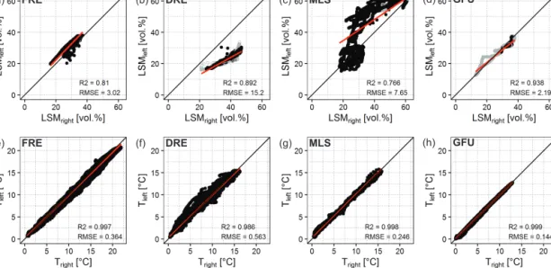
Figure 4. Comparison of measured LSM (upper row) and ground temperature (lower row) from both SMT100 sensors at 30 cm depth using the linear calibration at FRE (a, e), DRE (b, f), MLS (c, g) and GFU (d, h). The hollow grey points represent LSM measurements taken when the ground temperature was below 1◦C.

some considerations are important to make. As mentioned above the frequency based, capacitance and TDR techniques make use of the high permittivity of liquid water (∼ 80) com-pared to the surrounding soil and air (2–9 and 1, respectively) to relate the recorded electromagnetic signal to LSM. How-ever, the permittivity of liquid water is sensitive to temper-ature variations and can increase from ∼ 80 at 20◦C up to ∼88 at 0◦C (e.g. Wraith and Or, 1999), thus introducing an additional uncertainty in the calibration for unfrozen condi-tions. Furthermore, under frozen conditions a part of this to-tal water turns into ice, having again a much lower permittiv-ity (∼ 2–3; e.g. Aragones et al., 2011). Thus, upon freezing, the recorded signal and measured LSM strongly decreases although the total soil moisture stays constant.

Characteristically, at temperatures below 0◦C water and ice can coexist in the soil (e.g. Spaans and Baker, 1995). However, the presented calibration procedure was conducted at room temperature and thus does not account for the pres-ence of ice in the soil mixture. The resulting sensor accu-racy is therefore only valid for above 0◦C ground temper-atures (unfrozen conditions). The use of standard empiri-cal empiri-calibration in frozen conditions often yields overestima-tions of the LSM (e.g. Spaans and Baker, 1995; Yoshikawa and Overduin, 2005). For frozen sand, however, Watanabe and Wake (2009) showed that TDR devices calibrated using Topp’s equation exhibit only small deviations from the mea-sured LSM using nuclear magnetic resonance (NMR) except at temperatures between 0 and −1◦C.

Although the absolute accuracy of measured LSM under frozen conditions is difficult to assess, its relative changes are well captured. At SCH, Hilbich et al. (2011) showed that the soil apparent resistivity (using data from continuous ERT

monitoring) and LSM (measured with the precursor model of the SMT100) exhibit consistent variations under frozen and unfrozen conditions. Given the sandy composition of the ground at SCH and STO, as well as the evidence from the co-inciding resistivity measurements (see also Hauck, 2002), we find the LSM data with standard calibration to be consistent enough for further analysis. Given the generally lower accu-racy of the soil moisture sensors under partially frozen and frozen conditions, the LSM measurements carried out at tem-peratures below 1◦_{C are clearly identified in all figures}

here-after. The 1◦_{C threshold was selected to account for partially}

frozen conditions as well as the scale mismatch between the temperature and LSM measurements. These data have thus to be interpreted with care, especially regarding their absolute values.

4 Results

4.1 Sensor comparison and consistency

At 30 cm depth two SMT100 sensors have been installed in parallel to investigate potential instrumental drift over longer time periods. Comparing their outputs also allows us to as-sess the quality of the sensor installation, the reliability of the measurements and potential spatial heterogeneity.

At FRE, DRE, MLS and GFU the correlation between the LSM measured by the two sensors is found to be satisfactory (lowest correlation at MLS: r2=0.766, Fig. 4). The RMSE is more variable with the lowest value at GFU (2.19 %vol) and the largest at DRE (15.2 %vol). Deviations from the one-to-one correspondence of the two sensors (black line in Fig. 4) can be attributed to small-scale soil heterogeneities

Figure 5. Comparison between PICO64-measured (x axis) and SMT100-measured LSM (y axis) at all sites. The linear relation is used for the SMT100 calibration. The hollow grey points at GFU, SCH and STO represent measurements taken when the ground temperature was below 1◦C.

surrounding the sensors. Soil heterogeneities can result in differences of reaction time to infiltration and/or evapora-tion events as well as wet or dry biases due to different soil properties. This is particularly visible at MLS, where an in-crease of LSM is systematically recorded first by the left sen-sor (y axis) and later by the right sensen-sor (x axis). At DRE (Fig. 4b) the right sensor shows consistently higher values (∼ 5–10 %vol) than the left sensor, but the relation between the measured LSM values is almost constant, illustrating the effect of different soil properties.

DRE is also the site with the largest RMSE (0.563◦C) be-tween the measured temperatures at 30 cm depth, indicating that specific physical processes such as convective heat trans-port through airflow within the coarse blocks of the ground (e.g. Wicky and Hauck, 2017) may influence the two sensors in a different way (see Sect. 5.3). At FRE, MLS and GFU the measured temperatures correspond almost perfectly one-to-one showing no different physical processes. Therefore, the LSM deviations are most likely due to soil heterogeneities.

Sensor comparison was only possible at four sites. At SCH the terrain prevented the installation of two sensors at 30 cm, whereas at STO one of the installed sensors gives unreliable data. This sensor probably suffers from bad coupling with the soil (air pockets near the blade and thus bad contact with the soil) stemming from a faulty installation due to the blocky subsurface.

In addition, the TDR-based PICO64 sensors, having a nominally higher absolute accuracy (Mittelbach et al., 2012), have been installed at 30 cm depth. Similar to Fig. 4, the com-parison between SMT100 and PICO64 sensors at the same

depth shows a generally good correlation (lowest r2=0.542 at STO) with some deviations from the one-to-one relation (Fig. 5). The RMSE is generally larger than for the SMT100 intercomparison (Fig. 4) at all sites, which can be explained by the different measurement volume of the SMT100 and PICO64 sensors (see Sect. 2.1 and Fig. 2). At FRE and GFU the comparison between PICO64 and SMT100 LSM mea-surements yields very similar results to the comparison of the two SMT100 sensors, with slightly higher RMSE values (4.53 and 2.53 %vol, respectively). MLS shows a larger dy-namic range and mostly higher values for the SMT100 sen-sor (RMSE = 16.1 %vol), but a similar temporal variability (r2=0.641). A similar pattern is observed, when comparing the PICO64 sensor with the second SMT100 sensor installed at 30 cm (Table 5). This dry bias of the PICO64 sensor at MLS is probably due to a bad contact between its rods and the surrounding soil. At SCH and STO the differences be-tween the sensors have a characteristic shape, but are centred on the one-to-one relation. It can be attributed to different on-set of freezing and thawing at the two sensor locations (see also Fig. 6e–f). In addition, clear wet and dry biases in the PICO64 measurements are observed at SCH and STO, re-spectively, which can be explained by an unreliable calibra-tion using Topp’s equacalibra-tion for the high-mountain subsurface material present at SCH and STO (e.g. Robinson, 2004).

Figure 5 only considers the sensors at 30 cm (left) at all sites with the exception of SCH, where the 10 cm sensor is used, since it is the depth of the only available PICO64. The same analysis was performed with the 30 cm right and 50 cm sensors (Table 5). The overall results are very similar

regard-Figure 6. SMT100 measured LSM (upper panel) and ground temperatures (lower panel) at each SOMOMOUNT station (a–f). At FRE the uppermost panel displays the PR2/6 measured LSM. The vertical dotted lines at FRE and SCH indicate the period analysed in Fig. 7. The dashed LSM lines represent the soil moisture measurements taken when the ground temperature was below 1◦C.

Table 5. Correlation (r2)and RMSE between the PICO64 and SMT100 measured LSM at all sites.

Site 10 cm 30 cm left 30 cm right 50 cm

r2 RMSE [vol.%] r2 RMSE [vol.%] r2 RMSE [vol.%] r2 RMSE [vol.%]

FRE – – 0.830 4.53 0.934 2.12 0.504 10.4

MLS – – 0.641 16.1 0.848 12.1 0.553 10.1

GFU – – 0.959 2.53 0.890 2.37 0.910 1.78

SCH 0.811 7.56 – – – – – –

STO – – 0.542 4.18 – – 0.807 6.93

ing statistical fit (lowest fit at MLS and highest fit at GFU) and observed patterns (not shown).

4.2 Soil moisture temporal evolution

Figure 6 shows the evolution of LSM and ground tempera-ture at all SOMOMOUNT stations from July 2013 until

Au-gust 2016. The temperatures exhibit a typical seasonal pat-tern with maximum values during the summer and minimum values in winter. The amplitude of these seasonal variations is specific to each site. DRE, GFU, SCH and STO exhibit tem-peratures close to and below the freezing point during the winter, whereas no freezing was recorded at FRE. At MLS

10 cm 30 cm left 50 cm

Soil moisture: Soil temperature: A

10 cm 30 cm left 50 cm Snow depth tmospheric forcing: S Air temperature Precipitation LSM [vol.%] Snow depth [cm] Precipitation [mm d ] -1

April May June July August 2015: March

Temperature [°C]

Unfrozen Frozen Zero-curtain Unfrozen

Snow depth [cm] Precipitation [mm d ] -1 Temperature [°C] Specific resistivity [Ωm] (a) FRE (b) SCH

April May June July August 2015: March A B oil resistivity: 19 cm 56 cm 94 cm LSM [vol.%] 40 20 60 0

Figure 7. SMT100 measured LSM, ground temperature and soil resistivity at FRE (a) and SCH (b) from March to August 2015. In addition, daily air temperature, snow depth and precipitation sums are shown as well as the date of the transition between the different stages in the thermal evolution at SCH at 10 cm (dashed lines A and B; see text for details). The dashed LSM lines represent the soil moisture measurements taken when the ground temperature was below 1◦C.

negative soil temperatures were only observed at 10 cm depth during 10 days in early winter 2016.

On the other hand, the LSM differs strongly at each station and no common pattern is found. The sites can be divided into two categories of LSM dynamics: a low-elevation pat-tern at FRE and MLS characterized by a summer minimum of short duration and high LSM values for the rest of the year. The second category, typical for high elevations (SCH and STO), is defined by a long-lasting LSM minimum in win-ter, and maximum absolute values accompanied by strong variability during the summer. GFU and DRE display fea-tures characteristic from both categories, namely a long win-ter minimum as well as LSM decrease during summer. At GFU the 10 cm sensor values are much more variable than the values at 30 and 50 cm and exhibit higher values. This is due to the high organic content and low bulk density of this particular soil layer (Fig. 3d and Table 3).

Comparing the two summer seasons in 2014 and 2015 at FRE, MLS and GFU, one can observe a stronger LSM de-crease in 2015 at all sites. This marked LSM dede-crease is due to the exceptionally high air temperatures and low precipi-tation recorded in July 2015 (MeteoSwiss, 2016; Scherrer et al., 2016), leading to increased evaporation. However, the ef-fect of this anomalous event on LSM is different at all sites. At MLS the effect is the most pronounced (44 %vol LSM loss at 30 cm) and the LSM in the uppermost layers have still not returned to their original values in May 2016. At FRE the effect is less marked (18 %vol LSM loss at 30 cm) and

shorter but it can be observed down to 100 cm. At DRE a drying is seen at all depths with a similar amplitude (12 %vol LSM loss at 30 cm), whereas at GFU the effect is strong but of short duration at 10 cm (40 %vol LSM loss) and almost not seen below. Finally, at the two highest stations (SCH and STO) no characteristic LSM decrease is observed.

To characterize these two patterns of LSM dynamics iden-tified above in more detail and to analyse the processes con-trolling them, we focus on a 5-month period from spring to summer 2015 at FRE and SCH (Fig. 7).

At FRE the minimum LSM is reached during the summer, when air temperatures are highest and thus evaporation is maximal. No clear LSM maximum can be identified through-out the year (Fig. 6a) but multiple maxima are observed fol-lowing precipitation events. The snow cover, which disap-peared mid-March in 2015, reduces the link between LSM variations and atmospheric conditions. During the snowmelt period only a small LSM increase is seen, which could be at-tributed to conditions close to saturation throughout the win-ter. After the disappearance of the snow cover the variability of LSM increases at all depths and is systematically related to precipitation events (LSM increase) and dry spells, both, with and without air temperature increases (LSM decrease). As expected, the uppermost layer (10 cm) reacts stronger to atmospheric forcing than layers below. However, the re-sponse time is very fast and in some cases almost simultane-ous at all depths, which is an indication for preferential flow.

At SCH the evolution is very different. Minimum LSM values are recorded in winter, when the ground is entirely frozen and the maximum is reached in early summer due to the combined effect of snowmelt and thawing of the ground (Figs. 6f, 7b). As long as ground temperatures are below the freezing point, the meltwater from the snow cover is either running off directly at the surface or refreezes at the top of the frozen layer (and releases latent heat which can contribute to further thawing; e.g. Scherler et al., 2010). In contrast to FRE (Fig. 7a), the evolution of LSM at SCH is mainly driven by ground temperatures and the snow conditions and it is less affected by liquid precipitation. Three main stages of LSM evolution and ground thermal regime can be identified. The frozen stage is characterized by the lowest LSM values due to the frozen state of the ground and the insulating snow cover. It is followed by the zero-curtain period, defined by Outcalt et al. (1990) as extended period of time with near 0◦_{C temperature induced by latent heat effects in a}

thaw-ing or refreezthaw-ing active layer. Durthaw-ing this period LSM in-creases/decreases slowly but remains decoupled from precip-itation events. Punctual lateral inflow and/or snowmelt water infiltration are possible (see Hilbich et al., 2011). Finally, the unfrozen stage coincides with the snow-free period and is characterized by high LSM variability coupled with the pre-cipitation events. Although, the accuracy of the LSM mea-surements during the frozen and zero-curtain periods is diffi-cult to assess due to the presence of ice, the relative changes, and thus the timing of each phase, are well captured. The LSM variations are coherent with the change of specific re-sistivity in the uppermost ∼ 50 cm of the ground. Similar to the dielectric permittivity, the electrical resistivity is highly dependent on the amount of unfrozen water content in the ground (Hauck, 2002). The frozen stage is thus character-ized by high resistivities and a marked drop is observed dur-ing the zero-curtain period due to the thawdur-ing of the ground (see also Hilbich et al., 2011). Finally, the unfrozen stage ex-hibits the lowest resistivity values. The same typical stages of LSM evolution have been described for other mountain permafrost sites (e.g. Pellet et al., 2016) and landforms (e.g. Zhou et al., 2015). These stages are also observed in the data collected by spatially distributed SMT100 sensors installed at 30 cm depth at SCH and STO, with marked differences in absolute LSM as well as variable onset and duration of the three stages even at close vicinity (not shown).

5 Discussion

5.1 Dominant processes

To visualize how the moisture is transported through the ground we adapted the thermal orbits (Beltrami, 1996) to LSM (moisture orbits). It consists of a scatter plot of simulta-neously measured LSM at two different depths. The shape of the resulting point cloud depends on the nature and speed of

the vertical transport of water through the soil layers, as well as on soil properties such as hydraulic conductivity, degree of saturation and porosity. Using moisture orbits of differ-ent timescales (annual, pluri-annual and evdiffer-ent), allows us to analyse the dominant processes for the temporal evolution of LSM.

5.1.1 Seasonal variations

To investigate the seasonal dynamic of LSM, we used mois-ture orbits between the SMT100 sensors installed at 10 and 50 cm depth for the year 2015 at each site (Fig. 8). Again, the field sites can be divided in two categories of LSM dynamics, controlled by different processes.

FRE and MLS exhibit similar moisture orbit shapes driven by precipitation events and evaporation. They are divided into three main stages. From January to May the LSM is maximal at both sensors, with some small variations due to snowmelt and/or precipitation events. Starting in June, the summer evaporation causes the LSM to decrease strongly at 10 cm and slightly at 50 cm. Then LSM simultaneously de-creases at both depths due to the increased evaporation gen-erated by the July 2015 heat wave. Finally, LSM increases again, with different speed at each depth. The main differ-ence between the two stations is that at MLS the orbit is not closed. At the end of 2015 there is about 30 %vol LSM less than at the beginning of the year. It indicates that at MLS the near-surface LSM did not recover from the increased evapo-ration generated by the heat wave in July 2015 (see Fig. 6). The dry top soil conditions can generate a large water po-tential gradient with depth and thereby an increased infiltra-tion capacity, but also suitable condiinfiltra-tions for potential pref-erential flow processes, which tend to induce bypass flow of precipitation water (e.g. Wiekenkamp et al., 2016). On the contrary, at FRE the LSM returned to its original value. Both sites received a similar amount of precipitation following the heat wave, from July to end of 2015 (443 and 534 mm, re-spectively, MeteoSwiss). Furthermore, the atmospheric forc-ing (i.e. air temperature, radiation and calculated potential evaporation) was very similar as well (MeteoSwiss). There-fore, the larger and longer-lasting impact of the 2015 heat wave at MLS is due to the higher initial LSM and thus lower potential evaporation limitation than at FRE. The amount of available water for evaporation is dependent on the soil prop-erties. At MLS the soil type is silty loam and is able to retain more water than the sandy loam present at FRE.

At SCH and STO the shape of the moisture orbit is con-trolled by freezing/thawing processes. It can be divided into five stages consistent with the frozen, zero-curtain and un-frozen state of the ground. At the beginning of the year both sensors show their lowest value (frozen stage). This is fol-lowed by a sharp increase at 50 cm not seen at 10 cm (1) and a strong increase at 10 cm but not at 50 cm (2) consistent with the melting of the ground from underneath, which takes place at different times at the two depths (spring zero

cur-FRE DRE MLS SCH GFU (a) (d) (e) (b) (c) STO (f) 1 2 3 1 2 1 2 4 3 5 1 3 4 5 3 Date 2015-04-10 2015-07-19 2015-10-27 2

Figure 8. Moisture orbit at each SOMOMOUNT station from the 1 January to the 31 December 2015. The numbered arrows indicate the most important stages at each station as well as the sense of the evolution. The hollow circles represent LSM measurements taken when the temperature was below 1◦C at 10 cm.

tain). The start of the thawing process at larger depth can be due to preferential water infiltration events or to the influ-ence of high temperatures from the preceding summer (e.g. Zenklusen Mutter and Phillips, 2012). In the latter case, the ground temperatures in spring are higher at depth compared to the near surface due to the time lag of heat propagation into the subsurface. The occurrence of this phenomenon de-pends on the thermal properties of the subsurface and the strength of the winter freezing. Although the thawing process systematically starts at the surface in response to meteorolog-ical forcing, the heat reservoir remaining at larger depth can also start the thawing from below. This process is more likely to occur where the permafrost temperatures are close to 0◦C as it is the case at SCH. During the summer, the ground is un-frozen and strong variations are recorded at both depths (3). The orbit is finally closed by a succession of LSM decrease at 10 cm not seen at 50 cm (4) and a strong decrease at 50 cm but not 10 cm (5), consistent with the downward propagation of the freezing front from the surface (autumn zero curtain). The orbits are closed at both sites indicating no long-lasting perturbation during the year 2015 as well as similar winter conditions. These stages have also been observed by, e.g., Hilbich et al. (2011) and Zhou et al. (2015).

At DRE and GFU it is difficult to determine a clear tem-poral evolution of LSM. DRE exhibits a winter and summer minimum (see also Fig. 6b) corresponding to the freezing of the ground and the summer evaporation peak, respectively.

This double minimum is also found at GFU but less marked, especially at the deeper layer.

5.1.2 Soil type dependency

At DRE the shape of the moisture orbit is almost diago-nal indicating very rapid transfer of water from the surface downward and little storage in the uppermost soil layer (wet anomaly at 50 cm). This is due to the soil properties. At DRE the soil profile down to 50 cm consists of one single organic-rich sandy loam layer with a very low bulk density (Table 3), which is underlain by large sized boulders. These particu-lar soil properties render the uppermost layer highly drain-ing (Berdrain-inger et al., 2001) and the water is rapidly trans-ported through. The boulders underneath do not retain the water, likely preventing the creation of any shallow water ta-ble. Furthermore, and in contrast to the large blocks below, the organic-rich material at the surface retains the water and has a larger thermal conductivity (Beringer et al., 2001), thus favouring summer evaporation and winter freezing.

At GFU the presence of an organic-rich layer in the upper-most 10 cm of the soil causes the measured LSM at 10 cm to be highly variable and generally higher than in the remaining soil column (see also Fig. 6d). At 50 cm the measured LSM shows near-saturation conditions throughout the year indicat-ing a potential influence of shallow groundwater. This is con-firmed by additional ERT measurements realized in summer

from 2013 to 2015, which indicate extremely low specific re-sistivities (∼ 250  m) down to 2.5 m (not shown). The com-bination of these two factors explains the almost horizontal moisture orbit shape observed at GFU. The organic-rich layer has a lower thermal conductivity (Beringer et al., 2001) than the other soil types, thus reducing the influence of air tem-perature (evaporation and/or freezing) at larger depth. Fur-thermore, at 30 and 50 cm the soil is composed of loam and sandy loam with much larger bulk densities (Table 3), which are typically characterized by lower hydraulic conductivities if no preferential flow is occurring (Cosby et al., 1984). These soil properties also contribute to the observed lower LSM variability at these depths.

At FRE and MLS, the soil type is relatively homogeneous within the uppermost 50 cm of the ground, which results in similar LSM temporal evolution with only slight variations in timing and absolute values between the sensors. At MLS the soil type is silty loam and is thus able to retain more water than the sandy loam present at FRE. Finally at SCH and STO, the ground consists of sand or loamy sand, with a significant proportion of soil particles larger than 10 mm (25 and 45 %, respectively, at 10 cm; see also Fig. 3e–f). Such soil com-position is highly heterogeneous even over small distances explaining the high variability between the sensors as well as the comparatively low LSM during unfrozen and snow-free periods.

5.1.3 Climate dependency

As seen in Fig. 6, the LSM temporal evolution is strongly in-fluenced by the variations in atmospheric conditions such as the heat wave of July 2015. Thus, the shapes of the moisture orbits can be different for each year even though the same processes are dominant (evaporation or freezing). Compar-ing all years where measurements are available (Fig. 9), one can see that at low elevation (FRE), where the evolution of LSM is mainly controlled by evaporation and precipitation, the moisture orbits of the year 2014 and 2016 are very sim-ilar in shape and amplitude, whereas 2015 is marked by an exceptional decrease of LSM at both depths.

Conversely, at high elevation in permafrost terrain (SCH), 2015 is not particularly anomalous and the same patterns with comparable amplitudes are observed in all years avail-able. This is to be expected since the freezing/thawing pro-cesses occur every year, with only slight variations regarding snow duration and timing.

Finally, at GFU, which is an intermediate site with sim-ilar characteristics to both FRE and SCH, two very differ-ent orbit shapes can be observed. In 2014, the ground froze down to 50 cm producing a moisture orbit similar to SCH and STO characterized by large variations occurring at the two sensors. Conversely, in 2015 and 2016 only the 10 cm layer froze, yielding horizontal shaped moisture orbits.

5.1.4 Infiltration events

Using differential moisture orbits one can also characterize single infiltration events and investigate further the influence of the soil type on the short-term LSM evolution. We selected one precipitation event recorded at all six stations and plot-ted the moisture orbits for a period of 5 days (Fig. 10). At all sites except STO, this precipitation event yields clear mois-ture orbits of different shapes and amplitudes. The slope of the orbits indicates at which depth the LSM is most affected by the precipitation event and the amount of infiltrating wa-ter.

At FRE, GFU and SCH the orbits are horizontal (SCH) to slightly inclined (FRE and GFU), showing that the strongest variations of LSM are occurring at 10 cm. The wetting and drying phases are faster and the perturbation is larger at 10 cm than at 50 cm. At SCH the maximum LSM at 10 cm is reached after 2 h while no variation is recorded at 50 cm during that interval. The LSM starts increasing at 50 cm once the LSM at 10 cm is already decreasing. This pattern is con-sistent with the vertical succession of soil material found at SCH: sandy loam near the soil surface, which retains water at the beginning of the event and sand at larger depth, which is more draining. At FRE and GFU the orbits correspond to soils with smaller hydraulic conductivity and higher re-tention capacity (sandy loam and loam–sandy loam, respec-tively, Table 3).

At DRE the moisture orbit has a large amplitude at both depths with a slope > 45◦. It indicates a rapid transfer of wa-ter through the soil and little storage at 10 cm, which is typ-ical for the particular soil composition found at DRE (single organic-rich layer with low bulk density underlain by coarse blocks with large interconnected pores).

At MLS the moisture orbit is almost vertical due to LSM increase/decrease at 50 cm depth only, which indi-cates an instantaneous transfer of water through the upper-most layer. It is the station where the event was the small-est (+8 mm d−1)but the resulting perturbation was the sec-ond highest (> +7 %vol). From Fig. 6c, it can be seen that, at the time of the precipitation event, the LSM at 10 and 30 cm depths were unusually low (23 and 24.5 %vol, respec-tively), thus generating a larger gradient in pressure head from the surface to the lower soil layers as well as provid-ing very suitable conditions for the activation of preferential flow (see, e.g., Wiekenkamp et al., 2016). The degree of sat-uration of the soil layer is thus another key factor influencing the LSM dynamics. The almost total absence of LSM varia-tion at 10 cm during this infiltravaria-tion event could also indicate lateral flow of water.

Our interpretation of the moisture orbit shapes accounts only for vertical transfer of water in the soil. However, lateral flows can also play an important role. At DRE, MLS, SCH and STO the stations are located on slightly inclined slopes or at their bottom. Furthermore, permanent snow patches have been observed at SCH and STO on several occasions and

FRE: no frost

(a) (b) GFU: seasonal frost (c) SCH: permafrost

2014 2013 2015 2016 2014 2013 2015 2016 2014 2013 2015 2016

Figure 9. Moisture orbits at FRE (a), GFU (b) and SCH (c) for the consecutive monitoring years (January 2014–August 2016 at FRE, August 2013–August 2016 at GFU and August 2014–June 2016 at SCH). The hollow circles represent LSM measurements taken when the temperature was below 1◦C at 10 cm.

FRE DRE MLS SCH GFU (a) (d) (e) (b) (c) STO (e) + 27 mm d-1 + 35 mm d-1 _{+ 8 mm d}-1 + 17 mm d-1 _{+ 13 mm d}-1 _{+ 16 mm d}-1 2015-08-23 2015-08-24 2015-08-25 2015-08-26 2015-08-27

Figure 10. Moisture orbit at each SOMOMOUNT station for one precipitation event between the 23 and the 27 August 2015. The LSM values are given as hourly mean and expressed as the change of absolute value compared to the first measurement (23 August at 23:00). The daily precipitation sums recorded (FRE, DRE and MLS) and extrapolated (GFU, SCH and STO) for the 24 August are indicated.

may constitute a continuous water supply during summer (Python, 2015; Wicki, 2015). The infiltration of snowmelt water is a spatially very heterogeneous process on slopes, especially when the subsurface is characterized by large size particles and draining soil types. An example of the influence of snowmelt processes can be seen at STO, where the precip-itation event shown in Fig. 10e did not yield a clear moisture orbit. Its effect is lost in the daily moisture orbit patterns due to snowmelt cycles. For each day shown in Fig. 10e, an oval shaped moisture orbit is present. These daily cycle orbits are very similar in amplitude and structure. The uppermost sen-sor reacts first (wetting and drying) and the maximum LSM increase happens at the same time at both depths.

As seen above for MLS, the influence of a single precipita-tion event on LSM depends not only on the soil properties but also on the moisture conditions prior to the event. To investi-gate this process we computed the moisture orbits of three se-lected precipitation events at FRE and DRE, which were pre-ceded by different LSM conditions (Fig. 11). The first event in mid-May is a combination of low precipitation amount preceded by comparatively high LSM. The second event is of very different amplitude at both sites (+39 mm d−1at FRE and +10 m d−1at DRE) but it marked the end of the summer 2015 heat wave at both sites. The last event is the same as in Fig. 10. It consists of a large amount of precipitation pre-ceded by relatively high LSM.

FRE (b) 30 cm left 30 cm right 50 cm 10 cm Precip (a) DRE 1 2 3 2015-08-24 2015-08-25 2015-08-26 2015-08-27 2015-08-23 + 27 mm 2015-07-18 2015-07-19 2015-07-20 2015-07-21 2015-07-17 + 39 mm 2015-05-16 2015-05-17 2015-05-18 2015-05-15 + 11 mm 2 3 1 2015-08-24 2015-08-25 2015-08-26 2015-08-27 2015-08-23 + 35 mm 2015-07-18 2015-07-19 2015-07-20 2015-07-21 2015-07-17 + 10 mm 2015-05-15 2015-05-16 2015-05-17 2015-05-14 + 13 mm 2015-05-18 3 3 2 2 1 1

Apr May Jun Jul Aug Sep Oct

Apr May Jun Jul Aug Sep Oct 30 cm left 30 cm right 50 cm 10 cm Precip LSM [vol.%] Precipitation [mm d ] -1 LSM [vol.%] Precipitation [mm d ] -1

Figure 11. Moisture orbit at FRE (a) and DRE (b) for three precipitation events in 2015. The LSM values are hourly means and expressed as the change of absolute value compared to the first measurement (first day at 23:00). The daily precipitation sums recorded at the beginning of each event are indicated.

At FRE, the first and third events yield similar moisture or-bit shapes with a larger amplitude for the larger precipitation event. However, the second event produces a diagonal mois-ture orbit with almost no LSM decrease. As for MLS above, the LSM is low at all depths creating suitable conditions for preferential flow as well as an increased infiltration capac-ity due to a high gradient of water potential. Both processes could explain the larger and faster increase of LSM observed at larger depth due to the bypass of the dry uppermost layer. The same indications for preferential flow are seen at DRE, where the second precipitation event is comparatively small (+10 mm d−1)but yields the strongest and fastest LSM in-crease at depth. Given the soil properties, the preferential flow interpretation is preferred to the enhanced infiltration capacity.

5.2 Altitude dependency

As seen above four main processes are driving the annual LSM dynamics, namely evaporation/infiltration and freez-ing/thawing of the ground. The respective predominance of one of these processes is dependent on the station location and more specifically on its elevation. Using all SOMO-MOUNT stations as well as selected SwissSMEX stations (SIO, PAY and PLA) and Cervinia, we investigated the ele-vation dependency of mean annual and mean seasonal LSM for the year 2015 (Fig. 12a).

The relation between LSM and elevation is clearly non-linear. Disregarding DRE (see Sect. 5.3), a distinct pattern emerges. The mean annual LSM regularly increases with el-evation until about 2000 m a.s.l. and then decreases with in-creasing elevation. This tipping point corresponds also to a

clear shift in the LSM regime. Below 2000 m a.s.l. the max-imum LSM is recorded in winter and the minmax-imum in sum-mer, whereas above this threshold the inverse occurs (maxi-mum LSM in summer and mini(maxi-mum in winter).

This shift in LSM regime can be related to a series of vari-ables, which are known to be important for mountain cli-mates and which have also been plotted against elevation (Fig. 12b–e). Air temperature (Fig. 12b) is one of the control-ling factors for evaporation and freezing processes, whereas the precipitation amount (Fig. 12c) controls the water input at the surface. Snow cover duration (Fig. 12e) has several effects on the LSM dynamics: it insulates the ground from the cold winter temperatures (yielding positive surface off-sets, i.e. the difference between ground and air temperature; Fig. 12b) and it acts as a water retention layer, which stores water throughout winter and liberates it in spring/early sum-mer. For each variable, all available data from the monitor-ing networks of MeteoSwiss, PERMOS and IMIS (Intercan-tonal Measurement and Information System maintained by the SLF) were collected and a linear regression model was calculated based on the annual mean (resp. sum) of the year 2015. Globally, the same elevation dependency trends are ob-served using the single stations (dots) or the entire datasets (regression lines).

From Fig. 12 the following relationships can be deter-mined: ground and air temperature, as well as the thaw-ing degree days (absolute sum of positive temperatures per year) all linearly decrease with elevation, yielding a decreas-ing trend of evaporation and thus a theoretically increasdecreas-ing trend of LSM. Conversely, the freezing degree days (ab-solute sum of negative temperatures per year), surface off-set and the snow cover duration increase with elevation,

Figure 12. Elevation dependency of the winter, summer and annual mean LSM at 30 cm depth (a), air, ground temperature and surface offset (ground minus air temperature) at 10 cm (b), annual precipitation sum including selected SwissMetNet stations for comparison (see Fig. 1) (c), freezing and thawing degree days (calculated from ground temperatures at 10 cm) (d) and snow duration (calculated from ground temperature at 10 cm using the method described in Staub and Delaloye, 2017) (e) during the year 2015. The LSM values for SIO, PAY and PLA are part of the SwissSMEX network (Mittelbach and Seneviratne, 2012). Due to missing data at 30 cm, the LSM shown for PAY and PLA was measured at 50 and 20 cm at CER. The dashed green lines illustrate the linear regression based on all available SwissMetNet, PERMOS and IMIS stations in Switzerland (the numbers of station with complete data series in 2015 are indicated) and the shaded areas represent the 99 % confidence intervals. The length of each regression line corresponds to the maximum elevation of the available stations.

which results in longer-lasting winter LSM minimum and thus lower mean annual LSM with increasing elevation. Fi-nally, a slightly increasing trend in the precipitation distribu-tion is observed with large site-specific variadistribu-tions due to the strong microclimatic effects; however, on larger spatial scale (continental) precipitation is known to increase with eleva-tion (Smith, 1979). This combinaeleva-tion of overall increasing precipitation and decreasing evaporation yields a trend of in-creasing LSM with elevation until the altitude threshold of about 2000 m a.s.l., where it is balanced by the increasingly important ground freezing. Above this threshold LSM starts decreasing with elevation.

At lower elevation (below 2000 m a.s.l.), evaporation dom-inates the LSM regime, causing the summer LSM minimum. With increasing elevation air temperature decreases, precip-itation increases and the snow cover duration is prolonged, explaining the increase of mean annual LSM.

At higher elevation (above 2000 m a.s.l.), the ground ther-mal regime and more specifically the soil freezing process drives the LSM regime, causing the LSM minimum to shift from summer to winter, when freezing occurs. This is con-firmed by the observed negative ground temperatures as well as the increasing freezing degree days. Air and ground temperatures decrease with increasing elevation yielding in-creasingly long duration of seasonally frozen ground and thus explaining the decreasing trend of LSM.

5.3 Special case: Dreveneuse

To summarize the findings from the SOMOMOUNT network presented above, a simple theoretical model of the distribu-tion of LSM and its contributing factors with elevadistribu-tion can be visualized with the grey shading in Fig. 13. Comparing the observations qualitatively with this model (circles in Fig. 13),

Tground

P

Tair

Snow

LSM

SIO FRE DRE MLS GFU SCH STO

492 1205 1650 1974 2450 2900 3400 Elevation [m a.s.l.] Warm Wet High Cold Dry Low Theoretical evolution: Observations: Warm Wet High Cold Dry Low Soil type: Silty loam Loam Sandy loam Sand

Figure 13. Generalized schematics of the evolution of air temper-ature, precipitation, snow duration, ground temperature and LSM with elevation. The circles represent the observations from 2015 (see Fig. 12), the grey area the expected theoretical evolution and the colour scale the soil type. The mismatches between model and observations are highlighted in red.

it can be seen that DRE does not fit the model. The recorded mean annual LSM values are much lower than expected. This is due to the composition of the soil profile, which is an elevation-independent factor. The uppermost layer of the subsurface has a very high porosity (> 90 %, see Table 3), which leads to exfiltration of water into the underlying talus slope or lateral water transport. Furthermore, and conversely to FRE and MLS, no evidences of groundwater influence are seen at DRE (Fig. 6). This is consistent with the coarse blocky structure of the talus slope, which does not retain the infiltrating water.

The case of DRE is also particular in terms of snow dura-tion (longer than expected) and mean annual ground temper-ature (lower than expected). Both anomalies are due to site-specific characteristics, which are independent from eleva-tion. The low mean annual ground temperature results from convective heat transport by a complex air circulation within the underlying talus slope (Delaloye, 2004; Morard, 2011), which is made possible by the large interconnected pore space between the coarse blocks of the talus. During winter, ascending warm air within the talus slope leads to cold air in-flow at the bottom of the talus slope, where the soil moisture and weather stations are located. This process is able to effi-ciently cool the ground even when the snow cover is present. In summer the air circulation is reversed and a gravity-driven outflow of cold air from the inside of the talus slope takes place at the bottom, where LSM and ground temperatures are measured. This process has been observed at many sim-ilar talus slopes in low and high-elevation mountain regions (e.g. Delaloye and Lambiel, 2005; Gude et al., 2003; Kneisel et al., 2000; Sawada et al., 2003; Wakonigg, 1996). Further-more, the lower ground temperatures caused by the air

cir-culation have been successfully reproduced using numerical modelling (Wicky and Hauck, 2017). The longer snow dura-tion is due to the spruces and low vegetadura-tion surrounding the station, which efficiently traps the snow for an extended pe-riod of time. The cold ground temperatures help in addition to conserve the snow cover for a longer period.

The relatively low elevation of DRE implies a high air tem-perature and thus more energy available for evapotranspira-tion. Additionally, the presence of vegetation at the surface induces water uptake. The reduced ground temperatures by the air circulation result in a negative surface offset (ground temperature lower than air temperature) and slightly positive freezing degree days, both indicating a seasonal freezing of the ground. Thus, two phases of minimal LSM values are ob-served: one during the summer due to evaporation and one in winter due to partial or complete freezing of the ground (see Figs. 6b, 12a).

The elevation-dependent generalized schematics shown in Fig. 13 have been empirically developed using seven sta-tions. Although the stations are regularly distributed with el-evation (∼ 500 m steps) the representativeness of these loca-tions is hard to assess. Additional low-elevation LSM moni-toring stations are available within the SwissSMEX network and fit well in the presented model. Comparison with fur-ther low to middle altitude stations in the Black Forest region (south-western Germany) show also good agreement (Krauss et al., 2010). Finally, the high-elevation monitoring station at Cervinia, Italy (3100 m a.s.l., see Pellet et al., 2016), exhibits LSM dynamics comparable to STO and SCH and its mean annual LSM for 2015 fits well in the elevation model pre-sented above.

However, the example of DRE shows that some of the pro-cesses and site-specific properties playing a role in LSM dy-namics do not have a trivial elevation dependency. Precipi-tation in mountainous areas is especially difficult to monitor and the elevation factor is hereby less important than topo-graphic effects. As shown in Fig. 12c, the annual sum of pre-cipitation at a given altitude can vary up to 2000 mm yr−1 depending on the location. From our field sites FRE appears to receive more precipitation than expected, whereas STO receives much less than predicted. Indeed, FRE is situated on top of the easternmost ridge of the Jura mountain chain, which is known to have a comparatively high annual pre-cipitation sum, as is also shown by the neighbouring Swiss-MetNet stations of Chasseral (1599 m a.s.l.) and Chaumont (1136 m a.s.l.), which recorded annual precipitation sums of 1509 and 1240 mm yr−1, respectively, for the period 1961– 1990 (MeteoSwiss). STO is located in the central Alpine re-gion, which is very dry due to the wind shading effect from the surrounding mountain crests (see, e.g., Smith, 1979). This effect is also seen at the station of Findelen (VSFIN), which is located about 3 km from STO and which is also much drier than the stations at comparable elevation (Fig. 12c).