Towards a better estimation of agricultural supply elasticity: the case of soybean in Brazil

HAL Id: hal-00717977

https://hal.archives-ouvertes.fr/hal-00717977

HAL is a multi-disciplinary open access archive for the deposit and dissemination of sci-entific research documents, whether they are pub-lished or not. The documents may come from teaching and research institutions in France or abroad, or from public or private research centers.

L’archive ouverte pluridisciplinaire HAL, est destinée au dépôt et à la diffusion de documents scientifiques de niveau recherche, publiés ou non, émanant des établissements d’enseignement et de recherche français ou étrangers, des laboratoires publics ou privés.

Tatiane Almeida Menezes, Marie-Gabrielle Piketty

To cite this version:

Tatiane Almeida Menezes, Marie-Gabrielle Piketty. Towards a better estimation of agricultural supply elasticity: the case of soybean in Brazil. Applied Economics, Taylor & Francis (Routledge), 2011, pp.1. �10.1080/00036846.2011.587773�. �hal-00717977�

For Peer Review

Towards a better estimation of agricultural supply elasticity: the case of soybean in Brazil

Journal: Applied Economics Manuscript ID: APE-08-0704.R1 Journal Selection: Applied Economics Date Submitted by the

Author: 11-Apr-2011

Complete List of Authors: Menezes, Tatiane; UFPE, DECON

PIKETTY, Marie-Gabrielle; CIRAD, UR GREEN

JEL Code:

Q11 - Aggregate Supply and Demand Analysis|Prices < Q1 - Agriculture < Q - Agricultural and Natural Resource Economics, C23 - Models with Panel Data < C2 - Econometric Methods: Single Equation Models < C - Mathematical and Quantitative Methods Keywords: soybean, brazil, supply elasticity, panel data

For Peer Review

Towards a better estimation of agricultural supply elasticity : the case of soybean in Brazil

1. Introduction

Brazil is one of the leaders of multilateral trade negotiations and is particularly aggressive with regards to agricultural issues. Indeed, one of the obvious comparative advantages of the country lies in its huge land and natural resources reserves, already partly responsible today for the competitiveness of some major agrichains such as livestock, soybean or sugar. The expected price and export demand increase following possible larger market access in developed and developing countries is expected to have very strong economic impacts for the country.

A revision of international literature on this topic can be found in Mamingi (1996), area responses to price for several crops surveyed in this document can be found in Appendix 4. However, in a country as big as Brazil, the possible responses to market access improvement and their impacts will probably strongly differ from one region to another. As stated by Thery (2005), the Brazilian agriculture dynamic is constantly reorganizing the national territory. Indeed, several agricultural commodities are concentrated in some specific regions.

Usually and even for country as large as Brazil, world agricultural trade models as Aglink1 from OECD or FAPRI’s consider only supply elasticity at the national level, which may over or underestimate the possible impacts of changing international prices. Because Brazil is a major actor on agricultural markets, it is important to quantify better its potential agricultural supply response to changing prices.

This paper will focus on soybean, one of the major Brazilian agricultural commodities. The main purpose is to estimate a soybean supply response function for Brazil and, particularly, soybean regional own price and cross price elasticity2. This will allow to better quantify and qualify the possible response of soybean supply in Brazil to expected increasing international prices from trade liberalization.

The paper will first present some apparent determinant of soybean expansion during the last fifteen years in Brazil (section 2). Then, the database and the methodology will be detailed (section 3). Next, national and regional levels results (Section 4) and the conclusion (section 5) are presented.

1 _{A full documentation of the Aglink model can be found in OECD (2006). The model is used mainly to} derive the OECD-FAO agricultural outlook.

2 _{This study was conducted in the context of the EU-Mercopol project (www.eumercopol.org), aimed at} providing ex-ante impact analysis of agricultural trade liberalization between Europe and Mercosul countries.

3 4 5 6 7 8 9 10 11 12 13 14 15 16 17 18 19 20 21 22 23 24 25 26 27 28 29 30 31 32 33 34 35 36 37 38 39 40 41 42 43 44 45 46 47 48 49 50 51 52 53 54 55 56 57 58

For Peer Review

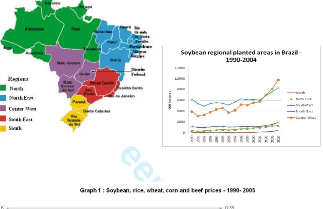
The soybean planted area in Brazil has known a tremendous growth from around 250 000 hectares in 1960 to 21,7 million hectares in 2009. Such expansion started in the South of the country, mainly in the States of Rio Grande do Sul and Parana during the 1960s, then continued through some states of the Centre-West (Minas Gerais, Goias and Mato Grosso do Sul) during the 1970s and the 1980s, and finally from 1990 until now, through the Northern of the Cerrado3 region (Mato Grosso particularly, Northern part of the State of Tocantins and Maranhão, Southern Part of the Para State), on the frontier with the Amazon basin (Bertrand and al. 2004 - see Figure 1.).

Insert Figure 1

In front of the rapid expansion through the Northern and Cerrado regions between 1990 and 2005, the first possible determinants that come to mind are exports, domestic output prices and the relative price of soybean with regards to other agricultural products. However, such prices have not clearly favoured soybean expansion ( see Graph 1), so other determinants have to be invoked, amongst which regional land prices, public research and exchange rates are possible good candidates (Bertrand and al. 2004).

Insert Graph 1

The Cerrado region, where most of the soybean expansion has occurred since 1990, has been colonized, firstly, by migrants mainly coming from the southern part of the country, then from closer states. The huge availability of land and low land prices are often cited, as farmers could sell a property of 150 -200 hectares in the South and acquire 800 to 1000 hectares in the States of the Cerrados region (Bertrand and al. 2004). Of course, in the meantime, this has led to an increase of land prices in the region, but the differential still persists (see graph 2). Low land prices in the Cerrado region is one of the reasons for Brazil’s soybean to be more competitive than that of the United States or Argentine, even with such competitiveness being partially offset by higher transport costs to maritime ports (Bertrand and al. 2004).

Insert Graph 2

Public research has also been an important vector of soybean expansion, since it has allowed the development of the culture in a region that was not adapted to former soybean varieties and agricultural technologies. Since the end of the 1970s, genetic research has allowed producing a variety adapted to the Cerrado regions, and several techniques have

3 _{For the graph exposed in the report, most of the Cerrado region pertains to the Center West macro region.}

3 4 5 6 7 8 9 10 11 12 13 14 15 16 17 18 19 20 21 22 23 24 25 26 27 28 29 30 31 32 33 34 35 36 37 38 39 40 41 42 43 44 45 46 47 48 49 50 51 52 53 54 55 56 57 58 59

For Peer Review

been developed to improve soils fertility. Such results led to yield improvements in all Brazilian States and particularly in the Cerrados region (see Graph 3).

Insert Graph 3

During the 2000s, 40 % to 60 % of the soybean production value came from exports to international markets. Thus, the exchange rate matters. Over the last years, the Brazil’s real currency’s low exchange rate has clearly favoured exportations. In 2004-2005 this trend was reversed as the US dollar dropped, leading to reduced international sales and accounting for, together with yields decrease, the observed diminution of planted areas after 2005. However, compared to other countries, the impact of exchange rate may be partially offset by the large size of Brazil’s domestic market.

In term of substitution/complementarities with other agricultural activities, one can expect substitution with beef, since a significant share of soybean plantations is established on former pasturelands. Cattle’s ranching in Brazil is mostly extensive and fed through pasture. For corn, the expected result is less clear because of the possibility in some regions of a harvest soybean / corn double harvest, with a small harvest of corn during the same year. In effect, around 75 % of the area planted is summer corn production while around 25 % of the area planted is winter corn production.

3. The model and methodology

3.1 The Economic Model

The desired acreage to be allocated to a crop i in period t ( d it

A ) is a function of expected relative prices in t ( e

it

p ), Zit the vector of risk variables and enabling factors (such as price risk, yield, factor price, climate variables...) in period t, and ε is the unobserved random _1it factor : it it e it d it p z A =α1+α2 +α3 +ε1 (1)

Because, a full adjustment of the desired allocation of land may not be possible in the short term, following Nerlove (1956), the change in acreage between periods is assumed to occur in proportion to the difference between desired acreage for the current period and observed acreage in the previous period :

it it d it it it A A A A = ₋₁+δ( − ₋₁)+ε₂ (2)

where Ait is the observed acreage planted of crop i, Ait−1 is the lagged observed planted

acreage of crop i, δis the partial-adjustment coefficient and ε_2ita random term with

it 2 ε

(

)

For Peer Review

The structural form equations (1) and (2) yield the reduced form:

it it e it t i it A p Z A =θ₀ +θ_{1 (−1)} +θ₂ +θ₃ +ν (3) with : 3 3 2 2 1 1 0 δα ;θ 1 δ;θ δα ,θ δα θ = = − = = it it it δε1 ε2 ν = +

The presence of the lagged dependent variable introduces autocorrelation in the error term. The previous model presents unobservable variables, the expected prices e

it

p . Observed prices are market or effective farms-gate price after production has occurred, while production decisions have to be based on the prices farmers expected to prevail several months later at harvest time. Modeling of expectation formation is thus necessary. Following Nerlove (1956), expectations are updated from one period to another in proportion of the difference between the observed and expected price levels of the previous period :

(

)

(

)

where 0< β <1 the adapted price coefficient:

Following Judge, Griffiths, Hill, Lutkepohl, & Lee, 1985, if the quasi-rational expectation

hypothesis is considered, then equation (4) can be expressed as an infinite-order AR(p)

process as follows (see also Kanwar (2006)):

(

)

∑

The estimation procedure requires specification of p. We pick the p = {1} by considering the parsimonious criterions and various stationary tests, such as the Schwarz criterion and the Ljung–Box–Pierce test. Substituting (5) in (3) yields the reduced form:

it it it t i it A p Z A =θ0 +θ1 (₋1) +θ2β1 ₋1 +θ3 +ν (6)

Such specification is similar with Kanwar (2006), Balcomb and Prakash (2000) and Barbosa (1986).

3.2. The data set

3 4 5 6 7 8 9 10 11 12 13 14 15 16 17 18 19 20 21 22 23 24 25 26 27 28 29 30 31 32 33 34 35 36 37 38 39 40 41 42 43 44 45 46 47 48 49 50 51 52 53 54 55 56 57 58 59

For Peer Review

The previous model has been used first to estimate the soybean supply response function in Brazil, first at the national level and then at the regional level, i.e. for the Centre-West region (new soybean production basin) and for the South-Southeast (older soybean production basin). The functions have been estimated for the period 1990-2004. Most of the data linked to the agricultural sector in Brazil are collected by IBGE, the Brazilian Statistics Institute. The data on soybean planted acreages, yield, production volumes and farmgate prices come from the Municipal Agricultural Production Survey (PAM), realized yearly since 1990 only. For beef price, cropland price, labor price, inflation rate, the data provided by the Getulio Vargas fundation have been used. They are usually mensal and nominal, available at the national and the states levels, so some computations have been made to get annual constant prices for each Brazilian state. Soybean export FOB values are provived by the Office of Foreign Trade which computes yearly export volume and export values for each Brazilian imported and/or exported commodity at the national and at the state levels. As was mentioned in introduction, Brazil is a large country and the soybean planted area is not spatially homogeneous i.e. there are a number of regional characteristics influencing supply, that vary from state to state yet are fixed in time. These features need to be

controlled in the regression model to avoid biasing the estimated coefficients. Moreover we had only 15 years of observations from 1990 to 2004. Panel data were thus used where the cross-section units are the soybean producing states (12 states). Such choice allows to control for spatial heterogeneity and produces more efficient estimated coefficients. At the national level, it thus gave us an initial sample of 180 observations. However, as soybean expansion is more recent in the Center-North of the country, some states of the region have registered soybean expansion only since 1996. (Tocantins, Piaui). The panel database was thus non-balanced and at the national level accounted for 124 observations. For regional estimation, the Centre-West region (Cerrados) is composed of 6 states (Tocantins, Piaui, Mato Grosso, Mato Grosso do Sul, Maranhão and Goias), and the South-Southeast region is composed of 5 states (Minas Gerais, São Paulo, Paraná, Santa Catarina and Rio Grande do Sul). This resulted in a sample of 64 observations for the Cerrados and 60 observations for the South-East region.

For each estimated model, the dependent variable is the soybean planted area. As Kanwar (2006), we chose to work with corn, soybean, and beef farm harvest prices and not with international FOB prices because for all of them part of the production is sold on the domestic market and the other on the international market. Moreover, it was not possible to separate winter and summer corn production prices, the farmgate price being an average annual price.

Following Kanwar (2006), Sadoulet and de Janvry (1995)), the other independent variables in the models are : soybean price variance (S2lnpsk,t), soybean yield and variance with a 3 4 5 6 7 8 9 10 11 12 13 14 15 16 17 18 19 20 21 22 23 24 25 26 27 28 29 30 31 32 33 34 35 36 37 38 39 40 41 42 43 44 45 46 47 48 49 50 51 52 53 54 55 56 57 58

For Peer Review

one year lag (Yieldk,t-1 , S2Yieldk,t-1), land price witha one year lag (P_landk,t-1) and the % of soybean production value sold on international markets (%Fobk,t)..

Variable definitions and sources are found in Appendix 1. Each variable means and standard deviations are reported in Appendix 2.

3.3. The Methodology

In order to estimate equation (6) for soybean, a Dynamic Panel Data has been pooled. Sending k, the state-level index, we have:

(6) kt k K k kt kt t k kt A p Z A =λ +λ +λ +λ

∑

The dependent variable Akt refers to acreage in Eq. (6) for state k. Variables Zkst denote the set of regressors chosen, µk is the unobservable individual-specific effect, νkt is the

remaining disturbance. With (0, 2)

µ σ µk ≈IID , and (0, ) 2 ν σ

νkt ≈IID . All variables – regressand and regressors – are in (natural) logs.

The problem with such Dynamic Panel Data regression is that it presents two sources of persistence over time (see, Baltagi (2005)): Autocorrelation due to the presence of lagged dependent variables among regressors and individual effects characterizing the heterogeneity among states. Since the Akt is a function of µk, it immediately follows that

Akt-1 is also a function of µk. Therefore Akt-1 is correlated with error term. This is enough to turn Ordinary Last Square (OLS) estimator biased and inconsistent even though νkt are not serially correlated. To solve this problem, one option could be to apply the fixed effect estimator (FE) that wipes out µk. However, Akt-1 and pkt-1 are correlated with νkt−1 by

construction, therefore as T is fixed, the FE estimator is biased and inconsistent4.

4 _{However, it is worth emphasizing that only if T→∝}

the FE is consistent for the dynamic error component model (see Nickell (1981)), unfortunately in our data base T is fixed and short.

3 4 5 6 7 8 9 10 11 12 13 14 15 16 17 18 19 20 21 22 23 24 25 26 27 28 29 30 31 32 33 34 35 36 37 38 39 40 41 42 43 44 45 46 47 48 49 50 51 52 53 54 55 56 57 58 59

For Peer Review

An alternative to wiping out the fixed effect is the first difference (FD) transformation. In this case, correlation between the predetermined explanatory variables and the remaining error is easier to handle (see, Baltagi (2005), cap. 8). The first differences get rid of the µk and, in practice, this allows to use past, present and future values of the strictly exogenous variables to build instruments for the lagged dependent variables and other non exogenous variables, once the permanent effect has been cancelled after differentiation (Anderson and Hsiao (1981)). Anderson and Hsiao (1981) suggest instrumental variable (IV) estimation method to estimate the first differentiated model. However, Arellano and Bond (1991) argue that this method leads to consistent but not necessarily efficient estimates of the parameter because it does not make use of all the available moment conditions. Therefore, they proposed a generalized method of moments (GMM) procedure that is more efficient than IV. In this paper, we have used the Arellano and Bond (1991) technique to estimate our dynamic panel model found in (7).

4. The Results

4.1. National level

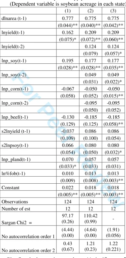
First of all, the complete data set has been used to estimate equation (7). The soybean acreage has been estimated as a function of nine sets of variables: the soybean area and price lagged, the yield lagged, two soybean substitute crops’ price lagged (corn and beef), and one input variable (land price). One control variable has been added (export share lagged) and two variables to take account for risk (price and yield variance). Following Berhman (1970), higher risk levels may decrease soybean acreage. All the explanatory variables are entered with one lag.

Table 1 report the results of three models. In column (1), equation (7) is estimated using one-step Arellano and Bond (1991) (AB) technique, assuming that all variables are strictly exogenous. In column (2), equation (7) is estimated using one-step AB technique, assuming that some variables are predetermined (soybean and corn prices lagged and yield lagged). The variable is said predetermined if E

[

]

[

]

lagged variables are used as instruments. Finally, in column (3), equation (7) is estimated assuming that soybean price and yield lagged are predetermined with the variance and covariance matrix robust to heteroskedasticity.

Interpreting table (1) column (1), the - Sargan test rejects the null hypothesis that the overidentifying restriction is valid to 5%. The null hypothesis of no first-order autocorrelation in residuals is rejected, but not the second-order no autocorrelation null hypothesis. First-order autocorrelation in residuals does not imply that estimates are inconsistent, just second-order autocorrelation.

3 4 5 6 7 8 9 10 11 12 13 14 15 16 17 18 19 20 21 22 23 24 25 26 27 28 29 30 31 32 33 34 35 36 37 38 39 40 41 42 43 44 45 46 47 48 49 50 51 52 53 54 55 56 57 58

For Peer Review

Estimating the model considering soybean and corn lagged prices and soybean lagged yield as predetermined variables (table 1, column 2) improves the results. The Sargan test cannot reject the null hypothesis that the over-identifying restriction is valid to 5% and the null hypothesis of no first-order and second-order autocorrelation in residuals can not be rejected. When the model presents a good specification, Arellano and Bond (1991) recommend using the one-step result for infering the coefficient because the two step stand errors tend to be biased downward in small sample.

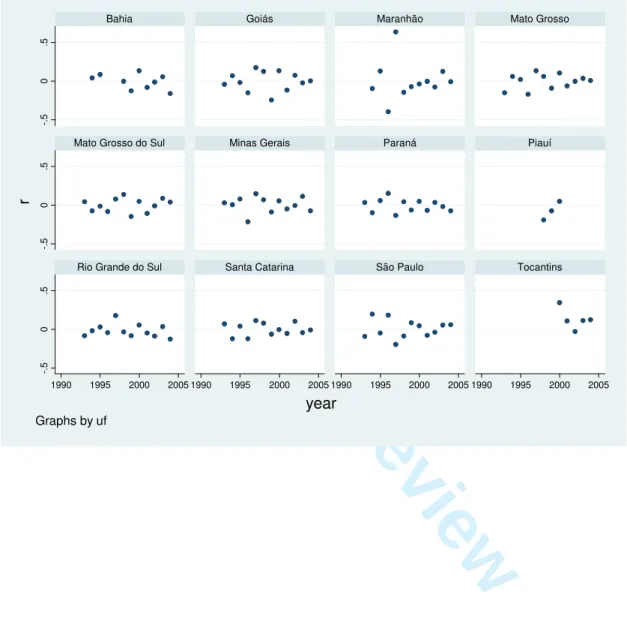
Appling the White matrix to heteroskedasticity correction (table 1, column 3) we cannot reject null hypothesis of no first-order and second-order autocorrelation at 5%. Comparing columns (2) and (3), standard errors are quit small in the column (3), suggesting heteroskedasticity. The residuals are plotted in the Appendix 3 (Figure A3a).

Analyzing the estimated coefficients in table 1 column (3), most coefficients are significant and have expected signs. The exportation share lagged coefficient is positive and significant but the coefficient is low. The yield lagged are significant and positive. Beef and corn first lagged coefficients are negative and significant at 5%, meaning that they are probably soybean substitutes at the national level. The beef price lagged coefficients are bigger than corn price lagged coefficients, suggesting that beef prices have stronger influence on soybean acreage than corn prices. The lagged price variance is significant at 10% and positive but the coefficient is not very high, suggesting that price variability does not impact strongly on supply. The soybean lagged yield variance is not significant. These two last results indicate that at the national level, soybean producers are not very risk averse. Finally, the lagged land price is not significant.

Insert Table 1.

Using the estimated coefficients in table 1 column 3, it is possible to calculate the own and cross price supply elasticity (see table 2). The short term own supply elasticity is the price lagged estimated coefficient, and the long term elasticity is calculated admitting that in the long term Pt

= Pt-1. In this case β in (8) is equal to one5.

In the long term, we can consider that soybean supply is price elastic (0.787). Beef is an important soybean substitute with cross price elasticity (-0.822). On the other hand, analyzing the cross price elasticity with corn, it appears to be substitute and inelastic (-0.222).

Insert table 2.

4.2. Regional Level

5 _{For more details, see Sadoulet and de Janvry (1995, cap 4)}

3 4 5 6 7 8 9 10 11 12 13 14 15 16 17 18 19 20 21 22 23 24 25 26 27 28 29 30 31 32 33 34 35 36 37 38 39 40 41 42 43 44 45 46 47 48 49 50 51 52 53 54 55 56 57 58 59

For Peer Review

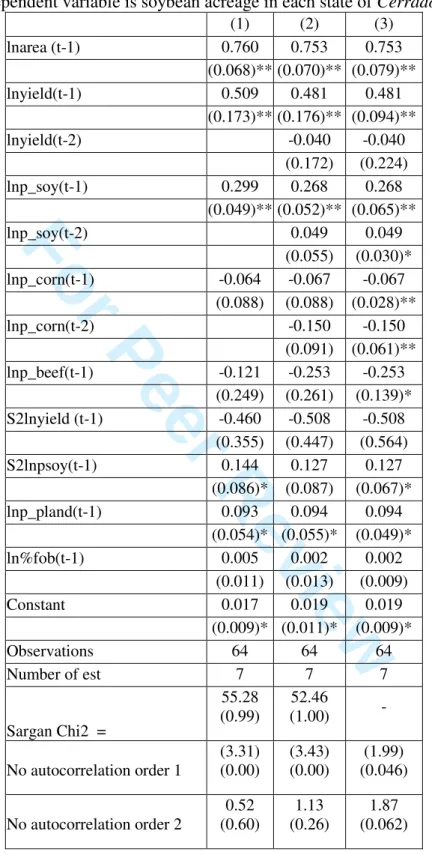
The aim is now to estimate separately soybean supply elasticity for the Cerrados and

South-South East regions. The hypothesis is that own and cross price elasticity may

strongly differ between these two regions.

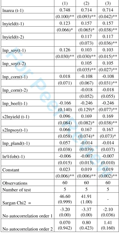
Tables 3 and 4 display the results of soybean supply estimation for Cerrado and South-

Southeast respectively. In both cases, the one-step GMM AB technique is used. As in table

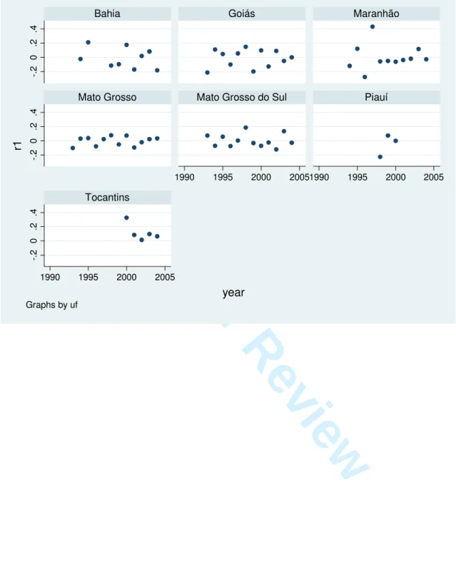
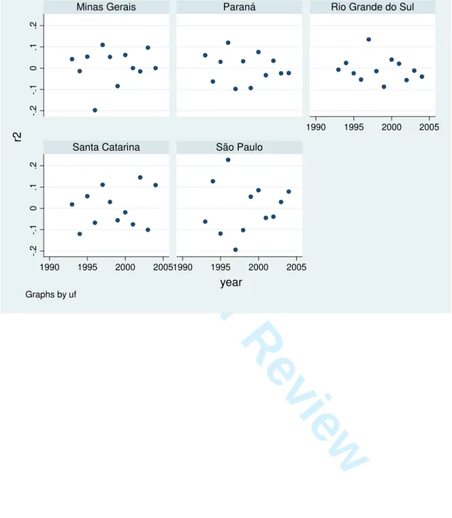
1, equation (7) is first estimated assuming that all variables are strictly exogenous (first column). In the second column, soybean lagged price and yield are predetermined and the model is estimated using GMM with IV. Finally, in column 3, the GMM with IV is again estimated, but with coefficients robust to heteroskedasticity. Residuals are plotted in the Appendix 3 (Figure A3b and A3c).

Analyzing the identification conditions in tables 3 and 4, the over-identification null hypothesis is rejected even in column (1), possibly because the Sargan test is not powerful enough with small data. In both models, the null hypothesis of no second order autocorrelation cannot be rejected. As in the previous section, only the results found in column (3) are analyzed because the coefficients are robust to heteroskedasticity.

Comparing Regions 1 and 2 (tables 3 and 4), soybean lagged planted acreage and price coefficients are significant and have expected signs. In both regions, beef and corn price coefficients are different from zero. As for the input coefficient, land price lagged is significant only in Cerrado at 10%, but with a positive (and non expected) sign, maybe because of land speculation. In any case, it indicates that land price can still increase in the region without having a negative impact on supply. Exportation share is not significant in both regions.

Insert Table 3

For risk variables, only price variability appears to be significant in the Cerrados and with a positive sign, suggesting again that soybean price variability did not have a negative impact on supply and that producers are rather risk takers. The same occurs in the South-Southeast where yield variance is also significant and with a positive sign. It must be underlined that yields have systematically increased over the 1990-2004 period with very short periods of yields decrease. Soybean producers are probably quite confident on this respect.

Insert Table 4

The regions 1 and 2 long and short term own and cross price elasticity are found in table 5. For own price elasticity, a clear difference appears between both regions: the long term soybean supply is very price elastic in the Center-West region (1.085) and its own price elasticity is much higher than in the South-Southeast region (0.360).

In both regions beef appears as a soybean substitute. The substitution is easier in the

Cerrado (-1,024) than in the South (-0.860). Corn is a soybean substitute crop in South

(-0.378) and in Cerrados (-0.271). 3 4 5 6 7 8 9 10 11 12 13 14 15 16 17 18 19 20 21 22 23 24 25 26 27 28 29 30 31 32 33 34 35 36 37 38 39 40 41 42 43 44 45 46 47 48 49 50 51 52 53 54 55 56 57 58

For Peer Review

The computed elasticity presented at the national and regional levels allow to assess the variation of soybean planted area in function of soybean, beef and corn prices variations. At the national level, the results suggest that a 1% increase of soybean price could translate into a 17% and 79 % increase of the soybean planted area respectively in the short term and the long term. The results at the regional levels suggest that such increase may occur mainly in the Cerrado region. Looking at cross price elasticity, the results suggest that a 1 % increase of beef price may translate into a 18% and 88 % reduction of the soybean planted areas respectively in the short and long term, suggesting a high substitution between beef and soybean, particularly in the Cerrado region. Substitution between corn and soybean also exist but with much lower elasticity at the national and regional levels. One limit of the methodology is that it does not allow to assess precisely the possible variation of soybean planted areas when several prices are simultaneously increasing or decreasing a lot, at it occurred during the price spike of 2007-2008.

5. Conclusion

The estimation of soybean supply in Brazil underlines that the commodity has been price elastic over the 1990-2004 period and that any price increase may thus translate into high production growth rate, unless new limiting factors appear. At the national level, corn and beef appear both as soybean substitutes.

Refining the estimation to differentiate older production basins (South – South East) from the new soybean expansion frontier (Cerrados) shows that the agrichain’s possible response to improving international markets access may be quite distinct. The own price elasticity in Cerrados is more than three times higher than in the South-South East. It is clear that any international price increase is likely to speed up the expansion of soybean in the Cerrados, as occurred over the last 15 years, unless new determinants appears to restrain this movement. The minimum (South-South east) and maximum (Cerrados) elasticity levels found shall be used to realize sensitivity analysis of world agricultural trade models results used to simulate trade liberalization scenarios. Current Brazil soybean supply elasticity found in FAPRI for example is quite low (0,34) and may underestimate Brazil supply response to increasing international prices in the long term

(http://www.fapri.org/tools/elasticity.aspx).

Whereas it was believed that land prices could be an important determinant of soybean supply, this does not appear significant in the different regressions. This factor should not be construed as negligible, as it has been shown that low land price in Cerrados

3 4 5 6 7 8 9 10 11 12 13 14 15 16 17 18 19 20 21 22 23 24 25 26 27 28 29 30 31 32 33 34 35 36 37 38 39 40 41 42 43 44 45 46 47 48 49 50 51 52 53 54 55 56 57 58 59

For Peer Review

explains a large part of the Brazilian soybean competitiveness. However, it may increase in this region without necessarily having a negative impact on supply growth.

Finally, an important debate exists in Brazil on whether soybean is responsible for putting more pressure on the Amazon forest or if it allows land use intensification through the restoration of degraded pasturelands (Brandão and al. 2005). As shown in Figure 1, soybean expansion has occurred along the border of the Amazon region. Recently, based on satellite image analysis of the State of Mato Grosso, Morton and al. (2006) estimated that direct forest conversion for crop production amounts to a maximum of 25% of the total deforested area. Our results confirm high substitution between beef and soybean along the Amazon border. The pressure of the sector on the Amazon forest has been mainly indirect through the probable displacement of cattle ranching to the Amazon region. Specific private or public regulations should be implemented to reinforce land use intensification through pasture-soybean-corn rotation.

6. Cited references

ANDERSON, T. W.; HSIAO, C. (1981). Formulation and Estimation of Dynamic Models Using Panel Data. Journal of Econometrics 18, 570-606.

ARELLANO, M.; BOND, S. (1991). Some Tests of Specification for Panel Data: A Monte Carlo Evidence and an Application to Employment Equations. The Review of Economic

Studies 58(2 – 194), 277-297.

BALCOMB, K., PRAKASH A. (2000). Estimating the long run supply and demand for agriculture labor in UK. European Review of Agricultural Economics 27(2), 157-66 BALTAGI, B. (2005). Econometric Analyses of Panel Data. IE-WILEY, England 3rd Edition

BARBOSA, M. M. T. L. (1986) Análise da oferta de soja sob a abordagem de expectativas racionais. Máster Degree – Federal University of Viscosa (Brazil).

BEHRMAN, J.R. (1970). Supply Response in Underdeveloped Agriculture: A Case Study of Four Major Annual Crops in Thailand, 1937-1963. Journal of Economic Literature 8(2), 459-462.

BERTRAND J.P., PASQUIS R., DE MELLO N.A., and al. (2004). L’analyse des

déterminants de l’avancée du front soja en Amazonie Brésilienne : le cas du Mato Grosso.

Rapport INRA-CIRAD, Paris : CIRAD.

3 4 5 6 7 8 9 10 11 12 13 14 15 16 17 18 19 20 21 22 23 24 25 26 27 28 29 30 31 32 33 34 35 36 37 38 39 40 41 42 43 44 45 46 47 48 49 50 51 52 53 54 55 56 57 58

For Peer Review

BRANDÃO, A; REZENDE,G; MARQUES, R (2005). Crescimento Agrícola no Brasil no

Período 1999-2004: Explosão da Soja e da Pecuária Bovina e seu Impacto sobre o Meio

Ambiente. IPEA, Texto para Discussão n. 1103, Rio de Janeiro: IPEA.

JUDGE, G. G., W. E. GRIFFITHS, R. C. HILL, H. LUTKEPOHL, and T.C. LEE (1985).

The Theory and Practice of Econometrics, (2nd ed.), New York: John Wiley & Sons.

KANWAR; S. (2006) Relative profitability, supply shifters and dynamic output response, in a developing economy. Journal of Policy Modelling 28, 67–88

MAMINGI N. (1996). How Prices and Macroeconomic Policies Affect Agricultural Supply

and the Environment Washington DC: The World Bank Policy Research Department

Environment, Infrastructure, and Agriculture Division

MORTON D.C., DE FRIES R.S., SHIMABUKURO Y.E., ANDERSEN L.O., ARAI E., BON ESPITITO SANTO F., FREITAS R., MORISETTE J. (2006). Cropland expansion changes deforestation dynamics in the southern Brazilian Amazon. PNAS, 103 (39), 14637-14641

NERLOVE, M. (1956). Estimates of Supply of Selected Agricultural Commodities.

Journal of Farm Economics 38, 496-509.

NICKELL, S. (1981). Biases in dynamic models with fixed effects. Econometrica, 49 (6), 417-426.

OECD (Organisation for Economic Co-operation and Development) (2006).

Documentation of the AGLINK Model. Working Party on Agricultural Policies and Markets, AGR-CA-APM(2006)16/FINAL. Directorate for Food, Agriculture and Fisheries,

Committee for Agriculture, OECD, Paris.

SADOULET, E.; JANVRY A. (1995) Quantitative Development Policy Analysis. Baltimore, London: The Johns Hopkins University Press.

THERY H., DE MELLO N.A., (2005). Diversités et mobilité de l’agriculture brésilienne.

Cahiers Agricultures 14 (1), 11-18. 3 4 5 6 7 8 9 10 11 12 13 14 15 16 17 18 19 20 21 22 23 24 25 26 27 28 29 30 31 32 33 34 35 36 37 38 39 40 41 42 43 44 45 46 47 48 49 50 51 52 53 54 55 56 57 58 59

For Peer Review

Appendix 1 Indices and Variables definition and sources Indices :

k : Brazilian states considered {Tocantins, Maranhão, Piauí, Bahia, Minas Gerais, São Paulo, Parana, Santa Catarina, Rio Grande do Sul, Mato Grosso, Mato Grosso do Sul, Goiás}

t : time {1990-2004}

Variables definition and sources

Acreagek,t : Soybean planted area in state k at time t (hectare). Source : www.ibge.com.br Yieldk,t : Soybean yield in state k at time t (kg/hectare). Source : www.ibge.com.br S2lnpsoyk,t: Soybean producer price variance in state k at time t. Sources :

www.ibge.com.br and www.fgvdados.com.br

S2lnpyieldk,t: Soybean yield variance in state k at time t. Sources : www.ibge.com.br P_soyk,t: Soybean constant producer price at time t in state k ($Reais of 2004/kg). Source:

www.ibge.com.br and www.fgvdados.com.br

P_beefk,t: Beef constant producer price at time t in state k ($Reais of 2004 / 15kg). Source

: www.fgvdados.com.br

P_cornk,t : Corn constant producer price at time t in state k ($Reais of 2004 / kg). Source :

www.ibge.com.br and www.fgvdados.com.br

P_landk,t: Cropland selling price at time t in state k ($Reais of 2004/hectare). Source:

www.fgvdados.com.br

% Fobk,t : Soybean export value / Soybean production value *100 (%). Sources : www.aliceweb.desenvolvimento.gov.br and www.ibge.com.br

3 4 5 6 7 8 9 10 11 12 13 14 15 16 17 18 19 20 21 22 23 24 25 26 27 28 29 30 31 32 33 34 35 36 37 38 39 40 41 42 43 44 45 46 47 48 49 50 51 52 53 54 55 56 57 58

For Peer Review

Appendix 2. Means and Standard Deviations of each variable (all the variable are in natural log)

Observations Mean Std Dev. Min Max

Acreage 180 12.98 1.80 7.35 15.48 Yield 180 7.64 0.32 5.61 8.03 P_Soy 168 -0.42 0.40 -1.29 1.09 P_Beef 156 4.11 0.12 3.81 4.39 P_Corn 168 -0.99 0.30 -1.75 -0.15 P_Land 175 7.57 1.05 4.76 9.35 % Fob 165 3.20 1.27 -5.79 5.28 S2lnpsoy 156 0.17 0.25 0.00 1.82 S2lnpyield 156 0.11 0.37 0.00 3.44

Source: Elaborated by the authors.

3 4 5 6 7 8 9 10 11 12 13 14 15 16 17 18 19 20 21 22 23 24 25 26 27 28 29 30 31 32 33 34 35 36 37 38 39 40 41 42 43 44 45 46 47 48 49 50 51 52 53 54 55 56 57 58 59

For Peer Review

Table A3a: Residuals of the estimation of table 1 column 3.

-. 5 0 .5 -. 5 0 .5 -. 5 0 .5 1990 1995 2000 2005 1990 1995 2000 2005 1990 1995 2000 2005 1990 1995 2000 2005

Bahia Goiás Maranhão Mato Grosso

Mato Grosso do Sul Minas Gerais Paraná Piauí

Rio Grande do Sul Santa Catarina São Paulo Tocantins

r year Graphs by uf 3 4 5 6 7 8 9 10 11 12 13 14 15 16 17 18 19 20 21 22 23 24 25 26 27 28 29 30 31 32 33 34 35 36 37 38 39 40 41 42 43 44 45 46 47 48 49 50 51 52 53 54 55 56 57 58

For Peer Review

Table A3b: Residuals from estimated model in table 3 column 3 (Cerrado).

-. 2 0 .2 .4 -. 2 0 .2 .4 -. 2 0 .2 .4 1990 1995 2000 20051990 1995 2000 2005 1990 1995 2000 2005

Bahia Goiás Maranhão

Mato Grosso Mato Grosso do Sul Piauí

Tocantins r1 year Graphs by uf 3 4 5 6 7 8 9 10 11 12 13 14 15 16 17 18 19 20 21 22 23 24 25 26 27 28 29 30 31 32 33 34 35 36 37 38 39 40 41 42 43 44 45 46 47 48 49 50 51 52 53 54 55 56 57 58 59

For Peer Review

Table A3c: Residuals from estimated model in table 3 column 3 (South-Southeast).

-. 2 -. 1 0 .1 .2 -. 2 -. 1 0 .1 .2 1990 1995 2000 2005 1990 1995 2000 20051990 1995 2000 2005

Minas Gerais Paraná Rio Grande do Sul

Santa Catarina São Paulo

r2 year Graphs by uf 3 4 5 6 7 8 9 10 11 12 13 14 15 16 17 18 19 20 21 22 23 24 25 26 27 28 29 30 31 32 33 34 35 36 37 38 39 40 41 42 43 44 45 46 47 48 49 50 51 52 53 54 55 56 57 58

For Peer Review

Crop/Region Price/Data type

Authors Method Price Variable S.R.EL L.R.E L Lags Coffee Kenya (industry) 1946-64 (Time S.) Maitha (1970) Nelove type Pr 0.15* 0.38* Pr,t-1_t-1 Cotton Uganda-Buganda 1922-38 (Time S.) Frederick (1969) OLS Pcof 0.25-0.67* 0.25-0.67* Pcof,,t-1 Ghana 1968-81 (Time S.) Seini (1985) Nerlove Pn 0.55* 1.32* Pn, t-1 Wheat Kenya (Nyandurua) 1965-83 (Time S.)

Kere et. al. Nerlove Pn 0.65* 1.38 Pn, t-1

Cocoa Western Nigeria 1970 (Cross S.) Olayemy and Oni (1972) OLS Piin Pdin 1.217* 0.643* 0.25 0.67* Piin, t Pdin, t Onion USA 1952- 74 (Time S.) 1952- 74 (Time S.) 1952- 74 (Time S.)

Trail et. al. (1978) Trail et. al. (1978) Trail et. al. (1978) OLS OLS OLS Pip PiiW PdW PmmW PdmmW 0.105* 0.09* 0.068* 0.442* 0.086* Pip, t-1 PiiW, t-1 PdW, t-1 PmmW, t-1 PdmmW, t-1 Paddy Sri Lanka 52-87

(Time S.) Gunawardana & Ockzowski (1992) OLS Pf 0.05* 0.06* Pf, t-1 Sugar Cane Bangladesh 1951-81 (Time S.) 1951-81 (Time S.) Jaforulah (1993) Jaforulah (1993) NLS NLS Pip PimW PdmW 0.30* 0.32* 0.15 0.45* 0.41* 0.20* Pip, t PimW, t PdmW, t Crop Area 58 DCs and LDCs Panel Binswanger et.al. (1987) Within Pi 0,011* Pi, t Source: Mamingi (1996).

Notes: Time S.: time series. Cross S. cross section. Price variable: type of real output price variable. Pris the

ratio of nominal price of coffee to the import price índex. Pcof is the ratio of cotton price of coffee price. Pn is 3 4 5 6 7 8 9 10 11 12 13 14 15 16 17 18 19 20 21 22 23 24 25 26 27 28 29 30 31 32 33 34 35 36 37 38 39 40 41 42 43 44 45 46 47 48 49 50 51 52 53 54 55 56 57 58 59

For Peer Review

nominal price of cotton which is used separately with the price of groundnut. Pi in and P

d

in are raising and

falling prices, respectively, from direct interviews (see above under Olayemi and Oni). Pip is the regular real

price. Pi

W and PdW are rising and falling prices à la Wolfram6. PimW and PdmW are rising and falling prices,

respectively using modified Wolfram technique7. Pf is the ratio of guaranteed price parity (PPP) exchange rate

deflated to 1980 prices using the ptrice index for the OCDE as whole. S.R.El.: short-run price elasticity. L.R.El.: long run price elasticity. Lags: lags used price. *significant at the 10% level, at least.

6

See equations (7) and (8) in: Mamingi, Nlandu “How Prices and M acroeconomic Policies Affect Agricultural Supply and the Environment” The World Bank Policy Research Department Environment, Infrastructure, and Agriculture Division September 1996.

7

See equations (9) and (10) in: Mamingi, Nlandu “How Prices and M acroeconomic Policies Affect Agricultural Supply and the Environment” The World Bank Policy Research Department Environment, Infrastructure, and Agriculture Division September 1996.

3 4 5 6 7 8 9 10 11 12 13 14 15 16 17 18 19 20 21 22 23 24 25 26 27 28 29 30 31 32 33 34 35 36 37 38 39 40 41 42 43 44 45 46 47 48 49 50 51 52 53 54 55 56 57 58

For Peer Review

Figure 1: Soybean regional expansion in Brazil 1990-2004 (source IBGE) 3 4 5 6 7 8 9 10 11 12 13 14 15 16 17 18 19 20 21 22 23 24 25 26 27 28 29 30 31 32 33 34 35 36 37 38 39 40 41 42 43 44 45 46 47 48 49 50 51 52 53 54 55 56 57 58 59

For Peer Review

Graph 2 : Land prices (pasture) 1990 and 2004 ($Reais 2004)

0 1000 2000 3000 4000 5000 6000 1990 2004 R e a is /h a Brasil Para Mato Grosso Tocantins Rio Grande do Sul Parana

Source : fgvdados.com.br

Graph 3 : Soybean Yield in Brazil 1990-2005

0 500 1000 1500 2000 2500 3000 3500 1990 1991 1992 1993 1994 1995 1996 1997 1998 1999 2000 2001 2002 2003 2004 2005

Source : IBGE, PAM

k g /h e c ta re Norte Nordeste Sudeste Sul Centro-Oeste Source : www.ibge.com.br 3 4 5 6 7 8 9 10 11 12 13 14 15 16 17 18 19 20 21 22 23 24 25 26 27 28 29 30 31 32 33 34 35 36 37 38 39 40 41 42 43 44 45 46 47 48 49 50 51 52 53 54 55 56 57 58

For Peer Review

Table 1: Soybean Supply estimation

(Dependent variable is soybean acreage in each state)

(1) (2) (3) dlnarea (t-1) 0.777 0.775 0.775 (0.044)** (0.040)** (0.042)** lnyield(t-1) 0.162 0.209 0.209 (0.075)* (0.072)** (0.060)** lnyield(t-2) 0.124 0.124 (0.079) (0.057)* lnp_soy(t-1) 0.195 0.177 0.177 (0.028)** (0.028)** (0.035)** lnp_soy(t-2) 0.049 0.049 (0.031) (0.022)* lnp_corn(t-1) -0.067 -0.050 -0.050 (0.058) (0.052) (0.015)** lnp_corn(t-2) -0.095 -0.095 (0.050) (0.052) lnp_beef(t-1) -0.130 -0.185 -0.185 (0.129) (0.125) (0.058)** s2lnyield (t-1) -0.037 0.086 0.086 (0.109) (0.100) (0.054) s2lnpsoy(t-1) 0.066 0.080 0.080 (0.054) (0.050) (0.032)* lnp_pland(t-1) 0.070 0.057 0.057 (0.033)* (0.033) (0.031) ln%fob(t-1) 0.010 0.013 0.013 (0.009) (0.008) (0.003)** Constant 0.022 0.018 0.018 (0.005)** (0.005)** (0.003)** Observations 124 124 124 Number of est 12 12 12 Sargan Chi2 = 97.17 (0.26) 110.42 (0.99) - No autocorrelation order 1 (4.44) (0.00) (4.64) (0.00) (1.91) (0.056) No autocorrelation order 2 0.43 (0.67) 1.21 (0.23) 1.22 (0.221) Obs: Standard errors in parentheses ** significant at 5%; * significant at 10%. The column (3) is robust to heterocedasticity. 3 4 5 6 7 8 9 10 11 12 13 14 15 16 17 18 19 20 21 22 23 24 25 26 27 28 29 30 31 32 33 34 35 36 37 38 39 40 41 42 43 44 45 46 47 48 49 50 51 52 53 54 55 56 57 58 59

For Peer Review

price supply elasticities. National level Brasil LT ST soybean 0.787 0.177 corn -0.222 -0.050 beef -0.822 -0.185 3 4 5 6 7 8 9 10 11 12 13 14 15 16 17 18 19 20 21 22 23 24 25 26 27 28 29 30 31 32 33 34 35 36 37 38 39 40 41 42 43 44 45 46 47 48 49 50 51 52 53 54 55 56 57 58

For Peer Review

Table 3: Soybean Supply estimation in Brazilian Cerrado (Dependent variable is soybean acreage in each state of Cerrado)

(1) (2) (3) lnarea (t-1) 0.760 0.753 0.753 (0.068)** (0.070)** (0.079)** lnyield(t-1) 0.509 0.481 0.481 (0.173)** (0.176)** (0.094)** lnyield(t-2) -0.040 -0.040 (0.172) (0.224) lnp_soy(t-1) 0.299 0.268 0.268 (0.049)** (0.052)** (0.065)** lnp_soy(t-2) 0.049 0.049 (0.055) (0.030)* lnp_corn(t-1) -0.064 -0.067 -0.067 (0.088) (0.088) (0.028)** lnp_corn(t-2) -0.150 -0.150 (0.091) (0.061)** lnp_beef(t-1) -0.121 -0.253 -0.253 (0.249) (0.261) (0.139)* S2lnyield (t-1) -0.460 -0.508 -0.508 (0.355) (0.447) (0.564) S2lnpsoy(t-1) 0.144 0.127 0.127 (0.086)* (0.087) (0.067)* lnp_pland(t-1) 0.093 0.094 0.094 (0.054)* (0.055)* (0.049)* ln%fob(t-1) 0.005 0.002 0.002 (0.011) (0.013) (0.009) Constant 0.017 0.019 0.019 (0.009)* (0.011)* (0.009)* Observations 64 64 64 Number of est 7 7 7 Sargan Chi2 = 55.28 (0.99) 52.46 (1.00) - No autocorrelation order 1 (3.31) (0.00) (3.43) (0.00) (1.99) (0.046) No autocorrelation order 2 0.52 (0.60) 1.13 (0.26) 1.87 (0.062)

Obs: Standard errors in parentheses ** significant at 5%; * significant at 10%. The column (3) is robust to heterocedasticity 3 4 5 6 7 8 9 10 11 12 13 14 15 16 17 18 19 20 21 22 23 24 25 26 27 28 29 30 31 32 33 34 35 36 37 38 39 40 41 42 43 44 45 46 47 48 49 50 51 52 53 54 55 56 57 58 59

For Peer Review

Table 4: Soybean Supply estimation in Southern Brazil (Dependent variable is planted acreage)

(1) (2) (3) lnarea (t-1) 0.748 0.714 0.714 (0.100)** (0.093)** (0.042)** lnyield(t-1) 0.123 0.157 0.157 (0.066)* (0.065)* (0.038)** lnyield(t-2) 0.117 0.117 (0.073) (0.036)** lnp_soy(t-1) 0.126 0.103 0.103 (0.030)** (0.030)** (0.015)** lnp_soy(t-2) 0.105 0.105 (0.035)** (0.027)** lnp_corn(t-1) 0.018 -0.108 -0.108 (0.071) (0.067) (0.031)** lnp_corn(t-2) -0.018 -0.018 (0.052) (0.055) lnp_beef(t-1) -0.166 -0.246 -0.246 (0.140) (0.129)* (0.077)** s2lnyield (t-1) 0.096 0.169 0.169 (0.084) (0.082)* (0.038)** s2lnpsoy(t-1) 0.066 0.167 0.167 (0.058) (0.074)* (0.073)* lnp_pland(t-1) 0.057 -0.014 -0.014 (0.038) (0.039) (0.037) ln%fob(t-1) -0.006 -0.007 -0.007 (0.015) (0.013) (0.010) Constant 0.023 0.019 0.019 (0.006)** (0.006)** (0.002)** Observations 60 60 60 Number of test 5 5 5 Sargan Chi2 = 46.60 (0.999) 41.91 (1.00) - No autocorrelation order 1 -3.20 (0.00) -3.37 (0.00) -2.10 (0.036) No autocorrelation order 2 0.070 (0.942) 0.80 (0.423) 1.41 (0.160) 3 4 5 6 7 8 9 10 11 12 13 14 15 16 17 18 19 20 21 22 23 24 25 26 27 28 29 30 31 32 33 34 35 36 37 38 39 40 41 42 43 44 45 46 47 48 49 50 51 52 53 54 55 56 57 58

For Peer Review

Obs: Standard errors in parentheses ** significant at 5%; * significant at 10%. The column (3) is robust to heterocedasticity.

Table 5: Own price and cross price supply elasticities in Regions I (Center-West - Cerrado)

and II (South-South_East). I II LT ST LT ST soybean 1.085 0.268 0.360 0.103 Corn -0.271 -0.067 -0.378 -0.108 Beef -1.024 -0.253 -0.860 -0.246 3 4 5 6 7 8 9 10 11 12 13 14 15 16 17 18 19 20 21 22 23 24 25 26 27 28 29 30 31 32 33 34 35 36 37 38 39 40 41 42 43 44 45 46 47 48 49 50 51 52 53 54 55 56 57 58 59