Publisher’s version / Version de l'éditeur:
Vous avez des questions? Nous pouvons vous aider. Pour communiquer directement avec un auteur, consultez la première page de la revue dans laquelle son article a été publié afin de trouver ses coordonnées. Si vous n’arrivez pas à les repérer, communiquez avec nous à [email protected].
Questions? Contact the NRC Publications Archive team at
[email protected]. If you wish to email the authors directly, please see the first page of the publication for their contact information.
https://publications-cnrc.canada.ca/fra/droits
L’accès à ce site Web et l’utilisation de son contenu sont assujettis aux conditions présentées dans le site LISEZ CES CONDITIONS ATTENTIVEMENT AVANT D’UTILISER CE SITE WEB.
Laboratory Technical Report (National Research Council of Canada. Aerospace. Aerodynamics Laboratory); no. LR-AL-2020-0079, 2020-05-05
READ THESE TERMS AND CONDITIONS CAREFULLY BEFORE USING THIS WEBSITE.
https://nrc-publications.canada.ca/eng/copyright
NRC Publications Archive Record / Notice des Archives des publications du CNRC :
https://nrc-publications.canada.ca/eng/view/object/?id=9147610b-dbe9-443b-b77a-cbb15eb3a28e https://publications-cnrc.canada.ca/fra/voir/objet/?id=9147610b-dbe9-443b-b77a-cbb15eb3a28e
Archives des publications du CNRC
For the publisher’s version, please access the DOI link below./ Pour consulter la version de l’éditeur, utilisez le lien DOI ci-dessous.
https://doi.org/10.4224/40002057
Access and use of this website and the material on it are subject to the Terms and Conditions set forth at
Analysis of fast-response Cobra probe data in highly turbulent wake
flows
Analysis of Fast-Response Cobra Probe Data in Highly Turbulent Wake
Flows
Alanna Wall, Richard Lee, Hali Barber
1. Abstract
A fast-response Cobra probe is a specialized flow measurement instrument, developed by Turbulent Flow Instrumentation of Australia as described in Hooper and Musgrove (1997). This instrument is extremely useful for the study of bluff body wakes because it senses three-components of flow speed at high fre-quency with a small measurement head. It is inex-pensive and easy to use and is therefore an excellent choice for flow measurement projects where time and budget are major considerations. However, Cobra probes have a limitation on flow angle measurement that can lead to incomplete data sets for highly turbu-lent flows. Using a recent ship-airwake experiment as an example, this paper shows how probability dis-tributions of turbulence can be used to increase the usefulness of Cobra data in highly turbulent flows by providing additional insight into the flow characteris-tics that are affected by the limitation. The concepts shown in this paper are useful both for the analysis of flow characteristics and for validation of computa-tional fluid dynamics (CFD).
2. Introduction
A fast-response Cobra probe (Series 100), shown in Figure 1, is a specialized flow measurement instru-ment, developed by Turbulent Flow Instrumentation of Australia as described in Hooper and Musgrove (1997)). Cobra probes are fast-response pressure in-struments, measuring three-components of flow ve-locity and static pressure. Cobra probes are ideal for the study of turbulent flow because of their frequency response, and also because their heads are 2.5 mm
Email address: [email protected] (Alanna Wall)
wide which affords the measurement of small flow structures with minimal interference. It is inexpensive and easy to use and is therefore an excellent choice for flow measurement projects where time and budget are major considerations. The advantages of Cobra probes are discussed at length by Mallipudi and Selig (2004). The Bluff Body Aerodynamics Group at the National Research Council (NRC) owns several Co-bra probes and routinely uses them for the study of complex flows in the wakes of bluff bodies because of their many advantages.
Cobra probes have a limitation that affects the study of highly turbulent flows: their angular range. The probes only measure flow angles within ±45◦ of the longitudinal axis of the probe tip. This means that for highly turbulent or recirculating flow asso-ciated with the near wakes of bluff bodies, it can be impossible to measure a complete time-series at high sampling rates. The instruments are capable of mea-suring frequency components up to 1500 Hz. Instan-taneous flow measurements that fall outside of this “acceptance cone” of ±45◦register as zero in the re-sulting measurement time-series. This effect is known as “clipping”. Since the probes are practical for the measurement of bluff body flows, due to their ease of use, fast-response, and size, the NRC has devel-oped methods for using clipped-flow measurements reliably in the study of bluff body aerodynamics. This paper discusses those methods.
As part of a body of work spanning decades which supports helicopter operations for the Royal Canadian Navy (RCN) and Royal Canadian Air Force (RCAF), NRC routinely characterizes ship airwake flows us-ing wind tunnel experiments on subscale ship models. NRC is part of the North Atlantic Treaty Organiza-tion (NATO) Applied Vehicle Technologies (AVT) working groups focussed on international
collabora-tions on simulation support for shipboard-helicopter operations. The most recent working group, AVT-315: Comparative Assessment of Modeling and Sim-ulation Methods of Shipboard Launch and Recovery of Helicoptersdescribed in AVT-315 Research Task Group (2017), is using standardized conditions to benchmark national methods and improve standard-ization. The standardized ship geometry, known as the Generic Destroyer (GD), is described in public literature by Owen et al. (2021) and is available for public download at Wall et al. (2021).
Part of the NRC’s contribution to the NATO work-ing group involves the measurement of the airwake over the flight deck of a 1:50 scale model of the GD us-ing Cobra probes; the experimental setup is shown in Figure 2. Airwake data collected experimentally are intended, among other purposes, for the validation of CFD results generated by collaborating nations. The airwake data is available for public download at Wall et al. (2021). The Cobra probe clipped-airwake data present certain challenges associated with performing validation, which can be overcome, as demonstrated in this paper.
The NRC selected the Cobra probes for this test, knowing their limitations, because of their efficiency and reliability. The NRC has significant expertise in the area of interpreting highly turbulent flows, and this expertise is used in the interpretation of the data in this test despite the clipping phenomenon. Co-bra probes are widely used in open literature for the study of turbulent flows as given by Hanfeng et al. (2016), White et al. (2012), and Bell et al. (2016); however, these studies all collected unclipped data. In some cases, the avoidance of clipping can be achieved by tuning the orientation of the probe head for each data point; this strategy is effective for some turbulent flows but not for all. The authors were unable to find any studies interpreting clipped Cobra data, which is the focus of this current paper.
3. Methodology 3.1. Cobra Probes
The Series 100 Cobra probe used by NRC is a fast-response, four-hole pressure probe that provides dynamic, three-component velocity and static pres-sure meapres-surements up to a maximum speed of 107 kts
(55 m/s) within an acceptance cone of ±45◦. The probe features a multi-faceted head containing four pressure taps, each connected to a pressure transducer located nearby in the body in the probe. The close proximity of the pressure transducers, in combination with the short tubing, allows for correction of the fre-quency response of the system with a resolution up to 1.5 kHz, above which built-in electronics filter the output voltage signals as described by Hooper and Musgrove (1997).
In a typical setup, such as the one used for the NATO test, the static-pressure port of the probe is connected to the wind tunnel barometric pressure ref-erence located in the wind tunnel contraction. The four ports of the Cobra probe are connected to a stan-dard data acquisition system that acquires voltage readings first by way of probe-specific cabling to a specialized break-out box, and then to the acquisi-tion system. The voltage signals were acquired at 5,000 Hz and low-pass filtered with a cut-off fre-quency at 1,505 Hz. Initial data reduction, which primarily involves the application of manufacturer-specified calibrations, is done using MATLAB soft-ware that links with manufacturer-provided toolboxes. The output of this reduction provides flow informa-tion in (UM, θM, ψM) components, which specifies the flow speed magnitude, UM, the flow pitch angle, θM, and the flow yaw angle, ψM, relative to the probe tip in the manufacturer’s coordinate system.
In highly turbulent flows, such as the airwake of a ship, the local flow velocity can fluctuate widely in magnitude and direction including the potential for reversing flows. When instantaneous measurements fall outside the acceptance cone of the instrument, the voltage output signal is clipped, which registers as zero in the time-series of the signal. The fraction of the time-series subject to clipping is referred to as out-of-range (OOR). Low levels of clipping (less than 0.05 OOR) can generally be accommodated by standard analysis procedures without loss of data ac-curacy; however, higher levels are common in some bluff body flows such as the core of a ship airwake. 3.2. Measurements
Flow measurements at specific points in the GD airwake above the flight deck were acquired with an array of four Cobra probes mounted to the ship
deck as shown in Figure 4. In this setup, the probe heights and deck locations are adjusted between data runs. For ship airwake studies, flow magnitudes are normalized by the wind tunnel reference wind speed, Ure f. Therefore, U = UM/Ure f. All magnitudes given in this paper are normalized. Systematic probe misalignment can be corrected if the misalignment can be quantified. A typical method for quantification involves collecting data while the probes are installed in an otherwise empty tunnel. Misalignment in the vertical direction is expressed as δθ and misalignment in the lateral direction is expressed as δψ.
θ = θM−δθ (1)
ψ = ψM−δψ (2)
where,
θ is the vertical flow angle relative to the ship centre-line;
θM is the measured vertical flow angle; δθ is the vertical flow misalignment angle;
ψ is the lateral flow angle relative to the ship centre-line;
ψM is the measured lateral flow angle; and δψ is the lateral flow misalignment angle.
For typical ship airwake studies at the NRC, flow information is given in orthogonal (u, v, w) compo-nents, that correspond to the (x, y, z) coordinate frame shown in Figure 3. Prior to converting the Cobra data to the (u, v, w) components, the values of θ and ψ are transformed into the same coordinate frame where θ represents the flow angle in the vertical plane, with negative values indicating downward flow. Positive ψ values indicate flow to starboard. The (u, v, w) com-ponents can be derived from (U, θ, ψ) comcom-ponents using
u= U cos(θ) cos(ψ) (3) v= U cos(θ) sin(ψ) (4)
w= U sin(θ) (5)
where,
U is the magnitude of normalized flow speed; θ is the measured vertical flow angle relative to the
ship centreline;
ψ is the measured lateral flow angle relative to the ship centreline;
u is the normalized component of flow speed along the deck;
v is the normalized component of flow speed lateral to the deck; and
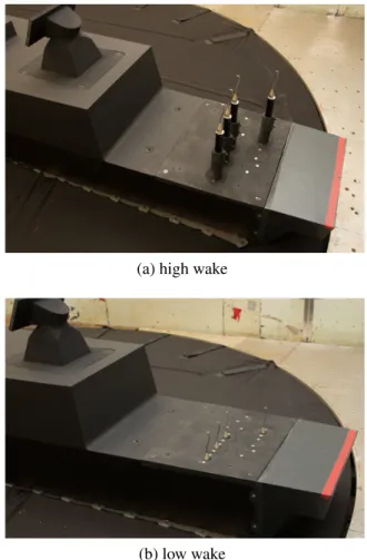
w is the normalized vertical component of flow speed. To illustrate the concepts in this paper, the air-wake characteristics of three sample points in the airwake of the GD for headwind conditions will be discussed as three cases, each with increasing order of magnitude of OOR level compared to the previous. Table 1 shows the cases, with coordinates as shown in Figure 3, and corresponding OOR levels. Case A represents a point near the edge of the deck which is exposed to largely unaffected air that flows around the superstructure. Case A has inconsequential OOR levels. Case B is in the lateral centre of the deck at the nominal height of a helicopter rotor plane in high hover. Case B is directly in the wake of the rotating radar feature on top of the hangar. Case B has mild OOR levels. Case C is below Case B, well within the wake region caused by the superstructure of the ship. Case C has high OOR levels. Figure 4 shows the experimental setup for Case A and B (top), and Case C (bottom).
4. Discussion 4.1. Clipping
Clipping is represented in the time-series pro-duced by the data reduction code as zeros for those instantaneous measurements that fall outside of the acceptance cone. The first 100 samples of normal-ized flow speed magnitude for Case C is shown in Figure 5; note the inverted time-series shown in the figure will be discussed later in the paper.
Statistical values, such as the mean and the root mean square (RMS) of the fluctuating component of the velocity signal, are commonly used for the
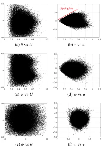
interpretation of flow data and also for the validation of CFD. Clipping affects these quantities because the time-series contain artificial zero values. However, the removal of the zeros prior to statistic calculation does not yield correct values either. To investigate the clipping phenomenon, scatter plots of U vs θ, U vs ψ, and θ vs ψ were created. One each plot, the value for each instantaneous measurement is a data point. The same was done for the orthogonal component system, with u vs v, u vs w, and v vs w. Figures 6, 7, and 8 show the results for Cases A, B, and C respectively.
For Case A, (Figure 6), the U vs ψ and θ vs ψ plots show minimal evidence of clipping in yaw. The u vs vplot shows the effect of clipping in the orthogonal component system, where a ∼1:1 clip line relating u and v illustrates the ratio of components correspond-ing to the yaw clippcorrespond-ing angle of ∼45◦. Other plots show a mainly round scatter shape with diffuse edges; this shape corresponds to normally distributed turbu-lence for that component.
Considering Cases B and C (Figures 7 and 8), the clipping lines at ∼45◦for θ and ψ in the left column appear more defined as the OOR rate increases. The clipping lines on u vs v and u vs w, which represent flow angles of ∼45◦, are also more pronounced. These plots suggest that the majority of clipped data points occur when the streamwise flow speed (u) is low, which leads to higher flow angles for typical values of the lateral and vertical velocity components.
No clipping lines are visible along the U axis or in the w vs v scatter plot, even though these time-series contain the same number of zeros as θ and ψ. This observation illustrates why the effects of clipping are difficult to quantify when the data is examined in certain ways.
Typically, the calculation of mean and RMS are important quantities used in the analysis of airwake data. However, for clipped signals, these statistical quantities can produce unreliable results. Even the exclusion of the zeros in the time-series leads to in-correct results because the clipping is not random, but rather systematically excludes measurements outside the acceptance cone. Table 2 shows the mean and RMS calculated with the zeros included (w/ 0) and excluded (w/o 0) in the calculation for all three cases.
Statistics for Cases A and B are similar with and without the zeros included since there are relatively
few zeros in the time-series. Case C, however, has significantly different values for both mean and RMS with and without zeros included in the calculation. Based on experience for ship airwake studies, an OOR rate of 0.05 is typically considered the limit for using calculated statistics directly before considering the effects of clipping.
Although all the values in Table 2 are subject to some degree of clipping, the comparison of the values with and without the zeros included provides insight into the sensitivity to clipping for different types of flows. This information is useful when considering the accuracy requirements for the interpretation of flow data for specific applications.
4.2. Effect of Clipping on Spectra
The flow spectra is another common quantity for the analysis of flow characteristics and for conducting CFD validation as discussed by Yuan et al. (2018). Since the temporal spacing between measurements is of importance for frequency-domain analysis, the re-moval of the zeros in the time-series leads to incorrect spectral information. The spectral magnitudes of the original signals cannot be used directly because the RMS values, equivalent to the square-root of the area under the spectra, are contaminated by clipping as discussed in previous sections. However, the original spectra could be used for validation of CFD if the CFD data were clipped in post-processing according to the physical phenomenon affecting the Cobra probe data.
To assess the impact of the presence of the clipped measurements on the spectra, the time-series was modified as follows:
• All original time-series measurements with zero values were assigned to value of “1”.
• All original time-series measurements with non-zero values were assigned the value of “0”. These modifications created an equivalent time-series where the frequency content is associated only with the act of switching between values inside and outside the acceptance cone. This time-series has been named the “inverted time-series”. Figure 5 shows this concept for the first 100 samples for Case C.
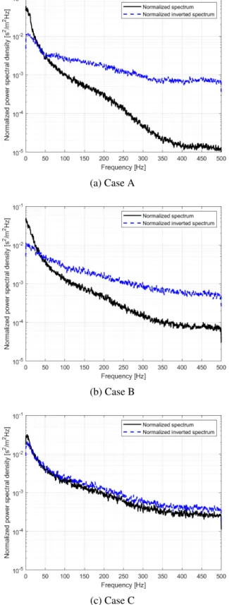
Figure 9 shows the comparison of the normalized power spectral density for Cases A, B, and C respec-tively starting from the top for both the original and the inverted time-series. The spectra are normalized by their individual variance values calculated with clipped zeros removed. Although the flow spectra are affected by the clipping phenomenon, comparing the spectral shapes for the original and the inverted time-series can provide some insight into the effect of clipping. Based on Figure 9, the clipping occurs across the full range of frequencies as opposed to at a single frequency or narrow frequency range. For Cases A and B, the inverted spectra are similar while for Case C the inverted spectra shows some degree of higher clipping at lower frequencies. This obser-vation suggests that there may be a systematic na-ture to the effect of clipping on the spectra. Further, the impact of clipping for different cases could be assessed by comparing the inverted spectra to one another. These ideas may be useful in the future for analysis of clipped data.
4.3. Probability Distributions
With the standard methods of flow analysis signif-icantly affected by clipping, probability distributions present another tool with noteworthy advantages. The concept of using probability distributions to analyze bluff body flows is presented by Roshko (1953).
A one-dimensional probability distribution e ffec-tively integrates along one axis of a scatter plot to create a histogram as shown in Figures 6 to 8. There-fore, only θ and ψ shows the effect of clipping, while the other quantities, U, u, v, and w, appear continu-ous even though they are missing data points. One-dimensional probability distributions are still some-what contaminated by the missing data points in the other angle axis, however they still provide insight into the clipping phenomenon.
The one-dimensional probably distributions of θ and ψ were calculated by finding the mean and RMS of the original time-series with the zeros removed and binning the individual time-series measurements into bins of width 1/50thof the RMS value. The number of data points in each bin were then normalized by the length of the original time-series (including zeros) and plotted to obtain the probability distribution. Fig-ure 10 shows the θ probability distributions for Cases
A, B, and C respectively starting from the top, and Figure 11 shows the ψ distributions. The effect of clipping is clearly seen in both θ and ψ for Case C, and can just be made out at the bottom of the distribu-tions for Case B. Although it is known that 0.3% of the measurements in the time-series for Case A are clipped and Figure 6 indicates that these primarily occur on the positive end of the yaw range, the dis-tribution does not clearly show the clipping for Case A.
Similar to the frequency domain analysis, valida-tion of CFD results can be done in the probability domain as shown by Yuan et al. (2018). For pitch and yaw, because the clipping is directly visible, the results can be compared without modifying the CFD data according to the acceptance cone. Comparisons for other components in the probability domain re-quire that the CFD data be modified.
The shapes of the distributions also give some insight into the flow itself, indeed many researchers have used to probability distributions of turbulence to analyze flow characteristics as described by Townsend (1947), Ferchichi and Tavoularis (2002), Davies (1966), and Frenkiel and Klebanoff (1973). Gaussian distribu-tions are typically characteristic of well-mixed wake flow whereas non-Gaussian shapes can indicate other wake features. The idea of using probability distribu-tions to analyze wake data is not new. To the authors’ knowledge, however, no comprehensive description of the correlation between probability shape and flow feature is available in the open literature. Separate to this paper, the authors hypothesize that the study of distribution shapes for different types of turbulence flows could lend new insight into the structure of tur-bulence for bluff body flows and also possibly a new tool for characterizing flow features. The authors be-lieve this would be a worthwhile addition to the body of knowledge in bluff body aerodynamics.
It can be seen in Figure 6 that the distributions of both θ and ψ for Case A are approximately Gaus-sian, indicating relatively well-mixed turbulence. The shape of the ψ distribution for Cases B, considering the location of the data, implies a lateral flapping shear layer or vortex shedding flow feature. Inter-estingly, although the data for Case B is nearest to the shear layer separating off the top of the super-structure, the flow features are dominated by lateral
flapping drive by the sides of the superstructure. The distributions for Case C also exhibit non-Gaussian trends.
4.4. Curve Fitting to Recover Statistics
Since the effect of clipping can clearly be seen in the probability domain and some flows are approxi-mately Gaussian, an attempt was made to recover re-liable mean and RMS statistics for those cases where the distributions are Gaussian. This approach enables easy CFD validation without the requirement to artifi-cially clip the CFD data.
The mathematical equation for a one-dimensional Gaussian distribution can sometimes be used to re-cover mean and RMS by curve-fitting to the data that is available. The Gaussian distribution for flow angle β is
φ(β) = ˆφ e−(β− ¯β)2/2 σβ2
(6) where,
φ is the Gaussian function of the flow angle β; β is one of the flow angles;
¯
β is the fitted mean (centre of the peak); σβ is the fitted RMS; and
ˆ
φ is the magnitude of the peak.
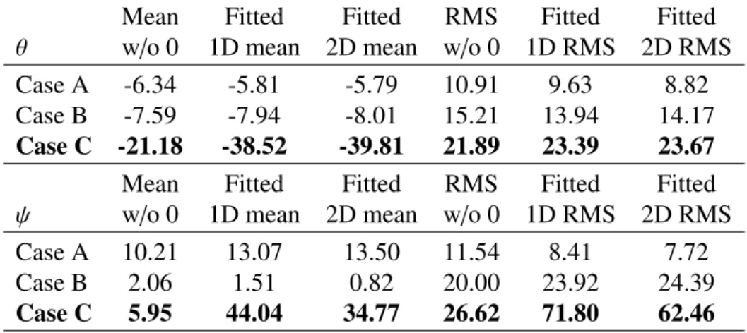
Equation 6 was fitted to the calculated probability distributions for Cases A, B, and C using a multi-dimensional unconstrained nonlinear minimization algorithm. The resulting fits were overlayed on the experimental data in Figures 10 and 11. The corre-sponding fitted mean and RMS of the flow angles are given in Table 3 and are compared to the values from Table 2 with zeros removed.
Currently, visual inspection is used to determine whether recovered statistical values are reliable; how-ever and algorithm to assess the quality of the Gaus-sian fit could likely be developed. By examining the fits compared to the experimental data, it can be seen that the distributions for θ for Cases A and B, and ψ for Case A are approximately, but not exactly Gaus-sian. Therefore, the fitted values differ somewhat
from the calculated values. The variation in values in Table 2 shows the sensitivity of the statistical values to minor deviations from a Gaussian distribution.
By inspection, the distributions for Case C and ψ for Case B are not fundamentally Gaussian in shape; therefore the recovered mean and RMS values can-not be considered an improvement over the calcu-lated statistics. The functional form of many different types of mathematical distributions were considered in an effort to find a more suitable for for these non-Gaussian cases. To date, no other distribution type that allows the recovery of the mean and RMS as part of the fitting process has been identified. Although the fitted quantities for highly non-Gaussian distributions cannot be reliably used for validation it in interest-ing to note that the fitted mean is within 0.5◦and the fitted RMS is within 4◦. Give the wide variation in flow features in bluff body flows, this accuracy may be sufficient to justify the use of fitted statistics for moderately clipped time-series depending on the ap-plication.
In examining θ distribution for Case C, the fixed pitch angle of the probe resulted in data collected where the mean flow angle (according to the distribu-tion) occurred near the edge of the acceptance cone range. The calculated mean value using the time-series with zeros removed was -21◦, which is sig-nificantly different than the fitted value of -38◦. Al-though the fitted value may be accurate only to within a handful of degrees, the fitted value is no doubt more appropriate than the calculated value in this case.
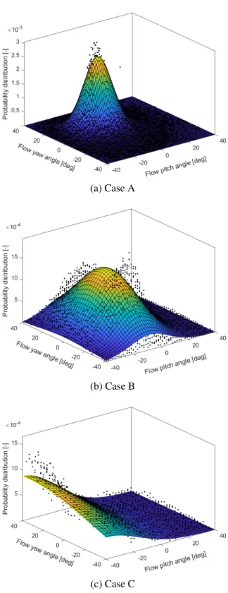
A two-dimensional Gaussian distribution for pitch, θ, and yaw, ψ, is
φ(θ, ψ) = ˆφ e−[(θ−¯θ)22 σθ2+ (ψ− ¯ψ)2
2 σψ2] (7)
where,
φ is the two-dimensional Gaussian function; θ,ψ are the flow angles;
¯
θ, ¯ψ are the fitted means (centre of the peak); σθ,σψ are the fitted RMS values; and
ˆ
Figure 12 shows the two-dimensional Gaussian fits for all three cases, with the fitted mean and RMS values shown in Table 2. For Cases A and B, the differences between the 1D and 2D fitted mean and RMS values is minimal. As discussed, the distribution shapes and their associated Gaussian fits, both one-and two-dimensional, are believed to offer insight into the understanding of qualitative flow characteristics. The study of the relationship between distributions and flow characteristics is the subject of future work. 5. Conclusions
This paper has explored the use of moderate to highly clipped Cobra probe data in the study of bluff body wakes and CFD validation. Since clipping con-taminates those quantities generally used for analysis, including mean, RMS of the fluctuating flow compo-nents, and spectra, the use of probability distributions is introduced as a useful tool. Because of the mecha-nism associated with the signal clipping, probability distributions of flow angles can be compared with clipped data directly, allowing validation of CFD data without modifying the CFD data to include the effect of clipping.
Probability distributions may also be useful to provide insight about the flow itself. Some flows exhibit largely Gaussian distributions, while others exhibit different shapes. Gaussian curve-fitting can be used to recover useful mean and RMS values for some highly clipped flows; however, this approach may have some limitations. The interpretation of different distribution shapes for different flow characteristics is a point of future study.
6. References
AVT-315 Research Task Group, 2017. Terms of reference: Com-parative assessment of modeling and simulation methods of shipboard launch and recovery of helicopters. North Atlantic Treaty Organisation.
Bell, J., Burton, D., Thompson, M., Herbst, A., Sheridan, J., 2016. Flow topology and unsteady features of the wake of a generic high-speed train. Journal of Fluids and Structures 61, 168–183.
Davies, P., 1966. Turbulence structure in free shear layers. AIAA Journal 4 (11), 1971–1978.
Ferchichi, M., Tavoularis, S., 2002. Scalar probability density function and fine structure in uniformly sheared turbulence. Journal of Fluid Mechanics 461, 155–182.
Frenkiel, F., Klebanoff, P., 1973. Probability distributions and correlations in a turbulent boundary layer. The physics of fluids 16 (6), 725–737.
Hanfeng, W., Yu, Z., Chao, Z., Xuhui, H., 2016. Aerodynamic drag reduction of an Ahmed body based on deflectors. Journal of Wind Engineering and Industrial Aerodynamics 148, 34– 44.
Hooper, J. D., Musgrove, A. R., 1997. Reynolds stress, mean velocity, and dynamic pressure measurement by a four-hole pressure probe. Experimental Thermal and Fluid Science 15, 375–383.
Mallipudi, S., Selig, M., Jun. 2004. Use of a four-hole Cobra probe to determine the unsteady wake characteristics of rotat-ing objects. In: AIAA Aerodynamic Measurement Technol-ogy and Ground Testing Conference. No. AIAA 2004-2299. Portland, Oregon, USA.
Owen, I., Lee, R., Wall, A., Fernandez, N., 2021. The NATO Generic Destroyer - a shared geometry for collaborative re-search into modelling and simulation of shipboard launch and recovery. Accepted to Ocean Engineering.
Roshko, A., Mar. 1953. On the development of turbulent wakes from vortex streets. Tech. Rep. Technical Note 2913, National Advisory Committee for Aeronautics.
Townsend, A., 1947. Measurements in the turbulent wake of a cylinder. In: The Royal Society A. Vol. 190. pp. 551–561. Wall, A., Lee, R., Barber, H., McTaggart, K., Feb. 2021. The
NATO Generic Destroyer - a shared geometry for collabo-rative research into modelling and simulation of shipboard launch and recovery: source data posting on Open Science Canada. Use title keywords at https: //open.canada.ca/en/open-data.
White, C., Lim, E., Watkins, S., Mohamed, A., Thompson, M., 2012. A feasibility study of micro air vehicles soaring tall buildings. Journal of Wind Engieering and Industrial Aerodynamics 103, 41–49.
Yuan, W., Wall, A., Lee, R., 2018. Combined numerical and ex-perimental simulations of unsteady ship airwakes. Computers and Fluids 172, 29–53.
Table 1: Flow measurement points for sample cases (coordinates in inches model scale). Position x(in) y(in) z(in) OOR
Case A top side 11.8 4.7 9.1 0.002 Case B top middle 11.8 0 9.1 0.024 Case C bottom middle 11.8 0 9.1 0.513
Table 2: Calculated Statistics. Mean Mean RMS RMS θ w/o 0 w/ 0 w/o 0 w/ 0 Case A -6.34 -6.34 10.91 10.92 Case B -7.59 -7.41 15.21 15.07 Case C -21.18 -10.33 21.89 18.60 Mean Mean RMS RMS ψ w/o 0 w/ 0 w/o 0 w/ 0 Case A 10.20 10.21 11.53 11.54 Case B 2.06 2.01 20.00 19.75 Case C 5.95 2.90 26.62 18.83
Table 3: Fitted statistics.
Mean Fitted Fitted RMS Fitted Fitted θ w/o 0 1D mean 2D mean w/o 0 1D RMS 2D RMS Case A -6.34 -5.81 -5.79 10.91 9.63 8.82 Case B -7.59 -7.94 -8.01 15.21 13.94 14.17 Case C -21.18 -38.52 -39.81 21.89 23.39 23.67 Mean Fitted Fitted RMS Fitted Fitted ψ w/o 0 1D mean 2D mean w/o 0 1D RMS 2D RMS Case A 10.21 13.07 13.50 11.54 8.41 7.72 Case B 2.06 1.51 0.82 20.00 23.92 24.39 Case C 5.95 44.04 34.77 26.62 71.80 62.46
Figure 1: Cobra probe.
Figure 2: Generic Destroyer model mounted in the 3 m × 6 m Propulsion and Icing Wind Tunnel.
Figure 3: Schematic representation of wake measure-ment points and coordinate systems (dimensions in inches model scale shown, full scale in brackets).
(a) high wake
(b) low wake
Figure 4: Instrument setup for measurements in the ship wake.
Figure 5: First 100 point of the time-series of nor-malized flow speed magnitude for point C and the corresponding inverted time-series.
(a) θ vs U (b) v vs u
(c) ψ vs U (d) w vs u
(e) ψ vs θ (f) w vs v
Figure 6: Scatter plots of flow properties for Case A. For each plot, caption shows vertical axis vs horizon-tal axis label.
(a) θ vs U (b) v vs u
(c) ψ vs U (d) w vs u
(e) ψ vs θ (f) w vs v
Figure 7: Scatter plots of flow properties for Case B. For each plot, caption shows vertical axis vs horizon-tal axis label.
(a) θ vs U (b) v vs u
(c) ψ vs U (d) w vs u
(e) ψ vs θ (f) w vs v
Figure 8: Scatter plots of flow properties for Case C. For each plot, caption shows vertical axis vs horizon-tal axis label.
(a) Case A
(b) Case B
(c) Case C
Figure 9: Comparison of normalized spectra for the clipped time-series of normalized flow speed magni-tude and the corresponding inverted time-series.
(a) θ for Case A
(b) θ for Case B
(c) θ for Case C
Figure 10: Probability distributions of θ with Gaus-sian fits overlayed.
(a) ψ for Case A
(b) ψ for Case B
(c) ψ for Case C
Figure 11: Probability distributions of ψ with Gaus-sian fits overlayed.
(a) Case A
(b) Case B
(c) Case C
Figure 12: Two-dimensional probability distributions with Gaussian fits overlayed.