The natural selection of words: finding the features of fitness

Publisher’s version / Version de l'éditeur:

Vous avez des questions? Nous pouvons vous aider. Pour communiquer directement avec un auteur, consultez la

première page de la revue dans laquelle son article a été publié afin de trouver ses coordonnées. Si vous n’arrivez

Questions? Contact the NRC Publications Archive team at

PublicationsArchive-ArchivesPublications@nrc-cnrc.gc.ca. If you wish to email the authors directly, please see the first page of the publication for their contact information.

https://publications-cnrc.canada.ca/fra/droits

L’accès à ce site Web et l’utilisation de son contenu sont assujettis aux conditions présentées dans le site LISEZ CES CONDITIONS ATTENTIVEMENT AVANT D’UTILISER CE SITE WEB.

PLoS ONE, 14, 1, 2019-01-28

READ THESE TERMS AND CONDITIONS CAREFULLY BEFORE USING THIS WEBSITE.

https://nrc-publications.canada.ca/eng/copyright

NRC Publications Archive Record / Notice des Archives des publications du CNRC : https://nrc-publications.canada.ca/eng/view/object/?id=78901fd2-32c0-4cd9-b524-68309ea681eb https://publications-cnrc.canada.ca/fra/voir/objet/?id=78901fd2-32c0-4cd9-b524-68309ea681eb

Archives des publications du CNRC

This publication could be one of several versions: author’s original, accepted manuscript or the publisher’s version. / La version de cette publication peut être l’une des suivantes : la version prépublication de l’auteur, la version acceptée du manuscrit ou la version de l’éditeur.

For the publisher’s version, please access the DOI link below./ Pour consulter la version de l’éditeur, utilisez le lien DOI ci-dessous.

https://doi.org/10.1371/journal.pone.0211512

Access and use of this website and the material on it are subject to the Terms and Conditions set forth at

The natural selection of words: finding the features of fitness

Turney, Peter D.; Mohammad, Saif M.

The natural selection of words: Finding the

features of fitness

Peter D. TurneyID1*, Saif M. Mohammad2*

1Ronin Institute, Montclair, New Jersey, United States of America, 2 National Research Council Canada, Ottawa, Ontario, Canada

*peter.turney@ronininstitute.org(PT);saif.mohammad@nrc-cnrc.gc.ca(SM)

Abstract

We introduce a dataset for studying the evolution of words, constructed from WordNet and the Google Books Ngram Corpus. The dataset tracks the evolution of 4,000 synonym sets (synsets), containing 9,000 English words, from 1800 AD to 2000 AD. We present a super-vised learning algorithm that is able to predict the future leader of a synset: the word in the synset that will have the highest frequency. The algorithm uses features based on a word’s length, the characters in the word, and the historical frequencies of the word. It can predict change of leadership (including the identity of the new leader) fifty years in the future, with an F-score considerably above random guessing. Analysis of the learned models provides insight into the causes of change in the leader of a synset. The algorithm confirms observa-tions linguists have made, such as the trend to replace the -ise suffix with -ize, the rivalry between the -ity and -ness suffixes, and the struggle between economy (shorter words are easier to remember and to write) and clarity (longer words are more distinctive and less likely to be confused with one another). The results indicate that integration of the Google Books Ngram Corpus with WordNet has significant potential for improving our understand-ing of how language evolves.

Introduction

Words are a basic unit for the expression of meanings, but the mapping between words and meanings is many-to-many. Many words can have one meaning (synonymy) and many mean-ings can be expressed with one word (polysemy). Generally we have a preference for one word over another when we select a word from a set of synonyms in order to convey a meaning, and generally one sense of a polysemous word is more likely than the other senses. These prefer-ences are not static; they evolve over time. In this paper, we present work on improving our understanding of the evolution of our preferences for one word over another in a set of synonyms.

The main resources we use in this work are the Google Books Ngram Corpus (GBNC) [1–

3] and WordNet [4,5]. GBNC provides us with information about how word frequencies change over time and WordNet allows us to relate words to their meanings.

a1111111111 a1111111111 a1111111111 a1111111111 a1111111111 OPEN ACCESS

Citation: Turney PD, Mohammad SM (2019) The

natural selection of words: Finding the features of fitness. PLoS ONE 14(1): e0211512.https://doi. org/10.1371/journal.pone.0211512

Editor: Richard A Blythe, University of Edinburgh,

UNITED KINGDOM

Received: October 31, 2018 Accepted: January 15, 2019

Published: January 28, 2019

Copyright:© 2019 Turney, Mohammad. This is an

open access article distributed under the terms of theCreative Commons Attribution License, which permits unrestricted use, distribution, and reproduction in any medium, provided the original author and source are credited.

Data Availability Statement: All files are available

from GitHub athttps://github.com/pdturney/ natural-selection-of-words.

Funding: The author(s) received no specific

funding for this work.

Competing interests: The authors have declared

GBNC is an extensive collection of word ngrams, ranging from unigrams (one word) to five-grams (five consecutive words). The ngrams were extracted from millions of digitized books, written in English, Chinese, French, German, Hebrew, Spanish, Russian, and Italian [1–3]. The books cover the years from the 1500s up to 2008. For each ngram and each year, GBNC provides the frequency of the given ngram in the given year and the number of books containing the given ngram in the given year. The ngrams in GBNC have been automatically tagged with part of speech information. Our experiments use the full English corpus, called

English Version 20120701.

WordNet is a lexical database for English [4,5]. Similar lexical databases, following the for-mat of WordNet, have been developed for other languages [6,7]. Words in WordNet are tagged by their parts of speech and by their senses. A fundamental concept in WordNet is the

synset, a set of synonymous words (words that share a specified meaning).

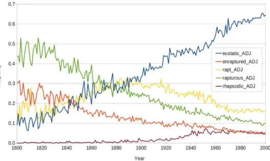
According to WordNet, ecstatic, enraptured, rapt, rapturous, and rhapsodic all belong to the same synset, when they are tagged as adjectives (enraptured could also be the past tense of the verb enrapture). They all mean “feeling great rapture or delight.” Based on frequency informa-tion from GBNC,Fig 1shows that rapturous was the most popular member of this synset from 1800 AD to about 1870 AD. After 1870, ecstatic and rapt competed for first place. By 1900,

ecstatic was the most popular member of the synset, and its lead over the competition

increased up to the year 2000. For convenience, we will refer to this as the rapturous–ecstatic synset.

Competition among words is analogous to biological evolution by natural selection. The leading word in a synset (the word with the highest frequency) is like the leading species in a genus (the species with the largest population). The number of tokens of a word in a corpus corresponds to the number of individuals of a species in an environment.

Brandon [8] states that the following three components are crucial to evolution by natural selection:

1. Variation: There is (significant) variation in morphological, physiological and behavioural

traits among members of a species.

2. Heredity: Some traits are heritable so that individuals resemble their relations more than they

resemble unrelated individuals and, in particular, offspring resemble their parents.

3. Differential Fitness: Different variants (or different types of organisms) leave different

num-bers of offspring in immediate or remote generations.

Godfrey-Smith [9] lists the same three components, calling them conditions for evolution by

natural selection.

When a system satisfies these three conditions, we have evolution by natural selection. Syn-sets satisfy the conditions. There is variation in the words in a synset: new words are coined and enter a synset, old words gain new meanings and enter a synset. There is heredity in word formation: this heredity is investigated in the field of etymology. There is differential fitness: some words become more popular over time and increase in frequency, other words become less popular and decline in frequency. Thus we may say that synsets evolve by natural selection.

Our focus in this paper is on differential fitness, also known as competition or selection. Selection determines which word will dominate (with respect to frequency or population) a synset. Here we do not attempt to model how new words are formed (variation) or how tokens are reproduced with occasional mutations (heredity), although these are interesting topics.

A number of recent papers have examined the problem of understanding how words change their meanings over time [10–13]. In contrast, we examine the problem of

understanding how meanings (synsets) change their words over time. Words compete to repre-sent a meaning, just as living organisms compete to survive in an environment. Regarding competition in biology, Darwin [14] wrote the following:

[. . .] it is the most closely allied forms—varieties of the same species and species of the same genus or of related genera—which, from having nearly the same structure, constitution, and habits, generally come into the severest competition with each other.

Likewise, the words in a synset, having nearly the same meaning, generally come into the severest competition with each other.

The project of understanding how synsets change their leaders raises a number of ques-tions: How much change is due to random events and how much is due to sustained pressures? What are the features of a word that determine its fitness for survival and growth in frequency? Is it possible to predict the outcome of a struggle for dominance of a synset?

We present an algorithm that uses supervised learning to predict the leading member of a synset, applying features based on a word’s length, its letters, and its corpus statistics. The algo-rithm gives insight into which features cause a synset’s leader to change.

The algorithm is evaluated with a dataset of 4,000 WordNet synsets, containing 9,000 English words and their frequencies in GBNC from 1800 AD to 2000 AD. The dataset enables us to study how English words have evolved over the last two hundred years. In this period, more than 42% of the 4,000 synsets had at least one change in leader. In a typical fifty-year interval, about 16.5% of the synsets experience a change in leader. The algorithm can predict leadership changes (including the identity of the new leader) fifty years ahead with an F-score of 38.5–43.3%, whereas random guessing yields an F-score of 17.3–24.8%.

The main contributions of this paper are (1) the creation and release of a dataset of 4,000 synsets containing a total of 9,000 English words and their historical frequencies [15], (2) a set of features that are useful for predicting change in the leader of a synset, (3) software for Fig 1. The normalized frequencies of the rapturous–ecstatic synset from 1800 AD to 2000 AD.The sum of the five frequencies for any given year is 1.0. The data has not been smoothed, in order to show the level of noise in the trends. This synset is typical with respect to the shapes of the curves and the level of noise in the trends, but it is atypical in that it contains more words than most of the synsets. Most of the synsets contain two to three words.

processing the dataset with supervised learning [15], generating models that can predict changes in synset leadership, (4) a method for analysis of the learned models that provides insight into the causes of changes in synset leadership.

In the next section, we discuss related work on evolutionary models of word change. The following section describes how we constructed the dataset of synsets and provides some statis-tics about the dataset. Next, we present the features that we use to characterize the dataset and we outline the learning algorithm. Four sets of experiments are summarized in the subsequent section. We then consider limitations and future work and present our conclusion.

Related work on the evolution of words

Much has been written about the evolution of words. Van Wyhe [16] provides a good survey of early research. Gray, Greenhill, and Ross [17] and Pagel [18] present thorough reviews of recent work. Mesoudi [19] gives an excellent introduction to work on the evolution of culture in general. In this section, we present a few relevant highlights from the literature on the evolu-tion of words.

Darwin believed that his theory of natural selection should be applied to the evolution of words [20]:

The formation of different languages and of distinct species, and the proofs that both have been developed through a gradual process, are curiously parallel. [. . .] The survival or preser-vation of certain favoured words in the struggle for existence is natural selection.

However, he did not attempt to work out the details of how words evolve.

Bolinger [21] argued that words with similar forms (similar spellings and sounds) should have similar meanings. As an example, he gave the words queen and quean, the latter meaning “a prostitute or promiscuous woman.” Bolinger claimed the word quean has faded away because it violates his dictum.

Magnus [22] defends the idea that some individual phonemes convey semantic qualities, which can be discovered by examining the words that contain these phonemes. For example, several words that begin with the letter b share the quality of roundness: bale, ball, bay, bead,

bell, blimp, blip, blob, blotch, bowl, bulb. We do not pursue this idea here, but we believe

resources such as GBNC and WordNet might be used to test this intriguing hypothesis. Petersen et al. [23] find that, as the vocabulary of a language grows, there is a decrease in the rate at which new words are coined. They observe that a language is like a gas that cools as it expands. Consistent with this hypothesis, we will show that, for English, the rate of change in the leadership of synsets has decreased over time.

Newberry et al. [24] examine three grammatical changes to quantify the strength of natural selection relative to random drift: (1) change in the past tense of 36 verbs, (2) the rise of do in negation in Early Modern English, and (3) a sequence of changes in negation in Middle English.

Cuskley et al. [25] study the competition between regular and irregular verbs. They find that the amount of irregularity is roughly constant over time, indicating that the pressures to make verbs conform to rules are balanced by counter-pressures. In our experiments below, we observe rivalries among various suffixes, indicative of similar competing pressures.

Ghanbarnejad et al. [26] analyze the dynamics of language change, to understand the vari-ety of curves that we see when we plot language change over time (as in ourFig 1). They intro-duce various mathematical models that can be used to gain a deeper understanding of these curves.

Amato et al. [27] consider how linguistic norms evolve over time. Their aim is to distin-guish spontaneous change in norms from change that is imposed by centralized institutions. They argue that these different sources of change have distinctive signatures that can be observed in the statistical data.

As we mentioned in the introduction, several papers consider how words change their meanings over time [10–13]. For example, Mihalcea and Nastase [10] discuss the shift in meaning of gay, from expressing an emotion to specifying a sexual orientation. Instead of studying how the meaning of a word shifts over time (same word, new meaning), we study how the the most frequent word in a synset shifts over time (same meaning, new word). As Darwin [20] put it, we seek to understand the “preservation of certain favoured words in the struggle for existence.”

Building datasets of competing words

Predicting the rise and fall of words in a synset could be viewed as a time series prediction problem, but we prefer another point of view. Fifty years from now, will ecstatic still dominate its synset, or will it perhaps be replaced by rapt? This is a classification problem, rather than a time series prediction problem. The classes are winner and loser.

Our algorithm has seven steps. The first four steps involve combining information from WordNet and GBNC to make an integrated dataset for studying the competition of words to represent meanings. The last three steps involve supervised learning with feature vectors. We present the first four steps in this section and the last three steps in the section Learning to

Model Word Change.

The first four steps yield a dataset that is agnostic about the feature vectors and algorithms that might be used to analyze the data. The first step extracts the frequency data we need from GBNC, the second step sums frequency counts for selected time periods, the third step groups words into synsets, and the fourth step splits the data into training and testing sets. The output of the fourth step is suitable for other researchers to use for evaluating their own feature vec-tors and learning algorithms. The results that other researchers obtain with this feature-agnos-tic dataset should be suitable for comparison with our results.

In the section Learning to Model Word Change, we take as input the feature-agnostic dataset that is the output of the fourth step. The fifth step adds features to the feature-agnostic data, the sixth step applies supervised learning, and the seventh step summarizes the results.

Past, present, and future

Imagine that the year is 1950 and we wish to predict which member of the rapturous–ecstatic synset will be dominant in 2000. In principle, we could use the entire history of the synset up to 1950 to make our prediction; however, it can be challenging to see a trend in such a large quantity of data.

To simplify the problem, we focus on a subset of the data. The idea is, to look fifty years into the future, we should look fifty years into the past, in order to estimate the pace of change. The premise is that this focus will result in a simple, easily interpretable model of the evolution of words.

We divide time into three periods, past, present, and future. Continuing our example, the

past is 1900, the present is 1950, and the future is 2000. Suppose that data from these three

peri-ods constitutes our testing dataset. We construct the training set by shifting time backwards by fifty years, relative to the testing dataset. In the training dataset, the past is 1850, the present is 1900, and the future is 1950. This lets us train the supervised classification system without peeking into our supposed future (the year 2000, as seen from 1950).

Integrating GBNC with WordNet

All words in WordNet are labeled with sense information. GBNC includes part of speech information, but it does not have word sense information. To bridge the word sense gap between GBNC and WordNet, we have chosen to restrict our datasets to the monosemous (single-sense) words in WordNet. A WordNet synset is included in our dataset only when every word in the synset is monosemous.

For example, rapt is represented in GBNC as rapt_ADJ, meaning the adjective rapt. We map the GBNC frequency count for rapt_ADJ to the WordNet representation rapt#a#1, mean-ing the first sense of the adjective rapt. We can do this because the adjective rapt has only one possible meaning, according to WordNet. If rapt_ADJ had two senses in WordNet, rapt#a#1 and rapt#a#2, then we would not know how to properly divide the frequency count of

rap-t_ADJ in GBNC over the two WordNet senses, rapt#a#1 and rapt#a#2.

The frequency counts in GBNC for the five words ecstatic_ADJ, enraptured_ADJ, rapt_ADJ,

rapturous_ADJ, and rhapsodic_ADJ are mapped to the five word senses ecstatic#a#1, enrap-tured#a#1, rapt#a#1, rapturous#a#1, and rhapsodic#a#1 in the rapturous–ecstatic synset in

WordNet. This is permitted because ecstatic_ADJ, enraptured_ADJ, rapt_ADJ, rapturous_ADJ, and rhapsodic_ADJ are all monosemous in WordNet.

The word enraptured could be either an adjective or the past tense of a verb. However, it is not ambiguous when it is tagged with a part of speech, enraptured_ADJ or enraptured_VERB. Thus we can map the frequency count for enraptured_ADJ in GBNC to the monosemous

enraptured#a#1 in WordNet.

There are other possible ways to bridge the word sense gap between GBNC and WordNet. We will discuss this in the section on future work.

Potential limitations of GBNC and WordNet

Before we explain how we combine GBNC and WordNet, we should discuss some potential issues with these resources. We argue that the design of our experiments mitigates these limitations.

The corpus we use, English Version 20120701, contains a relatively large portion of aca-demic and scientific text [28]. The word frequencies in this corpus are not representative of colloquial word usage. However, in our experiments, we only compare relative frequencies of words within a synset. The bias towards scientific text may affect a synset as a whole, but it is not likely to affect relative frequencies within a synset, especially since we restrict our study to monosemous words. The benefit of using English Version 20120701, compared to other more colloquial corpora, is its large size, which enables greater coverage of WordNet words and more robust statistical analysis.

Monosemous words tend to have lower frequencies than polysemous words, thus restrict-ing the study to monosemous words creates a bias towards lower frequency words. This could have a quantitative impact on our results. For example, lower frequency words may change more rapidly than higher frequency words, so the rate of change that we see with monosemous words may not be representative of what we would see with polysemous words. Even though this may have an impact on the specific numerical values we report, the same evolutionary mechanisms apply to both the monosemous and polysemous words, and thus the broader con-clusions on the trends reported here should be common to both.

In this study, we assume that WordNet synsets are stable over the period of time we con-sider, 1800 to 2000. Perc [29] argues that English evolved rapidly from 1520 to 1800 and then slowed down from 1800 to 2000. Although it is possible that WordNet synsets may be missing some words that were common around 1800, WordNet appears to have good coverage for the

last 200 years. Inspection of WordNet shows that it contains many archaic words that are rarely used today, such as palfrey and paltering.

Aside from potentially missing words, another possibility is that a word may have moved from one synset to another in the last 200 years. WordNet might indicate that such a word is monosemous and belongs only in the later synset. Although this is possible, we do not know of any cases where this has happened. It is likely that such cases are relatively rare and would have little impact on our conclusions.

Building datasets

We build our datasets for studying the evolution of words in four steps, as follows.

Step 1: Extract WordNet unigrams from GBNC. For the first sense of each unigram word in WordNet, if it contains only lower case letters and has at least three letters (for example,

ecsta-tic#a#1), then we look for the corresponding word in GBNC (ecstatic_ADJ) and find its

fre-quency for each year. GBNC records both the number of tokens of a word and the number of books that contain a word. By frequency, we mean the number of tokens. In Step 3, when we group words into synsets, we will eliminate synsets that contain words with a second sense (that is, words that are not monosemous). We believe that, if a synset contains a word that is not monosemous, then it is best to avoid the whole synset, rather than merely removing the polysemous word from the synset.

Step 2: Sum the frequency counts for selected time periods. GBNC has data extending from 1500 AD to 2008 AD, but the data is sparse before 1800. We sample GBNC for frequency information every fifty years from 1800 to 2000. To smooth the data, we take the sum of the frequency counts over an eleven-year interval. For example, for the year 1800, we take the sum of the frequency counts from 1795 to 1805; that is, 1800 ± 5. Frequency information from 1806 to 1844, from 1856 to 1894, and so on, is not used. (See the first column ofTable 1).

Step 3: Group words into synsets. Each synset must contain at least two words; otherwise there is no competition between words. Every word in a synset must be monosemous. If any word in a given synset has two or more senses, the entire synset is discarded.

Step 4: Split the data into training and testing sets. Each training or testing set covers exactly three time periods: past, present, and future. Each training set is shifted fifty years backward from its corresponding testing set. Given a sampling cycle of fifty years, from 1800 to 2000, we have two train–test pairs, as shown inTable 1. We remove a synset from a training or testing set if there is a tie for first place in the present or the future. We also remove a synset from a training or testing set if it contains any words that are unknown in the present. A word is con-sidered to be unknown in the present if it has a frequency of zero in the present. If a word’s Table 1. Time periods for the training and testing sets, given a fifty-year cycle of eleven-year samples.The average synset contains 2.23 to 2.25 words.

Period Train1 Test1 Train2 Test2

1800 ± 5 past

1850 ± 5 present past past

1900 ± 5 future present present past

1950 ± 5 future future present

2000 ± 5 future

Synsets 2,528 3,484 3,484 4,092

Words 5,640 7,795 7,795 9,198

Words per synset 2.23 2.24 2.24 2.25

Change 17.3% 19.0% 19.0% 13.3%

frequency in the present is zero, then it is effectively dead and it is not a serious candidate for being a future winner. We decided that including synsets that contain dead words would artifi-cially inflate the algorithm’s score.

The bottom rows ofTable 1give some summary statistics. Synsets is the number of synsets in each dataset and words is the number of words. Change is the percentage of synsets where the leader changed between the present and the future.

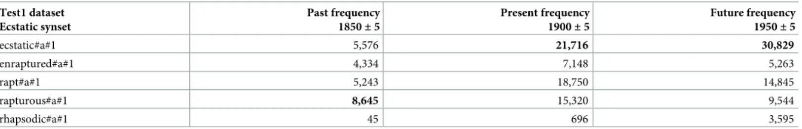
Table 2shows a sample of the output of Step 4. The sample is the entry for the rapturous–

ecstatic synset in the Test1 dataset. In 1850 (considered to be the past in Test1), rapturous was

the leading member of the synset. In 1900 and 1950 (considered to be the present and the future in Test1), ecstatic took over the leadership.

The amount of change in the datasets

A key question about how language evolves is how frequently the meanings have new leaders, and how this rate of leadership change itself changes over time.Table 3summarizes the amount of change, given a cycle of fifty years from 1800 to 2000, with word frequency counts summed over eleven-year intervals. Here we analyze the data after Step 3 and before Step 4. The table shows that 42% of the synsets had at least one change of leadership over the course of 200 years. Since only five periods are sampled (see the first column inTable 1), at most four changes are possible. The bottom row ofTable 3shows that two synsets experienced this maxi-mum level of churn.

The amount of change that we see depends on the cycle length (fifty years) and the interval for smoothing (eleven years). Shorter cycles and shorter smoothing intervals will show more change, but we should also expect to see more random noise. In the setup we have described in this section, we chose relatively long cycles and smoothing intervals, in an effort to minimize noise. By summing over eleven-year intervals and sampling over fifty-year intervals, we greatly reduce the risk of detecting random synset changes. On the other hand, we increase the risk that we are missing true synset changes. In our experiments, we will explore different cycle lengths.

Learning to Model Word Change

Now that we have training and testing datasets, we apply supervised learning to predict when the leadership of a synset will change. We do this in three more steps, as follows.

Step 5: Generate feature vectors for each word. We describe how we generate feature vectors for each word in the next section. Our final aim is to make predictions at the level of synsets. For example, given the past and present data for the rapturous–ecstatic synset in Test1 (see

Table 2), we want to predict that ecstatic will be the leader of the synset in the future. To make such predictions, we first work at the level of individual words, then we later move up to the synset level.

Step 6: Train and test a supervised learning system at the word level. For each word, we need a model that can estimate its future fitness; that is, the number of tokens the word will have in the future, relative to its competition (the other words in the synset). We treat this as a binary classification task, where the two classes are winner and loser. However, for Step 7, we need to estimate the probability of being a winner, rather than simply guessing the class. Later we will explain how we obtain probabilities. The probability of winning can be interpreted as the esti-mated future fitness of a word.

Step 7: Summarize the results at the synset level. Given probabilities for each of the words in the synset, we guess the winner by simply selecting the word with the highest probability of winning. Thus, for each synset, we have one final output: the member of the synset that we

expect to be the winner. The probabilities described in Step 6 are more useful for this step than the binary classes, winner and loser. Probabilities are unlikely to yield ties, whereas binary clas-ses could easily yield two or more winners or zero winners.

Feature vectors for words

We represent each word with a vector consisting of eight features and the target class. There are two length-based features, three character-based features, and four corpus-based elements (three features and the class). We will first define the features, then give examples of the vectors.

Feature 1: Normalized length is the number of characters in the given word, divided by the maximum number of characters for any word in the given synset. The idea is that shorter words might be more fit, since they can be generated with less effort. [length-based,

real-valued]

Feature 2: Syllable count is the number of syllables in the given word [30]. The intuition behind this feature is that normalized length applies best to written words, whereas syllable

count applies best to spoken words, so the two features may be complementary. [length-based, integer-valued]

Feature 3: Unique ngrams is the set of letter trigrams in the given word that are not shared with any other words in the given synset. This is not a single feature; it is represented by a high-dimensional sparse binary vector. The motivation for this feature vector is that there may be certain trigrams that enhance the fitness of a word. Before we split the given word into tri-grams, we add a vertical bar to the beginning and ending of the word, so that prefix and suffix trigrams are distinct from interior trigrams. For example, ecstatic becomes |ecstatic|, which yields the trigrams |ec, ecs, cst, sta, tat, ati, tic, and ic|. However, the trigram ic| is not unique to

ecstatic, since it is shared with rhapsodic. Likewise, rapturous shares its first four letters with rapt, so the unique trigrams for rapturous must omit |ra, rap, and apt. Also, overlap with enraptured means that ptu and tur are not unique to rapturous. The reason for removing

shared trigrams is that they cannot distinguish the winner from a loser; we want to focus on the features that are unique to the winner. [character-based, sparse binary vector]

Table 2. A sample of the Test1 dataset entries for the rapturous–ecstatic synset.The highest frequencies for each time period are marked in bold, indicating the winners. Test1 dataset Ecstatic synset Past frequency 1850 ± 5 Present frequency 1900 ± 5 Future frequency 1950 ± 5 ecstatic#a#1 5,576 21,716 30,829 enraptured#a#1 4,334 7,148 5,263 rapt#a#1 5,243 18,750 14,845 rapturous#a#1 8,645 15,320 9,544 rhapsodic#a#1 45 696 3,595 https://doi.org/10.1371/journal.pone.0211512.t002

Table 3. The frequency of synset leadership changes over 200 years, given a fifty-year cycle of eleven-year samples.

Change of leadership is common.

� N changes Number of synsets Percent of synsets

� 1 change 1,817 42.14%

� 2 changes 518 12.01%

� 3 changes 65 1.51%

= 4 changes 2 0.05%

Feature 4: Shared ngrams is the fraction of letter trigrams in the given word that are shared with other words in the given synset. A large fraction indicates that the given word is quite similar to its competitors, which might be either beneficial or harmful for the word.

[charac-ter-based, real-valued]

Feature 5: Categorial variations is the number of categorial variations of the given word. One word is considered to be a categorial variation of another word when the one word has been derived from the other. Often, but not always, the two words have different parts of speech. For example, hunger_NOUN, hunger_VERB, and hungry_ADJ are categorial variations of each other [31,32]. The calculation of categorial variations takes the birth date of a word into account; that is, the number of categorial variations of a word does not include variations that were unknown at the specified present time. A word with many categorial variations is analogous to a species with many similar species in its genus. This suggests that the ancestor of the species was highly successful [33]. [character-based, integer-valued]

Feature 6: Relative growth is the growth of a word relative to its synset. Suppose the word

ecstatic occurs n times in the present; that is, n is the raw frequency of ecstatic in the present.

Suppose the total of the raw frequencies of the six words in the rapturous–ecstatic synset is N. The relative frequency of ecstatic is n/N, the frequency of ecstatic relative to its synset. Let f1, f2,

and f3be a word’s relative frequencies in the past, present, and future, respectively. LetΔ be

rel-ative growth, the change in relrel-ative frequency from past to present,Δ = f2− f1. The relative

growth of ecstatic is its relative frequency in the present minus its relative frequency in the past.

If the synset as a whole is declining, the word in the synset that is declining most slowly will be growing relative to its synset. [corpus-based, real-valued]

Feature 7: Linear extrapolation is the expected relative frequency of the given word in the

future, calculated by linear extrapolation from the relative frequency in the past and the pres-ent. Since the time interval from past to present is the same as the time interval from present to future (fifty years), linear extrapolation leads us to expect the same amount of change from the present to the future; that is, f3= f2+Δ = 2f2− f1. [corpus-based, real-valued]

Feature 8: Present age is the age of the given word, relative to the present. We look in GBNC for the first year in which the given word has a nonzero frequency, and we take this year to be the birth year of the word. We then subtract the birth year from the present year, where the

pres-ent year depends on the given dataset. In Step 4, we require all words to have nonzero

frequen-cies in the present, so the birth year of a word is necessarily before the present year. The idea behind this feature is that older words should be more stable. [corpus-based, integer-valued]

Target class: The target class has the value 1 (winner) if the given word has the highest fre-quency in the given synset in the future, 0 (loser) otherwise. Ties were removed in Step 4, thus exactly one word in the given synset can have the value 1 for this feature. The class is the only element in the vector that uses future data, and it is only visible to the learning algorithm dur-ing traindur-ing. The time period that is the future in the traindur-ing data is the present in the testdur-ing data (seeTable 1). [corpus-based, binary-valued]

Table 4shows a sample of the output of Step 5. The sample displays the values of the ele-ments in the vectors for rapturous and ecstatic in the Test1 dataset. Unique ngrams is actually a vector with 3,660 boolean dimensions. Each dimension corresponds to a trigram. The four tri-grams that we see for rapturous inTable 4have their values set to 1 in the high-dimensional boolean vector. The remaining 3,656 trigrams have their values set to 0.

Supervised learning of probabilities

We use the naive Bayes classifier [34] in Weka [35,36] to process the datasets. Naive Bayes esti-mates the probabilities for the target class by applying Bayes’ theorem with the assumption

that the features are independent. We chose the naive Bayes classifier because it is fast, robust, it handles a variety of feature types, and the output model is easily interpretable.

The naive Bayes classifier in Weka has a number of options. We used the default settings, which apply normal (Gaussian) distributions to estimate probabilities. The data is split into two parts, feature vectors for which the class is 1 and feature vectors for which the class is 0. Each feature is then modeled by its mean and variance for each class value, assuming a Gauss-ian distribution. That is, we have two GaussGauss-ians for each feature.

Experiments with modeling change

This section presents four sets of experiments. The first experiment evaluates the system as described above; we call this system NBCP (Naive Bayes Change Prediction). The second experiment evaluates the impact of removing features from NBCP to discover which features are most useful. The third experiment varies the cycle length from thirty years to sixty years. The final experiment takes a close look at the model that is induced by the naive Bayes classi-fier, in an effort to understand what it has learned.

Experiments with NBCP

Table 1tells us that 19.0% of the synsets in Test1 and 13.3% of the synsets in Test2 undergo a change of leadership. In datasets like this, where there is a large imbalance in the classes (81.0– 86.7% in class 0 versus 13.3–19.0% in class 1), accuracy is not the appropriate measure of sys-tem performance. We are particularly interested in synsets where there is a change of leader-ship, but these synsets form a relatively small minority. Therefore, as our performance measures, we use precision, recall, and F-score for leadership change, as explained inTable 5.

The term changed inTable 5means that the present leader of the given synset is different from the future leader of the synset, whereas stable means that the present and future leader are the same. By right, we mean that the given algorithm correctly predicted the future leader of the synset, whereas wrong means that the given algorithm predicted incorrectly. True positive,

tp, is the number of synsets that experienced a change in leadership (changed) and the given Table 4. A sample of the Test1 vector elements for two of the five words in the rapturous–ecstatic synset.

Feature rapturous#a#1 ecstatic#a#1

Normalized length 0.900 0.800

Syllable count 3 3

Unique ngrams uro, rou, ous, us| |ec, ecs, cst, sta, tat, ati, tic

Shared ngrams 0.556 0.125 Categorial variations 3 2 Relative growth −0.122 0.107 Linear extrapolation 0.119 0.449 Present age 258 213 Target class 0 1 https://doi.org/10.1371/journal.pone.0211512.t004

Table 5. The 2 × 2 contingency table for change in the leadership of a synset.

Condition positive Condition nagative

Predicted positive True positive (tp) changed & right False positive (fp) stable & wrong Predicted negative False negative (fn) changed & wrong True negative (tn) stable & right

algorithm correctly predicted the new leader (right). The other terms, fp, fn, and tn, are defined analogously, by their cells inTable 5.

Now that we have the definitions of tp, fp, fn, and tn inTable 5, we can define precision,

recall, and F-score [37,38]:

precision¼ tp

tp þ fp ð1Þ

recall¼ tp

tp þ fn ð2Þ

F‐score ¼ 2 � precision� recall

precisionþ recall ð3Þ The F-score is the harmonic mean of precision and recall. For all three of the above equations, we use the convention that division by zero yields zero. The trivial algorithm that guesses there is never a change in leadership will have a tp count of zero, and therefore a precision, recall, and F-score of zero. On the other hand, the accuracy of this trivial algorithm would be 81.0– 86.7%, which illustrates why accuracy is not appropriate here.

Table 6shows the performance of the NBCP system on the two testing sets. With 3,484 syn-sets, the 95% confidence interval for the scores is ± 1.6%, calculated using the Wilson score interval [39]; thus the F-score for the NBCP system (38.5–43.3%) is significantly better than random guessing (17.3–24.8%), due to the much higher precision of the NBCP system, which compensates for the lower recall of NBCP, compared to random.

InTable 6, by random, we mean an algorithm that simulates probabilities by randomly selecting a real number from the uniform distribution over the range from zero to one. In Step 6, probabilities are calculated at the level of individual words, not at the level of synsets. Con-sider the synset {abuzz, buzzing}. The naive Bayes algorithm treats each of these words inde-pendently. When it considers abuzz, it does not know that buzzing is the only other choice. Therefore, when it assigns a probability to abuzz and another probability to buzzing, it makes no effort to ensure that the sum of these two probabilities is one. It only ensures that the proba-bility of abuzz being a winner in the future plus the probaproba-bility of abuzz being a loser in the future equals one. Our random system follows the same approach. For abuzz, it randomly selects a number from the uniform distribution over the range from zero to one, and this num-ber is taken as the probability that abuzz will be the winner. For buzzing, it randomly selects another number from the uniform distribution over the range from zero to one, and this is the Table 6. Various statistics for NBCP and random systems.All numbers are percentages, except for number of synsets.

Statistic Test1 Test2

Number of synsets 3,484 4,092

Percent changed 19.0 13.3

Percent stable 81.0 86.7

Precision for random 16.9 10.9

Recall for random 46.1 42.4

F-score for random 24.8 17.3

Precision for NBCP 51.0 47.3

Recall for NBCP 31.0 40.0

F-score for NBCP 38.5 43.3

probability that buzzing will be the winner. There is no attempt to ensure that these two simu-lated probabilities sum to one.

Feature ablation studies

Table 7presents the effect of removing a single feature from NBCP. The numbers report the F-score when a feature is removed minus the F-F-score with all features present. If every feature is contributing to the performance of the system, then we expect to see only negative numbers; removing any feature should reduce performance. Instead, we see positive numbers for syllable

count and unique ngrams, but these positive numbers are not statistically significant.

The numbers inTable 8report the F-score for each feature alone minus the F-score for ran-dom guessing. We expect only positive numbers, assuming every feature is useful, but there is one signficantly negative number, for shared ngrams in Test1.

Table 8shows that linear extrapolation is the most powerful feature. ComparingTable 7

withTable 8, we can see that the features mostly do useful work (Table 8), but their contribtion is hidden when the features are combined (Table 7). The comparison tells us that the features are highly correlated with each other.

Experiments with varying time periods

The NBCP system samples GBNC with a cycle of fifty years, as described above and shown in

Table 1. In this section, we experiment with cycles from thirty years up to sixty years.Table 9

reports the F-scores for the different cycle times. The dates given are for the future period of each testing dataset, since that is the target period for our predictions.

We have restricted our date range to the years from 1800 AD to 2000 AD, due to the spar-sity of GBNC before 1800 AD. We require a minimum of four cycles to build one training set and one testing set (see Train1 and Test1 inTable 1). With a sixty-year cycle, the four time periods that we use are 1820, 1880, 1940, and 2000. Only the final period, 2000, is both a future period and a testing period. With a seventy-year cycle, the four time periods would be 1790, 1860, 1930, and 2000. Therefore we prefer not to extend the cycle past sixty years.

Regarding periods shorter than thirty years, the amount of change naturally decreases as we shorten the cycle period. With less change, prediction could become more difficult.Table 10

shows how the amount of change varies with the cycle period.

ComparingTable 9withTable 10, we see that the F-score of random guessing declines as we approach the year 2000 (seeTable 9), following approximately the same pace as the decline of the percent of changed synsets (seeTable 10). On the other hand, the F-score of NBCP remains relatively steady; it is robust when the percent of changed synsets varies.

Table 7. The drop in F-score when a feature is removed from the NBCP system.Numbers that are statistically signif-icant with 95% confidence are marked in bold. Negative numbers indicate that a feature is making a useful contribu-tion to the system.

Feature Test1 Test2

Normalized length 0.00 −0.61 Syllable count 0.12 0.03 Unique ngrams −3.49 0.71 Shared ngrams 0.00 0.00 Categorial variations −0.07 −0.58 Relative growth −1.43 −0.76 Linear extrapolation −2.54 −10.08 Present age −0.19 −0.29 https://doi.org/10.1371/journal.pone.0211512.t007

In passing, we note thatTable 10suggests the amount of change is decreasing as we approach the year 2000. This confirms the analysis of Petersen et al. [23], mentioned in our discussion of related work.

Interpretation of the learned models

In this section, we attempt to understand what the learned models tell us about the evolution of words. For each feature, the naive Bayes classifier generates two Gaussian models, one for class 0 (loser) and one for class 1 (winner). Because naive Bayes assumes features are indepen-dent, we can analyze the models for each feature independently.

Here we are attempting to interpret the trained naive Bayes models, to gain insight into the role that the various features play in language change. Since the naive Bayes algorithm assumes the features are independent, the trained models cannot tell us anything about interactions among the features. It is likely that there are interesting interactions among the features. We leave the study of these interactions, possibly with algorithms such as logistic regression, for future work. For now, we focus on the individual impact of each feature.

Table 11shows the means of the Gaussians (the central peaks of the normal distributions) for the losers and the winners for each feature. This table omits unique ngrams, since it is a high-dimensional vector, not a single feature. We will analyze unique ngrams separately. The table only shows the models for Test1. Test2 follows the same general pattern.

Table 8. The F-score of each feature alone minus the F-score of random guessing.Numbers that are statistically sig-nificant with 95% confidence are marked in bold. Positive numbers indicate that a feature is better than random guessing.

Feature Test1 Test2

Normalized length 6.36 6.85 Syllable count 0.86 3.48 Unique ngrams 1.66 3.71 Shared ngrams −2.72 −0.08 Categorial variations −0.02 1.22 Relative growth 3.95 10.10 Linear extrapolation 9.62 23.49 Present age 5.01 5.52 https://doi.org/10.1371/journal.pone.0211512.t008

Table 9. The effect that varying cycle lengths has on the F-score of NBCP and random guessing.

Cycle Test1 Test2 Test3 Test4

30 years 1910 ± 5 1940 ± 5 1970 ± 5 2000 ± 5

F-score for NBCP 34.4 40.6 38.4 38.8

F-score for random 21.0 18.0 15.5 12.6

40 years 1920 ± 5 1960 ± 5 2000 ± 5

F-score for NBCP 34.7 38.3 42.5

F-score for random 22.7 19.0 16.1

50 years 1950 ± 5 2000 ± 5

F-score for NBCP 38.5 43.3

F-score for random 24.8 17.3

60 years 2000 ± 5

F-score for NBCP 39.5

F-score for random 21.2

The two length-based features, normalized length and syllable count, both tend to be lower for winning words. This confirms Bolinger’s [21] view that “economy of effort” plays a large role in the evolution of words; brevity is good. On the other hand, shared ngrams also tends to be lower, which implies that we prefer distinctive words. This sets a limit on brevity, since there is a limited supply of short words. Brevity is good, so long as words are not too similar.

We mentioned earlier that a word with many categorial variations is analogous to a species with many similar species in its genus, which may be a sign of success. This is supported by the naive Bayes model, since the winner has a higher mean for categorial variations than the loser.

The table shows that positive relative growth is better than negative relative growth and a high linear extrapolation is better than low, as expected. It also shows a high present age is good. In life, we tend to associate age with mortality, but present age is the age of a word type, not a token; it is analogous to the age of a species, not an individual. A species that has lasted for a long time has demonstrated its ability to survive.

Unique ngrams is a vector with 3,660 elements in Test1. To gain some insight into this

vec-tor, we sorted the elements in order of decreasing absolute difference between the mean of the Gaussian for class 0 and the mean for class 1.Table 12gives the top dozen trigrams with the largest gaps between the means. The size of the gap indicates the ability of the trigram to dis-criminate the classes. The difference column is the mean of the Gaussian of the winners (class 1) minus the mean of the Gaussian of the losers (class 0). When the difference is positive, the presence of the trigram in a word suggests that the word might be a winner. When the differ-ence is negative, the presdiffer-ence of the trigram in a word suggests that the word might be a loser.

Before splitting a word into trigrams, we added a vertical bar to the beginning and end of the word, to distinguish prefix and suffix trigrams from interior trigrams. Therefore the tri-gram ty| inTable 12refers to the suffix -ty.

In the table, we see that a high value for ty| or ity indicates a winner, but it is better to have low values for nes, ss|, and ess. Thus the naive Bayes model has confirmed the conflict between the suffixes -ity and -ness [40]: “Rivalry between the two English nominalising suffixes -ity and -ness has long been an issue in the literature on English word-formation.” Furthermore, the naive Bayes model suggests that -ness is losing the battle to -ity.

We also see that ize, ze|, and liz are indicative of a winner, whereas ise, se| and lis suggest a loser. There is a trend to replace the suffix -ise with -ize. This is known as Oxford spelling, although it is commonly believed (incorrectly) that the -ize suffix is an American innovation [41].

Table 10. The effect that varying cycle lengths has on the percentage of synsets that have changed leadership from present to future.

Cycle Test1 Test2 Test3 Test4

30 years 1910 ± 5 1940 ± 5 1970 ± 5 2000 ± 5 Percent changed 14.7 13.7 11.0 8.4 Number of synsets 3,041 3,622 3,958 4,275 40 years 1920 ± 5 1960 ± 5 2000 ± 5 Percent changed 17.5 14.5 11.0 Number of synsets 3,038 3,732 4,203 50 years 1950 ± 5 2000 ± 5 Percent changed 19.0 13.3 Number of synsets 3,484 4,092 60 years 2000 ± 5 Percent changed 15.4 Number of synsets 3,958 https://doi.org/10.1371/journal.pone.0211512.t010

It is interesting to see that the trigram ic| suggests a winner, and ecstatic eventually became the leader of the rapturous–ecstatic synset (seeFig 1). We looked in the Test1 unique ngrams vector for ous and found that the presence of ous suggests a loser. This may explain why ecstatic eventually won out over rapturous. However, we then need to explain the poor performance of

rhapsodic (seeFig 1). Looking again in the Test1 unique ngrams vector, the trigram dic suggests a loser, whereas the trigram tic suggests a winner. Although this is consistent with the success of ecstatic and the failure of rhapsodic, it is not clear to us why -tic should be preferred over -dic, given the apparent similarity of these suffixes.

Future work and limitations

Throughout this work, our guiding principle has been simplicity, based on the assumption that the evolution of words is a complex, noisy process, requiring a simple, robust approach to modeling. Therefore we chose a classification-based analysis, instead of a time series prediction algorithm, and a naive Bayes model, instead of a more complex model. The success of our approach is encouraging, and it suggests there is more signal and structure in the data than we expected. We believe that more sophisticated analyses will reveal interesting phenomena that our simpler approach has missed.

Table 11. Analysis of the naive Bayes models for Test1.The difference column is the mean of the Gaussian of the winners (class 1) minus the mean of the Gaussian of the losers (class 0). Differences that are statistically significant are marked in bold. Significance is measured by a two-tailed unpaired t test with a 95% confidence level. This table omits unique ngrams, which are presented in the next table.

Feature Means of Gaussians Mean of the winners is . . . Losers Winners Difference

Normalized length 0.9128 0.9087 −0.0041 lower

Syllable count 3.2494 3.2077 −0.0417 lower

Shared ngrams 0.4797 0.4726 −0.0071 lower

Categorial variations 3.3075 3.4432 0.1357 higher

Relative growth −0.0012 0.0956 0.0968 higher

Linear extrapolation 0.2058 0.8408 0.6350 higher

Present age 130.0 180.5 50.5 higher

https://doi.org/10.1371/journal.pone.0211512.t011

Table 12. Analysis of the unique ngrams features in the naive Bayes models for Test1.The table lists the top dozen trigrams with the greatest separation between the means. Differences that are statistically significant are marked in bold; all of the differences are significant. Significance is measured by a two-tailed unpaired t test with a 95% confidence level.

Trigrams Means of Gaussians Presence of the trigram suggests . . . Losers Winners Difference

ize 0.0055 0.0285 0.0230 winner ise 0.0289 0.0083 −0.0206 loser nes 0.0328 0.0134 −0.0194 loser ty| 0.0112 0.0297 0.0185 winner ss| 0.0379 0.0202 −0.0177 loser ity 0.0100 0.0269 0.0169 winner ze| 0.0022 0.0174 0.0152 winner ess 0.0373 0.0229 −0.0144 loser se| 0.0206 0.0083 −0.0123 loser lis 0.0154 0.0032 −0.0122 loser ic| 0.0228 0.0348 0.0120 winner liz 0.0022 0.0115 0.0093 winner https://doi.org/10.1371/journal.pone.0211512.t012

In particular, there is much room for more features in the feature vectors for words. We used three types of features: length-based, character-based, and corpus-based. There are most likely other types that we have overlooked, and other instances within the three types. We did a small experiment with phonetic spelling, using the International Phonetic Alphabet, but we did not find any benefit.

As we said in the introduction, the focus of this paper is selection. Future work should con-sider also variation and heredity, the other two components of Darwinian evolution. There is some past work on predicting variation of words [42].

This general framework may be applicable to other forms of cultural evolution. For exam-ple, the market share of a particular brand within a specific type of product is analogous to the frequency of a word within a synset. The fraction of votes for a political party in a given coun-try is another example.

As we discussed earlier in this paper, to bridge the gap between GBNC and WordNet, we restrict our datasets to the monosemous words in WordNet. Another strategy would be to allow polysemous words, but map all GBNC frequency information for a word to the first sense of the word in WordNet. That is, a synset would be allowed to include words that are not monosemous, but we would assign a frequency count of zero to all senses other than the first sense.

WordNet gives a word’s senses in order of decreasing frequency [4]. In automatic word sense disambiguation, a standard baseline is to simply predict the most frequent sense (the first sense) for every occurrence of a word. This baseline is difficult to beat [43]. This could be used as an argument in support of assigning a frequency count of zero to all senses other than the first sense, as a kind of first-order approximation.

We did a small experiment with this strategy, predicting the most frequent sense for every occurrence of a word. Our dataset expanded from 4,000 synsets containing 9,000 English words to 9,000 synsets containing 22,000 English words. The system performance was numeri-cally different but qualitatively the same as the results we reported above. However, we prefer to take the more conservative approach of only allowing monosemous words, since it does not require us to us to assume that we can ignore the impact of secondary senses on the evolution of a synset. The ideal solution to bridging the gap between GBNC and WordNet would be to automatically sense-tag all of the words in GBNC, but this would involve a major effort, requir-ing the cooperation of Google.

In the section on related work, we mentioned past research concerned with how words change their meanings over time (same word, new meaning) [10–13]. Let’s call this

meaning-change. Our focus in this paper has been how meanings change their words over time (same

meaning, new word; same synset, new leader). Let’s call this word-change. These two types of events, meaning-change and word-change, are interconnected.

Consider the case of a word that has two possible senses, and thus belongs to two different synsets. Suppose that the word’s dominant meaning has shifted over time from the first sense to the second sense, which is a case of meaning-change. If the frequency of the word in the first synset becomes sufficiently low and the frequency of the word in the second synset becomes sufficiently hight, then the word will be less likely to cause a reader or listener to be confused when it is used in the second sense. The meaning-change makes the word less ambig-uous and thus it becomes a better candidate for expressing the meaning of the second synset. This meaning-change may therefore cause a word-change. The leader of the second synset might be replaced by the less ambiguous candidate word.

This example illustrates how meaning-change might cause word-change. We can also imag-ine how word-change can cause meaning-change. We expect that future work will take an integrated approach to these two types of change. If the words in GBNC were automatically

sense-tagged, it would greatly facilitate this line of research. Here we have alleviated the issue of meaning-change and its impact on word-change by restricting our dataset to monosemous words. However, we have not completely avoided the issue of meaning-change, since monose-mous words can have shifts in connotations. There may also be shifts in meanings that Word-Net synsets do not capture. We have avoided precisely defining the relation between meaning-change and word-meaning-change, leaving this for future work, since there are multiple reasonable ways to define these terms and their relations.

Conclusion

This work demonstrates that change in which word dominates a synset is predictable to some degree; change is not entirely random. It is possible to make successful predictions several decades into the future. Furthermore, it is possible to understand some of the causes of change in synset leadership.

Of the various features we examined, the most successful is linear extrapolation. From an evolutionary perspective, this indicates that there is a relatively constant direction in the natu-ral selection of words. The same selective pressures are operating over many decades.

We observed that English appears to be cooling; the rate of change is decreasing over time. This might be due to a stable environment, as suggested by Petersen et al. [23]. It might also be due to the growing number of English speakers, which could increase the inertia of English.

This project is based on a fusion of the Google Books Ngram Corpus with WordNet. We believe that there is great potential for more research with this combination of resources.

This line of research contributes to the sciences of evolutionary theory and computational linguistics, but it may also lead to practical applications in natural language generation and understanding. Evolutionary trends in language are the result of many individuals, making many decisions. A model of the natural selection of words can help us to understand how such decisions are made, which will enable computers to make better decisions about language use.

Acknowledgments

We thank the PLOS ONE reviewers for their careful and helpful comments on our paper.

Author Contributions

Conceptualization:Peter D. Turney, Saif M. Mohammad.

Data curation:Peter D. Turney.

Formal analysis:Peter D. Turney.

Investigation:Peter D. Turney, Saif M. Mohammad.

Methodology:Peter D. Turney, Saif M. Mohammad.

Software:Peter D. Turney.

Writing – original draft:Peter D. Turney.

Writing – review & editing:Peter D. Turney, Saif M. Mohammad.

References

1. Michel JB, Shen YK, Aiden A, Veres A, Gray M, Pickett J, et al. Quantitative analysis of culture using millions of digitized books. Science. 2011; 331:176–182.https://doi.org/10.1126/science.1199644

2. Google. Google books ngram corpus; 2012. Available from:http://storage.googleapis.com/books/ ngrams/books/datasetsv2.html.

3. Google. Google books ngram viewer; 2013. Available from:https://books.google.com/ngrams/.

4. Fellbaum C, editor. Wordnet: An Electronic Lexical Database. Cambridge, MA: MIT Press; 1998.

5. WordNet. WordNet: A lexical database for English; 2007. Available from:https://wordnet.princeton.edu/

.

6. Vossen P. EuroWordNet: A multilingual database for information retrieval. In: Proceedings of the DELOS workshop on Cross-language Information Retrieval; 1997.

7. Vossen P. EuroWordNet: Building a multilingual database with wordnets for several European lan-guages; 2001. Available from:http://projects.illc.uva.nl/EuroWordNet/.

8. Brandon R. Concepts and methods in evolutionary biology. Cambridge, UK: Cambridge University Press; 1996.

9. Godfrey-Smith P. Conditions for evolution by natural selection. The Journal of Philosophy. 2007; 104:489–516.https://doi.org/10.5840/jphil2007104103

10. Mihalcea R, Nastase V. Word epoch disambiguation: Finding how words change over time. In: Proceed-ings of the 50th Annual Meeting of the Association for Computational Linguistics; 2012. p. 259–263.

11. Mitra S, Mitra R, Maity S, Riedl M, Biemann C, Goyal P, et al. An automatic approach to identify word sense changes in text media across timescales. Natural Language Engineering. 2015; 21(5):773–798.

12. Xu Y, Kemp C. A computational evaluation of two laws of semantic change. In: Proceedings of the 37th Annual Meeting of the Cognitive Science Society; 2015. p. 2703–2708.

13. Hamilton W, Leskovec J, Jurafsky D. Diachronic word embeddings reveal statistical laws of semantic change. In: Proceedings of the 54th Annual Meeting of the Association for Computational Linguistics; 2016. p. 1489–1501.

14. Darwin C. On the Origin of Species. London, UK: Penguin; 1968.

15. Turney P, Mohammad S. The natural selection of words: Software and guide to resources; 2019. Avail-able from:https://github.com/pdturney/natural-selection-of-words.

16. van Wyhe J. The descent of words: Evolutionary thinking 1780-1880. Endeavour. 2005; 29(3):94–100.

https://doi.org/10.1016/j.endeavour.2005.07.002PMID:16098591

17. Gray R, Greenhill S, Ross R. The pleasures and perils of Darwinizing culture (with phylogenies). Biolog-ical Theory. 2007; 2(4):360–375.https://doi.org/10.1162/biot.2007.2.4.360

18. Pagel M. Human language as a culturally transmitted replicator. Nature Reviews Genetics. 2009; 10:405–415.https://doi.org/10.1038/nrg2560PMID:19421237

19. Mesoudi A. Cultural Evolution. Chicago, IL: University of Chicago Press; 2011.

20. Darwin C. The Descent of Man. London, UK: Gibson Square; 2003.

21. Bolinger D. The life and death of words. The American Scholar. 1953; 22(3):323–335.

22. Magnus M. What’s in a Word? Studies in Phonosemantics. Norwegian University of Science and Tech-nology. Trondheim, Norway; 2001.

23. Petersen A, Tenenbaum J, Havlin S, Stanley E, Perc M. Languages cool as they expand. Scientific Reports. 2012; 2(943).

24. Newberry M, Ahern C, Clark R, Plotkin J. Detecting evolutionary forces in language change. Nature. 2017; 551:223–226.https://doi.org/10.1038/nature24455PMID:29088703

25. Cuskley C, Pugliese M, Castellano C, Colaiori F, Loreto V, Tria F. Internal and external dynamics in lan-guage: Evidence from verb regularity in a historical corpus of English. PLOS ONE. 2014; 9(8).https:// doi.org/10.1371/journal.pone.0102882PMID:25084006

26. Ghanbarnejad F, Gerlach M, Miotto J, Altmann E. Extracting information from S-curves of language change. Journal of The Royal Society Interface. 2014; 101.

27. Amato R, Lacasa L, Dı´az-Guilera A, Baronchelli A. The dynamics of norm change in the cultural evolu-tion of language. Proceedings of the Naevolu-tional Academy of Sciences. 2018; 115(33):8260–8265.https:// doi.org/10.1073/pnas.1721059115

28. Pechenick E, Danforth C, Dodds P. Characterizing the Google Books Corpus: Strong limits to infer-ences of socio-cultural and linguistic evolution. PLOS ONE. 2015.https://doi.org/10.1371/journal.pone. 0137041PMID:26445406

29. Perc M. Evolution of the most common English words and phrases over the centuries. Journal of the Royal Society Interface. 2012.https://doi.org/10.1098/rsif.2012.0491

30. Bowers N, Fast G. Lingua::EN::Syllable; 2016. Available from:https://metacpan.org/pod/Lingua::EN:: Syllable.

31. Habash N, Dorr B. A categorial variation database for English. In: Proceedings of HLT-NAACL 2003; 2003. p. 17–23.

32. Habash N, Dorr B. Catvar2.1: Categorial variation database for English; 2013. Available from:https:// clipdemos.umiacs.umd.edu/catvar/download.html.

33. Hunt T, Bergsten J, Levkanicova Z, Papadopoulou A, John OS, Wild R, et al. A comprehensive phylog-eny of beetles reveals the evolutionary origins of a superradiation. Science. 2007; 318(5858):1913– 1916.https://doi.org/10.1126/science.1146954PMID:18096805

34. John G, Langley P. Estimating continuous distributions in Bayesian classifiers. In: Eleventh Conference on Uncertainty in Artificial Intelligence. San Mateo: Morgan Kaufmann; 1995. p. 338–345.

35. Witten I, Frank E, Hall M, Pal C. Data Mining: Practical Machine Learning Tools and Techniques. San Francisco, CA: Morgan Kaufmann; 2016.

36. Weka. Weka 3: Data mining software in Java; 2015. Available from:https://www.cs.waikato.ac.nz/ml/ weka/.

37. van Rijsbergen C. Information Retrieval. London, UK: Butterworths; 1979.

38. Lewis D. Evaluating and optimizing autonomous text classification systems. In: Proceedings of the 18th Annual International ACM SIGIR Conference on Research and Development in Information Retrieval. ACM; 1995. p. 246–254.

39. Newcombe R. Two-sided confidence intervals for the single proportion. Statistics in Medicine. 1998; 17 (8):857–872.https://doi.org/10.1002/(SICI)1097-0258(19980430)17:8%3C857::AID-SIM777%3E3.0. CO;2-EPMID:9595616

40. Arndt-Lappe S. Analogy in suffix rivalry: The case of English -ity and -ness. English Language and Lin-guistics. 2014; 18(3):497–548.

41. Wikipedia. Oxford spelling; 2018. Available from:https://en.wikipedia.org/wiki/Oxford_spelling.

42. Skousen R. Analogy and Structure. New York, NY: Springer; 1992.

43. Hawker T, Honnibal M. Improved Default Sense Selection for Word Sense Disambiguation. In: Pro-ceedings of the 2006 Australasian Language Technology Workshop; 2006. p. 11–17.