Algorithms for transform selection in multiple-transform video compression

Algorithms for Transform Selection in

Multiple-Transform Video Compression

MASSACHUSETTS INSTITUTE

by

JUL

0

1 2012

Xun Cai

LIBRARIES

S.B. EE, University of Science and Technology of China, 2010

ARCHIVES

Submitted to the Department of Electrical Engineering and Computer

Science

in partial fulfillment of the requirements for the degree of

Master of Science in Electrical Engineering and Computer Science

at the

MASSACHUSETTS INSTITUTE OF TECHNOLOGY

June 2012

@

Massachusetts Institute of Technology 2012. All rights reserved.

Author ...

..

...

...

Department of Electrical Engineering and Computer Science

May 16, 2012

f

Certified b

ProfessoYJae S. Lim

Thesis Supervisor

Accepted by ...

. . . . .

Pr fess4jk4slie A. Kolodziejski

Chairman, Department Committee on Graduate Students

Algorithms for Transform Selection in Multiple-Transform

Video Compression

by

Xun Cai

Submitted to the Department of Electrical Engineering and Computer Science on May 16, 2012, in partial fulfillment of the

requirements for the degree of

Master of Science in Electrical Engineering and Computer Science

Abstract

Selecting proper transforms for video compression has been based on the rate-distortion criterion. Transforms that appear reasonable are incorporated into a video coding sys-tem and their performance is evaluated. This approach is tedious when a large num-ber of transforms are used. A quick approach to evaluate these transforms is based on the energy compaction property. With a proper transform, an image or motion-compensated residual can be represented quite accurately with a small fraction of the transform coefficients. This is referred to as the energy compaction property. How-ever, when multiple transforms are used, selecting the best transform for each block that leads to the best energy compaction is difficult.

In this thesis, we develop two algorithms to solve this problem. The first algorithm, which is computationally simple, leads to a locally optimal solution. The second algorithm, which is more intensive computationally, gives a globally optimal solution. We provide a detailed discussion on the ideas and steps of the algorithms, followed by the theoretical analysis of the performance. We verify that these algorithms are useful in a practical setting, by comparing and showing the consistency with rate-distortion results from previous research.

We apply the algorithms when a large number of transforms are used. These transforms are equal-length 1D-DCTs in 4x4 blocks, which try to characterize as many 1D structures as possible in motion-compensation residuals. By evaluating the energy compaction property of up to 245 transforms, we quickly determine whether these transforms will bring potential performance increase in a video coding system.

Thesis Supervisor: Professor Jae S. Lim Title: Professor of Electrical Engineering

Acknowledgments

First of all, I would like to express my sincere gratitude to my research advisor,

Professor Jae Lim, for his support and guidance during my M.S. research. His group provides me a chance to explore the research topic that interests me. His immense knowledge and vision helps me better understand the signal processing world. His constructive feedbacks, encouragement and patience have a remarkable influence on the completion of this thesis.

I would like to thank all the members that I have worked with in ATSP. Harley Zhang has provided a lot of technical help when I joined the group. Gun Bang has discussed both the research and general video processing technologies with me. I feel grateful for Cindy LeBlanc, who provides all kinds of support during my stay in this

group.

Finally, I would like to thank my family members in China. My parents financially supported me during my first semester at MIT, which allows me to settle down in my dream school. I am grateful for my fiancee and soulmate, Mengyu Zhang, who supports my career and respects my choice of life style.

Contents

1 Introduction

13

1.1 Energy Compaction ... ... 13

1.2 Evaluating the Energy Compaction in Multiple-Transform Environment 17 1.3 Overview of Thesis . . . . 20

2 Previous Research 21 2.1 Direction-Adaptive 1D DCTs . . . . 21

2.2 Rate-Distortion Performance of 1D-DCTs . . . . 24

2.3 Motivation for Thesis . . . . 25

3 Algorithms 27 3.1 Problem Formulation . . . . 28

3.2 A lgorithm A . . . . 29

3.2.1 Algorithm Description . . . . 29

3.2.2 Convergence . . . . 31

3.2.3 Initial Conditions and Local Convergence . . . . 32

3.2.4 Computational Complexity . . . . 34

3.3 A lgorithm B . . . . 35

3.3.1 Algorithm Description . . . . 35

3.3.2 Global Optimality . . . . 42

3.3.3 The difficulty of specifying the total number of coefficients . . 42

3.3.4 Computational Complexity . . . . 43

4 Simulations 45

4.1 Implementation and Experimental Setup . . . . 45

4.2 Algorithm Performance . . . . 47

4.2.1 Number of iterations required in Algorithm A . . . . 47

4.2.2 Initial conditions of Algorithm A . . . . 48

4.2.3 Quality of the locally optimal solutions obtained by Algorithm A 49 4.3 Comparison with R-D Performance . . . . 50

5 Applications: Evaluating the Energy Compaction for Equal-Length 1D-DCTs ₅₅ 5.1 Designs of Equal-Length 1D-DCTs . . . . 55

5.2 Overall Performance . . . . 58

5.3 Using all equal-length 1D-DCTs . . . . 61

5.4 Using part of equal-length 1D-DCTs . . . . 65

5.5 Conclusions . . . . 66

6 Conclusions 69 6.1 Sum m ary . . . . 69

List of Figures

1-1 Example of the energy compaction property of DCT . . . . 14

1-2 An example of 2D-DCT and energy compaction property. . . . . 16

1-3 An example of energy preservation computation with single block trans-form . . . . 18

1-4 An example of a typical image and motion compensated residual. . . 19

2-1 Sixteen 1D-DCTs of block size 8x8 . . . . 23

2-2 Eight 1D-DCTs of block size 4x4 . . . . 23

3-1 An example for iteration process of Algorithm A. . . . . 31

3-2 Graphical illustration of the iteration process of Algorithm A . . . . . 33

3-3 An example of computing the block optimal energy function . . . . . 36

3-4 Illustration of thresholding the incremental energy . . . . 38

3-5 Illustration of minimizing the cost function . . . . 40

3-6 Modification of the non-concave block optimal energy function . . . . 41

4-1 Source image used in simulations: QCIF sequence (resolution 177 x 144) MC residual "foreman" . . . . 46

4-2 Preserved energy in the first, second iterations and after convergence 48 4-3 Preserved energy with different initial conditions . . . . 49

4-4 Preserved energy of Algorithm A and Algorithm B . . . . 50

4-5 Preserved energy with different transform sets . . . . 52

5-1 All possible structures used in 4x4 equal-length transforms . . . . 57

5-3 Preserved energy of Algorithm A and Algorithm B . . . . 59 5-4 Frequencies for selection of transforms . . . . 60 5-5 Preserved energy of five 4x4 transform sets with all equal-length

1D-DCTs ... ... 62 5-6 Preserved energy of four 4x4 transform sets with part of equal-length

List of Tables

3.1 Major differences between Algorithm A and Algorithm B . . . . 44 4.1 Percentage of coefficients used at different preserved energy levels . . 53 4.2 Coefficients saving at different preserved energy level . . . . 53 5.1 Frequencies for selection of different subsets of transforms . . . . 61

Chapter 1

Introduction

1.1

Energy Compaction

Transforms are used in many transform-based image and video compression systems. It is well known that these signals can be represented quite accurately with only a small fraction of the transform coefficients using proper transforms. This phenomenon

is referred to as the energy compaction property [1]. Energy compaction can be

measured as a function of preserved energy with respect to the number of largest-magnitude transform coefficients. A transform that preserves more energy when a fixed number of coefficients are used is considered desirable, since the loss of energy is related to the distortion present in image or video signals which the human visual system perceives.

A transform with good energy compaction property is an indication of an effective

signal representation. Consider the following example shown in Figure 1-la, where a discrete sequence x[n]= u[n]-u[n-8] is approximated with different numbers of largest coefficients in both the time domain and the DCT domain. If this process is done in the time domain, the energy preserved is linear to the number of coefficients we use, which is shown in Figure 1-1c. This means using one coefficient only preserves 12.5% of its total energy. Intuitively, this representation is inefficient since each coefficient is equally important and it is not reasonable to discard any one of them over any other. However, if the signal is transformed with the DCT of length eight, the resulting

transform coefficients only have a nonzero DC value, as shown in Figure 1-1b. This implies that all the energy can be preserved with one coefficient. The corresponding preserved energy function is shown in Figure 1-1d. In order to preserve the same amount of the energy, the time domain representation typically uses coefficients than the DCT representation. In other words, when the same amount of coefficients are used, the DCT representation preserves more energy than the time domain represen-tation. Therefore, in this case, using DCT is a more efficient representation of the signal. 0 1 2 3 4 5 6 7 8 9 Nth largest coefficients (a) Sequence x[n] 3 -''|10 0 1 (b) 2 3 4 5 6 7 8 Kth largest coefficients DCT coefficients X[k] 0 2W1 0 1 2 3 4 5 6 7 8 9 10 0 1 2 3 4 5 6 7 8 9 10

Number of coeffcients used Number of coefficients used

(c) Energy preservation in the time domain (d) Energy preservation in the transform domain Figure 1-1: Example of the energy compaction property of DCT. The sequence in the time domain has equal-valued coefficeints and the energy is not compacted, while in the DCT domain, the energy is compacted into only one transform coefficient, which leads to a more efficient representation of the signal.

manner, which can preserve much of their energy with a small number of coefficients. Figure 1-2 shows a typical image, its 2D-DCT coefficient magnitudes and the re-constructions from 5% and 15% of the largest transform coefficients. Figure 1-2b shows the DCT coefficient magnitudes of the original image. Most of the transform coefficients have small amplitudes (shown as darker), except those low frequency co-efficients located at the upper left corner. This indicates a concentration of image energy by using a few transform coefficients that have large magnitudes. By only keeping these large-magnitude coefficients, most of the information in the image sig-nal can be preserved and the image can be reconstructed with a fairly acceptable visual quality. Typically, fifteen percent of coefficients lead to a reconstruction that is not distinguishable from the original version by human eyes, as shown in Figure

1-2d.

Such an effective representation of a signal is important for a coding system, where these signals need to be compressed and transmitted without too much distortion. At some reasonable distortion level, a coding system attempts to minimize the number of bits used to represent the signal. For transforms with good energy compaction property, such as the 2D-DCT, most of the transform coefficients are close to zero. The length of the bit sequence produced by a 2D-DCT based compression system can be significantly reduced by discarding these coefficients with small magnitudes. As a result, the 2D-DCT has been extensively used in many image and video compression systems.

(b) Magnitude of 2D-DCT of original image

(c) Reconstruction from 5% of coefficients (d) Reconstruction from 15% of coefficients

Figure 1-2: An example of 2D-DCT and energy compaction property. The original image in (a) is transformed with 2D-DCT and the magnitudes of the transform co-efficients are shown in (b). We reconstruct the image by keeping only the largest 5% and 15% transform coefficients and setting others to zero, and then applying the inverse 2D-DCT.

I

1.2

Evaluating the Energy Compaction in

Multiple-Transform Environment

Many practical image and video coding systems are block-based. For example, in JPEG image coding system, images are segmented into 8x8 blocks, and 8x8 2D-DCT is computed for each block. The resulting block transform coefficients are further processed to bit streams. The block-based transform design is reasonable due to its effective implementation and decorrelation. First, compared to the local block-based transforms, global transforms are typically computationally more intensive. Second, a block transform decorrelates the signals well enough if the block size is chosen properly according to the signal contents. Most practical pictures have local features that can be better characterized by a block transform than a global transform. This issue will be further discussed in the next chapter.

In a coding system that utilizes only one transform, preserving the maximum energy with a given number of transform coefficients can be accomplished simply in the following way. We can compute the transform coefficients for all the blocks of interest and select the transform coefficients whose magnitudes are above a certain threshold. By varying the threshold we can select the given number of coefficients that preserve the most energy.

This process can be illustrated with the following example shown in Figure 1-3. Suppose we have two blocks whose transforms coefficients have magnitudes 5,3,2 and 4,1,0, as shown in Figures 1-3a and 1-3b. If we choose all the coefficients whose magnitudes are no smaller than five, only one coefficient is chosen. That results an energy preservation of 25 with one coefficient. If we change the threshold to four, we choose two coefficients, one from each block. The preserved energy is 41 with two largest coefficients. By repeatedly changing the threshold and taking more coefficients into energy count, we can evaluate the energy preservation as a function of all possible

numbers of coefficients used, as shown in Figure 1-3c.

It is well known that the characteristics of image intensities vary significantly from one region to another region within the same video frame. Though

motion-2

4;4

Nth largest coefficients

(a) Transform coefficients in Block 1

I

V

i

(b) 5 1 0 Nth largest coefficients

Transform coefficients in Block 2

SU

Number of coefficients used

(c) Energy preserved with different numbers of co-efficients used

Figure 1-3: An example of energy preservation computation with single block

trans-form.

compensated residuals share similar characteristics as typical images, recent studies

have found that the characteristics of the image and the motion-compensated

resid-ual are often quite different [2]. Figure 1-4 shows an example of an image and a

motion-compensated residual. These phenomena are observed in [3] that Motion

compensated-residuals have many local one-dimensional structures. This result leads

to the possibility that using more than one transform to allow a different transform for

each block may significantly improve the performance of a video compression system.

In this multiple transform environment, choosing the best transform for each block

and selecting the transform coefficients that preserve the most energy for a given

num-ber of transform coefficients is a very difficult task. Consider a single block. The best

(b) A motion-compensated residual

Figure 1-4: An example of a typical image and motion compensated residual. The

typical image shown here has many visible two-dimensional structures. While it also

has one-dimensional structures, these are different from the one-dimensional

struc-tures present in motion-compensated residuals. This is mainly because most of the

image intensities in the motion-compensated residual are zero-valued (shown in grey

color) and the one-dimensional structures display non-zero intensities. In typical

im-ages, one dimensional structures are generally separating two areas with different intensities.

transform for this block depends on the number of transform coefficients selected.

However, the coefficients selected for a specific block depend on the coefficients

se-lected in other blocks due to the total number of coefficients constraint. This implies

the best transform for this block depends on the transforms used in other blocks. As

a result, the optimal transform for each block cannot be determined independent of

other blocks.

A brute force method that considers all possible transform combinations for all the

blocks may conceptually solve this problem. For example, if we have two transforms A

and B for each block and we have two blocks, we may consider using transforms A for

both blocks, denoted as combination AA. The computation of preserved energy with

given number of coefficients follows and this is compared with the cases using the other

three transform combinations AB, BA and BB. However, we note that the number

of possible combinations is the number of transforms to the power of the number of

blocks, which is very large even for the simplest case of two transforms. Some recent

studies

[2]

have considered a set of as many as 17 different transforms that can be

chosen for each block. This implies that brute force method is not practical. As a result, effective methods to evaluate the energy compaction with multiple transforms need to be developed.

1.3

Overview of Thesis

In Chapter 2, we review some recent research on the development of multiple forms in video compression applications. Specifically, we observe that these trans-forms are selected and tested by incorporating them in video compression systems. We point out that this methodology is tedious and may not be efficient when a very large number of transforms are used. We then propose an approach to select trans-forms based on the energy compaction property.

Evaluating the energy compaction in multiple-transform environment is a difficult task. In Chapter 3, we develop two algorithms to solve this problem. The first algorithm is computationally and conceptually simple, but leads to a locally optimal solution. The second algorithm is more computationally intensive but leads to a globally optimal solution. We describe the algorithms and analyze their performance in theory.

In Chapter 4, the performance of the two algorithms is tested with practical settings. The energy compaction results are compared with the rate-distortion per-formance under similar settings.

In Chapter 5, we demonstrate the power of the algorithms when a very large number of transforms need to be tested and analyzed. We evaluate these transforms by investigating the energy compaction of some transform sets.

Chapter 2

Previous Research

2.1

Direction-Adaptive 1D DCTs

Energy compaction occurs due to the decorrelation of signals with proper transforms. For a specific signal, some information of the current signal value may be obtained observing previous or future values of that signal. This is referred to as the correlation within a signal. In the example shown in Section 1.1, the time domain representation of a signal fails to consider the correlation between different coefficients. In contrast, the DCT has the ability to explore the global pattern in the signal and effectively uti-lizes the information provided by the correlation within the signal. This functionality leads to a very effective representation of the signal in the DCT domain.

Similar to DCT used in the above example, many transforms have the ability to explore the correlation within a signal. Some transforms are designed in such a way that they minimize the correlation. A statistical model that characterizes the correlation within a category of signals is first developed. Based on this model, the transform that minimizes the correlation in theory is developed. For example, Markov-1 process is used extensively to model images. This model leads to an auto-covariance function of images signals, defined as:

where I and J represents the horizontal and vertical distance between image pix-els, and p1 , p2 represent the correlation parameters along horizontal and vertical direction, respectively. The 2D-DCT is then developed by minimizing the correlation of images given this auto-covariance function, with an additional assumption that the correlation parameters along both directions are close to one. The Markov-1 model that characterizes the statistics of images approaches typical images well enough in practice. As a result, the 2D-DCT demonstrates fairly good performance when decor-relating the image signals, and thus is useful in image compression. This is consistent with the observation that the most energy of an image signal can be preserved with a few DCT coefficients.

It was generally believed that the motion-compensated residuals share the same statistics with typical images. Therefore, the 2D-DCT has been extensively used as a residual transform in video coding system such as H.264 [4]. Recently, it has been observed that the statistics of motion-compensated residuals is different from that of typical images. Specifically, the work in [2] reports that the correlation of motion-compensated residuals can be better characterized as:

C(I, _L-\,JV=J, 0) = pIcosO+Jsinel -Isin+Jcosel

1 P2

where the additional parameter 0 represents the directionality of the correlation. This model can be interpreted as the Markov-1 model rotated by a degree 0 . Based on this new model, the correlation parameters pi, P2 have been estimated. The result implies one correlation parameter approaches zero while another approaches one for typical residual signals. In other words, for a residual signal, the correlation may be strong only along a certain direction, meaning these one-dimensional structures may

i i ii i i i I I ii iI 11 11 1 T

+

A-T

a..

T

J_-+ J_-+

t

1~

4:

T

+

T

-I-it

T-T

t

4---. 4-~44 a a wL:

T

T

T

T T

- I:-T

7

T I T T

T

T T I T I T

-T

-I-

.-- p -P p Y p p ; +p p pji

T T T T T

1-

-I--

-I 4 4 00 1, 0 1 - % MIi _Imj. 111H-11 11Il

Figure 2-1: Sixteen 1D-DCTs of block size 8x8.

i4 -1 4i i -

-1too

Based on this observation, a set of 1D-DCTs have been developed to exploit the 1-D structures present in the residual signals. Figure 2-1 shows sixteen block 1D-DCTs of size 8x8. Figure 2-2 shows eight block 1D-1D-DCTs of size 4x4. The DCT is only applied in one direction along the lines shown in the figures. These transforms cover many possible ID directions within a block.

These transforms have been incorporated into the H.264 system and their per-formance is verified with rate-distortion metric. The simulation results have shown that the rate-distortion performance increases significantly with these additional 1D-DCTs [2]. Further analysis of the 1D-1D-DCTs is investigated in [5], where only vertical and horizontal 1D-DCTs are used instead of 1D-DCTs of many different directions. Simulations are performed with three different transform settings: DCT only, 2D-DCT with all 1D-2D-DCTs, and 2D-2D-DCT with only vertical and horizontal 1D-2D-DCTs. By comparing the rate-distortion performance of three different settings, it is reported that for typical video sequences, much bit saving is due to the use of only vertical and horizontal 1D-DCTs.

2.2

Rate-Distortion Performance of 1D-DCTs

In video coding systems, the transform performance is evaluated using the rate-distortion metric. It measures the rate-distortion of the reconstruction of a video sequence from a coded bit stream as a function of the bitrate. When multiple transforms are in-corporated into a video coding system, it is necessary to choose the correct transforms that optimize the coding performance. In other words, when we allow each coding block to use a different transform, each different choice of transform will produce a different bit stream. Among these bit streams, there is a specific one that introduces least distortion given a specific bit rate, which is considered optimal.

In practice, there are many algorithms that can help to choose the optimal trans-forms. In [2], the Lagrangian multiplier method is used. In this method, the rate profile associated with each transform is designed according to some proper choice of quantization and entropy coding. Then for each block, a cost function

f(i)

=

RI+ADj

for all possible i is computed, where i represents the index of a specific transform, and Ri, Di represent the rate and distortion, respectively, using transform i . The parameter A is referred to as the multiplier, which is a fixed positive parameter that controls the video quality. Intuitively, a small A will almost ignore the distortion. A larger A instead, tends to minimize the distortion regardless of the bitrate. By choosing a proper A , one may balance the tradeoff between minimizing the rate and distortion. Finally, for all these transforms, the one that leads to the minimum cost function

f(i)

is chosen as the optimal transform for the block. For more details, readers are referred to [6].

The Lagrangian multiplier method is proved to be an optimal solution in the sense that it can choose the optimal transforms that lead to the optimal rate-distortion per-formance, given transforms and corresponding codewords. Still, well-designed code-words for transforms are necessary in order to achieve desirable performance. Poorly designed codewords will severely degrade the performance, even if the transforms are correctly chosen. Meanwhile, designing these codewords in terms of quantization and entropy coding is quite involved. In [2], the codewords are designed simply by mod-ifying the existing quantization and entropy coding within H.264 system. Still, the rate-distortion performance increases significantly, indicating that these transforms work well on the residual images. The potentials of these transforms can be better explored if the codewords are more carefully designed.

2.3

Motivation for Thesis

As discussed in the previous section, in the work of [2], a set of transforms that appear reasonable were first determined. For this given set of transforms, their rate profiles which depend on the quantization and entropy coding methods were obtained and incorporated into a practical H.264 system, which is a tedious process. This type of process is, of course, necessary when we have determined a specific set of transforms and wish to incorporate them into a specific video compression system.

performance of each possible set in a video compression system can involve a great deal of efforts. In the end, we may find that only a small number of the many transforms are useful and are incorporated into the video coding system. Evaluating the transform performance based on the rate-distortion performance relies on well-designed codewords, so that the potentials of these transforms will be fully explored. The work involved in designing the codewords for the many transforms that are not used is quite wasteful.

In this thesis, we evaluate the performance of a set of transforms based on the energy compaction capability. The energy compaction indicates the performance of the transforms independent of how the codewords are designed. It is true that eventually the performance of these transforms needs to be tested in a practical coding system, we can still use this method to screen out some transforms that may not have any potential to increase the performance. By doing so, the codeword designing workload will be significantly reduced. This approach is more effective especially when a large number of transforms are involved.

Chapter 3

Algorithms

Suppose we have a given set of transforms. In this chapter, we develop two algorithms that choose for each block the best transform within the set and the best transform coefficients to preserve the largest amount of energy for a given total number of transform coefficients to be selected.

This chapter is organized as follows. We first formulate the energy compaction evaluation as a maximization problem. Then we develop two algorithms to solve this problem. The first algorithm is an iterative procedure that consists of two steps in each iteration. The first step chooses the best transform for each block given the num-ber of coefficients used in that block. The second step chooses the best coefficients in each block that lead to the optimal energy preservation, given the chosen transforms. The second algorithm computes the block optimal energy function, which contains all the information necessary to obtain the optimal solution. The best coefficients and transforms are determined by minimizing some cost function associated with the block optimal energy function. For each of the two algorithms, we analyze their performance in theory. We summarize this chapter by comparing their performance.

3.1

Problem Formulation

Suppose a signal is segmented into N blocks, indexed by n = 1, 2..

.N

.Without loss of generality, we assume that each block has M data point. For each block, we can choose from K candidate transforms.

The preserved energy is a function of two factors. The first factor is the transform used for each block, which we denoted as T . Once the transforms are fixed, we can choose some transform coefficients to preserve the energy, which leads to the second factor. The second factor is the coefficients selected in each block, which we denote as C . _{Note that in order to preserve the maximal amount of energy, we should only}

choose largest coefficients in a block. As a result, these coefficients can be indicated by the number of coefficients used in each block. Note that both T and C consider the transforms and numbers of coefficients chosen in N blocks. As a result, they are vectors of length N. The energy preserved is denoted as E(T, C)

Our notation can be illustrated with an example. Suppose N = 2 , M = 3 and

K = 4 ,which corresponds to two blocks with size three, and we can choose from four candidate transforms. T = (2, 4) and C = _{(1, 3) means that for these two blocks,}

we use transform 2 for the first block and choose one largest coefficient, and we use transform 4 for the second block and choose three largest coefficients. In this example, we use a total of four coefficients to preserve the energy.

With this notation, our problem can be formulated as follows:

maximize

E(T, C)

subject to |C1 = Co

where Cl_{1 is the 1-norm of C , representing the total number of coefficients used,}

which equals the given total number of coefficients constraint Co.

3.2

Algorithm A

3.2.1

Algorithm Description

The first algorithm, denoted as Algorithm A, is based on two observations. In one ob-servation, when the best transform for each block is given, the transform coefficients can be optimally chosen by selecting in the order of the largest magnitude transform coefficients until the given total number of coefficients is selected. In the other obser-vation, if we know the number of transform coefficients to be selected for each block, choosing the optimal transform for each block is straightforward. For each block, we can compute the transform coefficients for each possible transform, choose the known number of coefficients starting from the largest magnitude coefficient, and choose the transform that preserves the largest energy for that block.

These two observations suggest an iterative procedure. In each iteration, we choose the best transform for each block from the most recent number of coefficients selected for the block, and then choose the best set of transform coefficients from the most recent transforms chosen for all the blocks.

If we denote the transforms of the

ith

iteration as Tj , and the numbers of coeffi-cients used as Ci , each iteration consists of two steps described below:

Step Al: From Step A2 of the previous iteration i - 1 , we are given the number of coefficients Cj_1 used in each block. Based on this, we update the transforms in current iteration Tj as:

Tj = argmax E(T, Ci_1) T

Since the number of coefficients used in each block is given, this optimal transform selection can be carried out in each block independently by comparing the energy preserved with this specific number of coefficients over all possible transforms.

Step A2: From Step Al, we are given the transforms selected in the current iteration, denoted as Tj . We compute the transform coefficients Ci for all the blocks

based on the chosen transforms as:

Ci = argmax E(Ti, C) C

subject to |C|1 = Co

This maximization can be performed by selecting the largest Co coefficients in all blocks. Then we trace these selected coefficients back to the blocks where they belong, and these numbers of coefficients selected are used as the Ci in the next iteration.

To illustrate the algorithm, we show the process of one iteration with an example. Suppose we have a signal that has two blocks of length three, which are transformed by two candidate transforms. We consider preserving the energy with two coefficients. In other words, N = 2, M = 3, K = 2 and Co = 2 . Figure 3-1 shows the magnitudes of coefficients when two different transforms are applied on two blocks. Suppose we initiate the iteration by choosing two coefficients from the first block and nothing from the second block, which means Ci_1 = (2, 0) . In Step Al, by comparing Figures 3-la and 3-1c, we find that for the first block, the first transform preserves energy 25 while the second transform preserves energy 26 with two coefficients. Therefore, we decide to choose the second transform for the first block. For the second block, we can choose either transform since in both Figures 3-1b and 3-1d, zero energy is preserved. Then, we decide to choose the first transform. In this case, we get Ti = (2, 1) after Step Al is finished. In Step A2, with the selected transforms, we choose two largest coefficients from 5, 3, 2, 1 and 1. This is achieved by choosing one coefficient 5 from the first block and one coefficient 3 from the second block, resulting in C2 = (1, 1). The preserved energy is now 34, which is larger than 26. We can verify

that the algorithm converges at this point, by repeating the above iteration process. In this example, we can verify that this result is optimal by comparing the results with enumerating all transform combinations. For the performance of the algorithm A in general cases, further analysis is carried out in the following sections.

4 3 -2 1 0 Nth largest coefficients

(a) Block 1 with Transform 1: Coefficients: 4,3,1

I

3

-0

Nth largest coefficients

(b) Block 2 with Transform 1: Coefficients: 3,2,1

194

3

0

0 1 2 3 4 0 1 2 3 4

Nth largest coefficients Nth largest coefficients

(c) Block 1 with Transform 2: Coefficients: 5,1,0 (d) Block 2 with Transform 2: Coefficients: 3,V5,0

Figure 3-1: An example for iteration process of Algorithm A.

3.2.2

Convergence

The Algorithm A discussed in Section 3.2.1 can be shown to converge, under any

initial conditions. From the computation in Step Al, E(Ti,

C

1

)

E(Tj_

1

, CI_1).

This is because the transforms are selected such that the resulting energy is maximized

when Cj_

₁

is given, thus larger than the energy when any other transform combination

is used. Similarly, from Step A2, E(Ti, C) 2 E(Ti, Ci_

1

) since the chosen transform

coefficients are the largest ones that lead to the maximal amount of preserved energy.

From both inequalities, we obtain E(Ti,

C)

E(T_

1

, C _

1

)

,

which implies a

non-decreasing sequence E(Ti, Cj) with respect to i. In addition, this sequence is upper

bounded by the total energy of the signal. Therefore, a monotonically non-decreasing

I

I

0 4 -3 2 0 _

and bounded sequence must be convergent. This result indicates that Algorithm A is guaranteed to converge in terms of the preserved energy. Notice that this result is consistent with the example in Figure 3-1, while the preserved energy is actually increasing as the iteration proceeds.

3.2.3

Initial Conditions and Local Convergence

While this algorithm is guaranteed to converge, it may be sensitive to initial condi-tions. In other words, this algorithm may be trapped at different local maxima when different initial conditions are used. To show this point, we consider the energy map with respect to both C and T .

For a specific transform combination T* , we first ignore the constraint Cl₁ = Co.

The unconstrained energy E(T*, C) can be expressed as the sum of the energy in each block, denoted as Ei(T*, C), i = 1, 2 ...N . It can be seen that Ei(T*, C) is a concave function with respect to the number of coefficients used in that block. This is because the incremental energy when one more coefficient is used is non-increasing. Therefore, E(T*, C) = EN ₁ Ei(T*, C) is also concave since it is the sum

of several concave functions. Now if we consider the constraint

ICl1

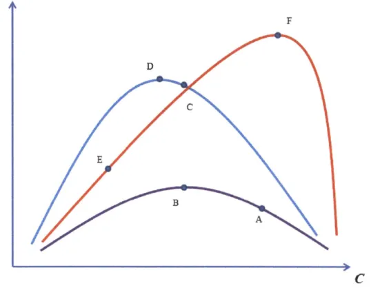
= Co, the result is the intersection of the unconstrained concave energy function with a affine linear subspace described as |Cl1 = Co , which is still a concave function. Based on this argument, we conclude that Step A2 finds the optimal solution on a concave surface. For a specific coefficient distribution C* , Step Al searches the highest energy for all different possible transform combinations T .

Graphically, the process of Algorithm A is illustrated in Figure 3-2. In this figure, we plot the energy E(T*, C) with respect to the coefficient distribution C. Each curve represents the energy function of a specific transform combination T*. Note that in practice, there are a very large number of curves and C is multi-dimensional. We simplify the figure just to show the idea.

Suppose we start from the state A and perform the iteration Step A2. Step A2 searches on the concave surface until it reaches the maximal point B. Then Step Al checks all possible transform combinations and reaches the maximal point C where

E

,

F

D

C

Figure 3-2: Graphical illustration of the iteration process of Algorithm A.

the number of coefficients used is fixed. The iteration stops when it reaches D, which

is a locally maximal solution. However, as we can see, D is different from the globally

optimal solution F, which implies that the algorithm is trapped at a local maximum.

If the algorithm starts from E and Step A2, with one step we reach the global optimum

F. We can see from this argument that the convergence may be sensitive to initial

conditions.

The best case for this algorithm is that all the locally optimal solutions are the

same. In this case, the algorithm converges to the global optimum under any initial

conditions. Even if they do not, the locally optimal solution may be very close to

the globally optimal solution. Since the structure of the energy function is dependent

on the specific signal to be evaluated, analyzing the structure in theory is difficult.

Instead, we test this property in the next chapter, by comparing the locally

opti-mal solution with the globally optiopti-mal solution obtained from the other proposed

algorithm.

In practice, there are many possible choices of initial conditions. For example, one may specify certain transforms, such as 2D-DCT for each block, and start from Step A2. One may also use an equal number of coefficients in each block and start from Step Al. The results from our simulations in the next chapter indicate that the preserved energy after convergence is not sensitive to reasonable choices of initial conditions.

3.2.4

Computational Complexity

The overall computational complexity depends on the number of iterations. In prac-tice, for typical image and video signals, the convergence occurs within several itera-tions, as shown in the next chapter. The computational complexity of one iteration can be roughly estimated as follows. We make the assumption that each transform is comparable in complexity. With the Big 0 notation which evaluates the asymptotic complexity, the computational complexity in Step Al is O(KN), when all transforms are performed and compared once in each block. For Step A2, we need to find the largest Co coefficients. This can be accomplished by sorting the coefficients with a complexity of

O(NM

log NM) , where NM equals the number of pixels. This com-plexity, however, can be improved using the median-of-medians algorithm [7], where the complexity of the worst case is O(NM) that is linear to the number of pixels. Furthermore, we note that for those blocks for which the number of coefficients chosen or the transform chosen does not change from a prior iteration, the computation can be reduced by using the results from the prior iteration. Since the majority of blocks remain to use the same transform, the intensive computations needed in computing the transforms can be drastically reduced. In conclusion, with these optimizations on the implementation of Algorithm A, it becomes a very efficient algorithm computa tionally.

3.3

Algorithm B

3.3.1

Algorithm Description

The second algorithm, denoted as Algorithm B, finds the globally optimal solution in two steps. The first step finds the optimal energy function for each block. The second step searches for the optimal solution.

In the first step, to compute the block optimal energy function, we consider a single block. For this block, when the number of coefficients used in this block is fixed, choosing the optimal transform that gives the highest energy is straightforward using the same procedure in Step Al of Algorithm A. By varying the number of coefficients used in this block, we can determine the optimal energy preserved as a function of the number of coefficients. We will refer to this function as the block optimal energy function and denote it as E(c), where c represents the number of coefficients. Note that the chosen transforms in this block optimal energy function is the only possible ones that will be selected in the optimal solution. This is because once the optimal number of coefficients used in this block is obtained in some way, the corresponding chosen transform gives the highest possible energy. As a result, it is clear that this block optimal energy function carries all the information that will be used to obtain an optimal solution.

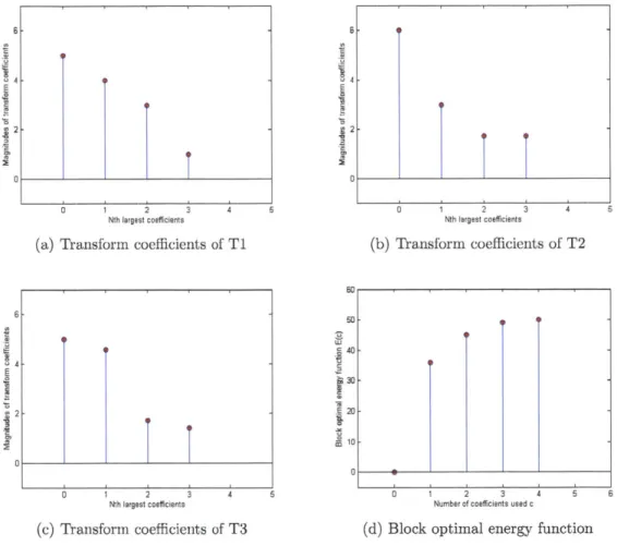
Figure 3-3 shows an example of computing the block optimal energy function. A block is transformed by three transforms T1, T2 and T3 with length four, which result

in the transform coefficients (5,4,3,1), (6,3,Vf

,v

) and

(5,v

,xf3

,v

),

shown

in Figures 3-3a, 3-3b and 3-3c respectively. To compute the block optimal energy function, we start from c = 0. For this case, we decide not using anything to preserve the energy, and the energy preservation is 0. Next, we can preserve the energy, with one coefficient, of 25,36,25 for these three transforms. Obviously, we should choose

T2 to obtain the maximal amount of energy 36. If we preserve the energy with two

coefficients, we sum up the square of the magnitudes of two largest coefficients for three transforms, which result in the energy preservation of 41,45 and 46. As a result, the optimal energy is 46 and the best transform T3 is selected. In the same manner,

when three and four coefficients are used, the optimal energy is 50 and 51, and the

best transform is T and T (or T

2

,

T

3

),

respectively. The block optimal energy

function for this specific block is given in Figure 3-3d.

2

-0

0 1 2 3 4

Nth largest coefficients (a) Transform coefficients of TI

2 04 2 0 1 2 3 4 5 LM 2

T

0 1 2 3 4 5 Nth largest coefficients (b) Transform coefficients of T2 B0 50 40 320 20 10 0 1 2 3 4 B

Nth largest coefficients Number of coefficients used c

(c) Transform coefficients of T3 (d) Block optimal energy function

Figure 3-3: An example of computing the block optimal energy function.

In the second step, we use a method to determine the optimal number of

coef-ficients used in each block. In this method, we first fix a positive parameter A and

then minimize the cost function

f(c) = c -

A

1

E(c) for each block. The parameter c

is the number of coefficients (from zero to the size of the block) and E(c) is the block

optimal energy function. The number of coefficients that leads to the minimum f(c)

is chosen as the optimal number of coefficients used in the block.

To verify that we can obtain the optimal number of coefficients used in each block

with this method, we first show that this is true for a special case when all block

optimal energy functions are concave, where A has an intuitive explanation related to the incremental energy. We then extend to the case where all block optimal energy functions are not concave.

The case when all the block optimal energy functions are concave

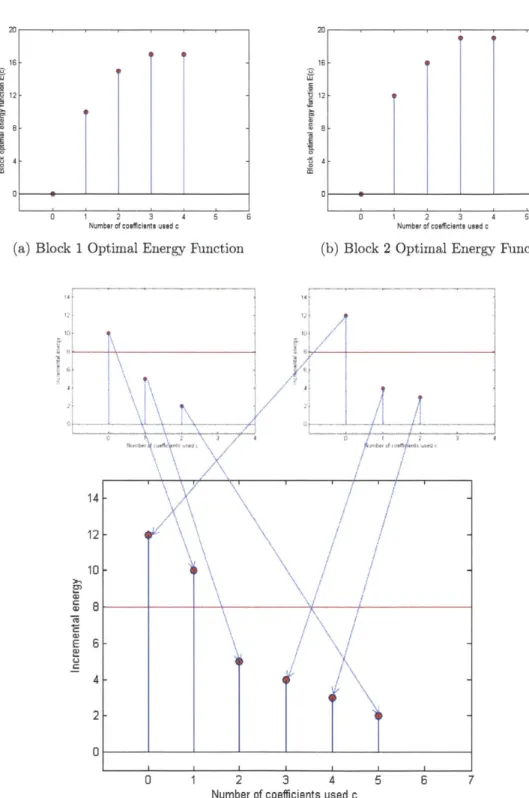
When all the block optimal energy functions are concave, we consider the incremental energy when one more coefficient is added. If the incremental energy is maximized for each new coefficient added among all the remaining coefficients in all the blocks, the cumulative energy is also maximized. This can be accomplished by computing the incremental energy from each block optimal energy function and selecting all the coefficients in all the blocks that contribute the incremental energy above a certain threshold A. All the selected coefficients can be traced back to the blocks where they come from and the optimal number of coefficients used in each block can be obtained. It will be shown that the parameter A used in the cost function f(c) represents the incremental energy threshold.

This maximization process can be illustrated with Figure 3-4. Figures 3-4a and 3-4b show optimal energy functions of two blocks. The incremental energy where one more coefficient is added in each block is shown in the left upper and right upper of Figure 3-4c. The incremental energy of all blocks can be aligned together, as is shown in the lower part of figure (c). The mapping of the incremental energy in each block to the overall incremental energy is illustrated with arrows. By decreasing the energy threshold A from 12 to 0, we can select the coefficient one by one that has the largest incremental energy in the rest of unselected coefficients. Since when all the block optimal energy functions are concave, the incremental energy is decreasing with respect to the number of coefficients used. Therefore, no smaller incremental energy will be chosen ahead of a larger one.

, 9 16 12 68 4 2 3 4 5 6

Number of coeficients used c

Optimal Energy Function

SI,

-t

0 1 2 3 4 5

Number of coeficients used c

(b) Block 2 Optimal Energy Function

0 1 2 3 4 5 6 7

Number of coefficients used c

(c) Incremental energy in each block and its mapping to the overall incremental

energy

Figure 3-4: Illustration of thresholding the incremental energy.

16 12 4 (a) L -0 1 Block 1 14 0) 0) 0) E 0) C 4

When a A is fixed, we can choose some optimal energy and the corresponding optimal numbers of coefficients used in the blocks. For example, the horizontal lines in Figure 3-4c correspond to the energy threshold A of 8. It can be seen that these two selected coefficients are distributed to both blocks using the same threshold. In this case, the optimal energy is 22 and each block will use one coefficient. This is indeed the highest amount of energy that we can preserve with two coefficients.

We now relate the process discussed above with minimizing the cost function

f

(c). Specifically, we discuss how the incremental energy thresholding can be related

with minimizing the cost function. We consider selecting all the incremental energy within a specific block that are larger than A. This can be achieved by computing the incremental energy from the block optimal energy function as E(c

+

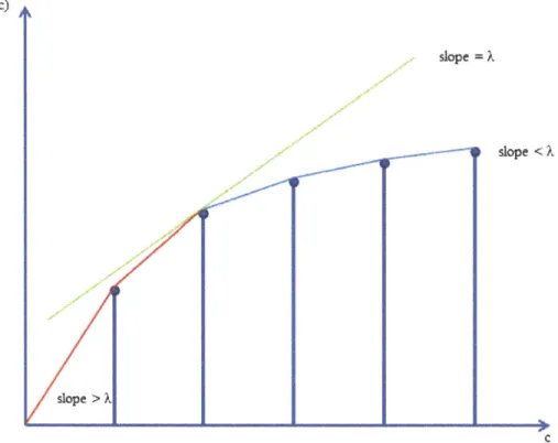
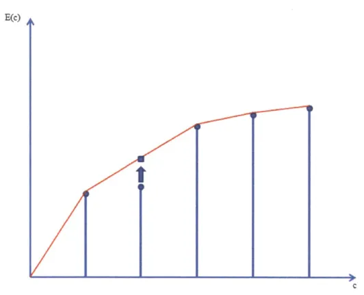
1) - E(c)

. Another approach is to directly consider E(c) . Figure 3-5 shows a concave block optimal energy function, which is linearly interpolated. It is clear that the incremental energy when a certain number of coefficients c is used is the slope of segment right to this point. In order to choose the coefficients that have incremental energy larger than A, we can instead determine the point where the slope of left segment is larger than A and that of right segment is smaller than A. This point can be determined by pushing a line with slope A until it is tangent to the interpolated function. Equivalently, pushing the line corresponds to make the intersection of the y-axis and this line as large as possible when this line is intersecting with the function. From a simple computation, we can see the intersection of this line with y axis is E(c) - Ac. Maximizing E(c) - Ac is the same as minimizing c - A-1E(c) with respect to all c. This minimizes the cost

function f (c) = c - A-'E(c) discussed above.

The case when all the block optimal energy functions are not concave

When all the block optimal energy functions are not concave, the above discussion based on the concavity of the functions case does not apply. However, every non-concave block optimal energy function can be modified to a non-concave function in the following way. We consider the convex hull of the block optimal energy function. If some values do not lie on the convex hull, we modify the values of those points to the

slope = X

-9 slope < X

C

Figure 3-5: Illustration of minimizing the cost function.

convex hull. This is illustrated in Figure 3-6. Note that this function is not concave

due to the point lying under the convex hull, which is outlined in this figure. We

modify this point straight up to the convex hull, as marked by the arrow. When all

these non-concave block optimal energy functions are modified to the concave ones,

we can apply the method discussed above to the modified problem where all the block

optimal energy functions are replaced by the concave ones.

We now show that these modifications of block optimal energy functions do not

affect the optimal solution obtained by using the minimization method discussed

above. We first observe that the values that have been modified increase due to the

property of convex hull. Intuitively, a sequence point either lies on the convex hull

or lies under the convex hull. If it lies above the convex hull, it means that the

convex hull we found is not correct. Instead, it should be modified to include the one

that lies above. This implies that the optimal energy E* we obtain in the modified

version is not smaller than that of the original E. In other words, E* is an upper

E(c)

Figure 3-6: Modification of the non-concave block optimal energy function.

bound of the optimal solution for the original problem. Another observation is that

the optimal solution obtained in the modified problem is a feasible solution in the

original problem. This can be seen from the following argument. By pushing a line

with a certain slope A, only the points that lie on the convex hull can be reached.

Therefore, those modified points will never be included into the optimal solution since

they can never be reached by the proposed method. This means the optimal numbers

of coefficients obtained will not be affected by modifying those points that lie under

the convex hull. As a result, the upper bound

E*

is actually feasible in the original

problem. We can conclude that the minimization process discussed accomplishes the

optimal number of coefficients used in each block.

We also refer to [6] for complement, since the rate-distortion optimization

dis-cussed in

[6]

has a similar mathematical structure with our method. In addition, it

provides an alternative explanation based on the Lagrangian multiplier method. The

relationship between these two explanations is quite involved. An intuitive view is

that Lagrangian multiplier method is actually derived from the duality theory, where the dual variables consider whether the optimal solution is sensitive to the infinites-imal change of some prime variables. In our explanation, we show that the optinfinites-imal solution is not sensitive to the sequence points that lie under the convex hull but is sensitive to the sequence points that lie on the convex hull.

To conclude, we outline the algorithm steps of Algorithm B:

Step B1: Compute the block optimal energy function E(c) for each block. For each block, we compute the optimal energy among the transforms within the transform set, as a function of the number of coefficients (from 0 to the size of the block M).

Step B2: Choose a fixed positive parameter A. For each block, compute f(c) =

c - A-1E(c) where c is the number of coefficients and E(c) is the block optimal energy

function. Choose the number of coefficients that minimizes f(c) as the chosen number of coefficients used in this block. Then the optimal transform for that block is the one that leads to the highest energy when the number of coefficients is given.

3.3.2

Global Optimality

As shown in the previous section, Algorithm B finds the globally optimal solution. This means for the number of coefficients used in Algorithm B, the resulting energy is the highest among all possible transform combinations and used coefficients. This global optimality is not guaranteed in Algorithm A, when the algorithm may fall into the local maximal trap. The global optimality of Algorithm B can be also be observed from the following chapter, where Algorithm B preserves higher energy relative to Algorithm A in the simulations.

3.3.3

The difficulty of specifying the total number of

coeffi-cients

The total number of coefficients used is explicitly specified in Algorithm A, while it is controlled by A in Algorithm B. The relationship between the number of coefficients used and A is complicated and cannot be determined explicitly. This brings another

issue about how to choose the correct A, which is out of the scope of this thesis. One possibility is that in order to use some specified number of coefficients, one may iterate Step B2 back and forth among different A values to match the desired number of coefficients. This method is used in this thesis. Furthermore, the possible range of A does not cover all possible total numbers of coefficients. This is because some total numbers of coefficients may be related to those points that lie under the convex hull, which can not be reached by this method. In other words, the optimal solution cannot be obtained for a certain set of total numbers of coefficients for any choice of

A.

Despite this limitation, Algorithm B is useful in verifying the convergence quality of Algorithm A. Specifically, we can specify the total number of coefficients in Algo-rithm A to exactly match that generated by a particular A in AlgoAlgo-rithm B, and see how close their solutions are. This method is used in the next chapter to evaluate the performance of Algorithm A.

3.3.4

Computational Complexity

For each block, in order to determine the block optimal energy function in Step B1, each transform needs to be performed once and compared when each number of coefficients is used. This results in O(KM) tests for one block. For all the N blocks, Step B1 has a complexity of O(NMK) . Step B2 has a complexity of O(NM) since the cost function needs to be computed M times in order to find the minimum in each block. In addition, finding the value of A that leads at least approximately to the total given number of coefficients involves performing Step B2 for multiple values of A .This fact further increases the complexity of Algorithm B.

3.4

Comparison between Two Algorithms

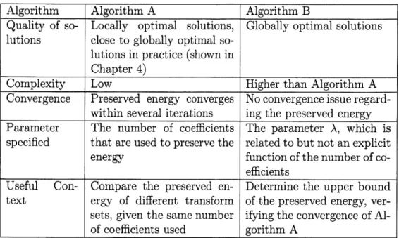
Table 3.1 summarizes the major differences between the two proposed algorithms. Algorithm A is more practical than Algorithm B mainly because of the compu-tational complexity. As analyzed in previous sections, Step Al has a complexity of

Table 3.1: Major differences between Algorithm A and Algorithm B. Algorithm Algorithm A Algorithm B

Quality of so- Locally optimal solutions, Globally optimal solutions lutions close to globally optimal

so-lutions in practice (shown in Chapter 4)

Complexity Low Higher than Algorithm A Convergence Preserved energy converges No convergence issue

regard-within several iterations ing the preserved energy Parameter The number of coefficients The parameter A, which is specified that are used to preserve the related to but not an explicit energy function of the number of

co-efficients

Useful Con- Compare the preserved en- Determine the upper bound text ergy of different transform of the preserved energy, ver-sets, given the same number ifying the convergence of Al-of coefficients used gorithm A

O(KN) and Step A2 has a complexity of O(NM), while Step B1 has a complexity

of O(MNK) and Step B2 has a complexity of O(NM). Due to the extensive

com-putation of transforms in Algorithm B relative to Algorithm A, we conclude that Algorithm B has a higher computational complexity than Algorithm A, with a factor of M, the number of data points within a block. To illustrate the idea, we consider a practical example where we use 8x8 block transforms. In this example, M is equal to 64. By using Algorithm A, the computational complexity is significantly reduced.