EpidemiOptim: a Toolbox for the Optimization of Control Policies in Epidemiological Models

HAL Id: hal-03099898

https://hal.inria.fr/hal-03099898

Preprint submitted on 6 Jan 2021

HAL is a multi-disciplinary open access

archive for the deposit and dissemination of sci-entific research documents, whether they are pub-lished or not. The documents may come from teaching and research institutions in France or abroad, or from public or private research centers.

L’archive ouverte pluridisciplinaire HAL, est destinée au dépôt et à la diffusion de documents scientifiques de niveau recherche, publiés ou non, émanant des établissements d’enseignement et de recherche français ou étrangers, des laboratoires publics ou privés.

EpidemiOptim: a Toolbox for the Optimization of

Control Policies in Epidemiological Models

Cédric Colas, Boris P. Hejblum, Sébastien Rouillon, Rodolphe Thiébaut,

Pierre-Yves Oudeyer, Clément Moulin-Frier, Mélanie Prague

To cite this version:

Cédric Colas, Boris P. Hejblum, Sébastien Rouillon, Rodolphe Thiébaut, Pierre-Yves Oudeyer, et al.. EpidemiOptim: a Toolbox for the Optimization of Control Policies in Epidemiological Models. 2020. �hal-03099898�

EpidemiOptim: a Toolbox for the Optimization of

Control Policies in Epidemiological Models

Abstract

Modelling the dynamics of epidemics helps proposing control strategies based on phar-maceutical and non-pharphar-maceutical interventions (contact limitation, lock down, vaccina-tion, etc). Hand-designing such strategies is not trivial because of the number of pos-sible interventions and the difficulty to predict long-term effects. This task can be cast as an optimization problem where state-of-the-art machine learning algorithms such as deep reinforcement learning, might bring significant value. However, the specificity of each domain – epidemic modelling or solving optimization problem – requires strong col-laborations between researchers from different fields of expertise. This is why we intro-duce EpidemiOptim, a Python toolbox that facilitates collaborations between researchers in epidemiology and optimization. EpidemiOptim turns epidemiological models and cost functions into optimization problems via a standard interface commonly used by optimiza-tion practioptimiza-tioners (OpenAI Gym). Reinforcement learning algorithms based on Q-Learning with deep neural networks (dqn) and evolutionary algorithms (nsga-ii) are already im-plemented. We illustrate the use of EpidemiOptim to find optimal policies for dynamical on-off lock-down control under the optimization of death toll and economic recess using a Susceptible-Exposed-Infectious-Removed (seir) model for COVID-19. Using EpidemiOp-tim and its interactive visualization platform in Jupyter notebooks, epidemiologists, op-timization practitioners and others (e.g. economists) can easily compare epidemiological models, costs functions and optimization algorithms to address important choices to be made by health decision-makers. Trained models can be explored by experts and non-experts via a web interface.

1. Introduction

The recent COVID-19 pandemic highlights the destructive potential of infectious diseases in our societies, especially on our health, but also on our economy. To mitigate their impact, scientific understanding of their spreading dynamics coupled with methods quantifying the impact of intervention strategies along with their associated uncertainty, are key to support and optimize informed policy making. For example, in the COVID-19 context, large scale population lock-downs were enforced based on analyses and predictions from mathematical epidemiological models (Ferguson et al., 2005, 2006; Cauchemez et al., 2019; Ferguson et al., 2020). In practice, researchers often consider a small number of relatively coarse and pre-defined intervention strategies, and run calibrated epidemiological models to predict their impact (Ferguson et al., 2020). This is a difficult problem for several reasons: 1) the space of potential strategies can be large, heterogeneous and multi-scale (Halloran et al., 2008); 2) their impact on the epidemic is often difficult to predict; 3) the problem is multi-objective by essence: it often involves public health objectives like the minimization of the death toll or the saturation of intensive care units, but also societal and economic sustainability. For these

reasons, pre-defined strategies are bound to be suboptimal. Thus, a major challenge consists in leveraging more sophisticated and adaptive approaches to identify optimal strategies.

Classically, optimal control of epidemiological model involved Pontryagin’s maximum principle or dynamic programming approaches (Pasin et al., 2018). The first approach has recently been used in the context of the COVID-19 pandemics (Lemecha Obsu & Feyissa Balcha, 2020; Perkins & Espana, 2020). However, more flexible approaches are required, especially to tackle the inherent stochasticity of the spread of infectious diseases. Hence, approaches based on reinforcement learning are emerging (Ohi et al., 2020).

Machine learning can indeed be used for the optimization of such control policies, with methods ranging from deep reinforcement learning to multi-objective evolutionary algo-rithms. In other domains, they have proven efficient at finding robust control policies, especially in high-dimensional non-stationary environments with uncertainty and partial observation of the state of the system (Deb et al., 2007; Mnih et al., 2015; Silver et al., 2017; Haarnoja et al., 2018; Kalashnikov et al., 2018; Hafner et al., 2019).

Yet, researchers in epidemiology, in public-health, in economics, and in machine learning evolve in communities that rarely cross, and often use different tools, formalizations and terminologies. We believe that tackling the major societal challenge of epidemic mitigation requires interdisciplinary collaborations organized around operational scientific tools and goals, that can be used and contributed by researchers of these various disciplines. To this end, we introduce EpidemiOptim, a Python toolbox that provides a framework to facilitate collaborations between researchers in epidemiology, economics and machine learning.

EpidemiOptim turns epidemiological models and cost functions into optimization prob-lems via the standard OpenAI Gym (Brockman et al., 2016) interface that is commonly used by optimization practitioners. Conversely, it provides epidemiologists and economists with an easy-to-use access to a variety of deep reinforcement learning and evolutionary algorithms, capable of handling different forms of multi-objective optimization under con-straints. Thus, EpidemiOptim facilitates the independent update of models by specialists of each topic, while enabling others to leverage implemented models to conduct experimental evaluations. We illustrate the use of EpidemiOptim to find optimal policies for dynamical on-off lock-down control under the optimization of death toll and economic recess using an extended Susceptible-Exposed-Infectious-Removed (seir) model for COVID-19 from Prague et al. (2020).

Related Work. We can distinguish two main lines of contributions concerning the op-timization of intervention strategies for epidemic response. On the one hand, several con-tributions focus on providing guidelines and identifying the range of methods available to solve the problem. For example, (Y´a˜nez et al., 2019) framed the problem of finding optimal intervention strategies for a disease spread as a reinforcement learning problem; (Alamo et al., 2020) provided a road-map that goes from the access to data sources to the final decision-making step; and (Shearer et al., 2020) highlighted that a decision model for epi-demic response cannot capture all of the social, political, and ethical considerations that these decisions impact. These contributions reveal a major challenge for the community: developing tools that can be easily used, configured and interpreted by decision-makers. On the other hand, computational contributions proposed actual concrete implementations

of such optimization processes. These contributions mostly differ by their definition of epidemiological models (e.g. seir (Yaesoubi et al., 2020), agent-based models (Chandak et al., 2020) or a combination of both (Kompella et al., 2020)), of optimization methods (e.g. deterministic rules (Tarrataca et al., 2020), Bayesian optimization (Chandak et al., 2020), Deep rl (Arango & Pelov, 2020; Kompella et al., 2020), optimal control (Charpen-tier et al., 2020), evolutionary optimization (Miikkulainen et al., 2020) or game-theoretic analysis (Elie et al., 2020)), of cost functions (e.g. fixed weighted sum of health and eco-nomical costs (Arango & Pelov, 2020; Kompella et al., 2020), possibly adding constraints on the school closure budget (Libin et al., 2020), or multi-objective optimization (Miikku-lainen et al., 2020)), of state and action spaces (e.g. using the entire observed epidemic history (Yaesoubi et al., 2020) or an image of the disease outbreak to capture the spatial relationships between locations (Probert et al., 2019)), as well as methods for representing the model decisions in a format suitable to decision-makers (e.g simple summary state repre-sentation (Probert et al., 2019) or real-time surveillance data with decision rules (Yaesoubi & Cohen, 2016)). See Appendix A for a detailed description of the aforementioned papers. Given this high diversity of potential methods in the field, our approach aims at pro-viding a standard toolbox facilitating the comparison of different configurations along the aforementioned dimensions in order to assist decision-makers in the evaluation of the range of possible intervention strategies.

Contributions. This paper makes three contributions. First, we formalize the coupling of epidemiological models and optimization algorithms with a particular focus on the multi-objective aspect of such problems (Section 2). Second, based on this formalization, we introduce the EpidemiOptim library, a toolbox that integrates epidemiological models, cost functions, optimization algorithms and experimental tools to easily develop, study and compare epidemic control strategies (Section 3). Third, we demonstrate the utility of the EpidemiOptim library by conducting a case study on the optimization of lock-down policies for the COVID-19 epidemic (Section 4). We use a recent epidemiological model grounded on real data, cost functions based on a standard economical model of GDP loss, as well as state-of-the-art optimization algorithms, all included in the EpidemiOptim library. This is, to our knowledge, the first contribution that provides a comparison of different optimization algorithm performances for the control of intervention strategies on the same epidemiological model. The user of the EpidemiOptim library can interact with the trained policies via a website based on Jupyter notebooks1, exploring the space of cost functions (health cost x economic cost) for a variety of algorithms. The code is made available anonymously at https://tinyurl.com/epidemioptim.

2. The Epidemic Control Problem as an Optimization Problem

In an epidemic control problem, the objective is to find an optimal control strategy to minimize some cost (e.g. health and/or economical cost) related to the evolution of an epidemic. We take the approach of reinforcement learning (rl) (Sutton & Barto, 2018): the control policy is seen as a learning agent, that interacts with an epidemiological model

1. The website will be provided in the camera-ready, as it is not anonymized. Reviewers can experience a similar interface via notebooks in the code base.

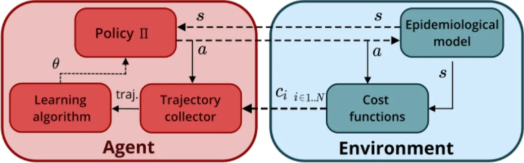
Agent Environment Epidemiological model Trajectory collector Cost functions Learning algorithm traj. Policy

Figure 1: Epidemic control as an optimization problem. s, a, ci refer to environment

states, control actions, and the ith cost, while traj. is their collection over an episode. Dashed arrows match the input and output of the OpenAI Gym step function.

that is seen as its learning environment, see Figure 1. Each run of the epidemic is a learning episode, where the agent alternatively interacts with the epidemic through actions and observes the resulting states of the environment and their associated costs. To define this optimization problem, we define three elements: 1) the state and action spaces; 2) the epidemiological model; 3) the cost function.

State and action spaces. The state st describes the information the control policy can

use (e.g. epidemiological model states, cumulative costs up to timestep t, etc.) We also need to define which actions a can be exerted on the epidemic, and how they affect its parameters. For instance, enforcing a lock-down can reduce the transmission rate of the epidemic and slow it down.

The epidemiological model. The epidemiological model is similar to a transition func-tion T : it governs the evolufunc-tion of the epidemic. From the current state st of the epidemic

and the current action atexerted by the agent, it generates the next state st+1: T : S, A → S

where S, A are the state and action spaces respectively. Note that this mapping can be stochastic.

Cost functions and constraints. The design of cost functions is central to the cre-ation of optimizcre-ation problems. Epidemic control problems can often be framed as multi-objective problems, where algorithms need to optimize for a set of cost functions instead of a unique one. Costs can be defined at the level of timesteps C(s, a) or at the level of an episode Ce(trajectory). This cumulative cost measure can be obtained by

sum-ming timestep-based costs over an episode. For mathematical convenience, rl practition-ers often use a discounted sum of costs, where future costs are discounted exponentially: Ce(trajectory) =P_tγtc(st, at) with discount factor γ (e.g. it avoids infinite sums when the

horizon is infinite). When faced with multiple cost functions Ci|i∈[1..Nc], a simple approach

is to aggregate them into a unique cost function C, computed as the convex combination of the individual costs: ¯C(s, a) = P

iβi Ci(s, a). Another approach is to optimize for the

Pareto front, i.e. the set of non-dominated solutions. A solution is said to be non-dominated if no other solution performs better on all costs and strictly better on at least one. In addi-tion, one might want to define constraints on the problem (e.g. a maximum death toll over a year).

The epidemic control problem as a Markov Decision Process. Just like traditional rl problems, our epidemic control problem can be framed as a Markov Decision Process: M : {S, A, T , ρ₀, C, γ}, where ρ0 is the distribution of initial states, see Y´a˜nez et al. (2019)

for a similar formulation.

Handling time limits. Epidemics are not episodic phenomena, or at least it is difficult to predict their end in advance. Optimization algorithms, however, require episodes of finite length. This enables the algorithm to regularly obtain fresh data by trying new policies in the environment. This can be a problem, as we do not want the control policy to act as if the end of the episode was the end of the epidemic: if the epidemic is growing rapidly right before the end, we want the control policy to care and react. Evolution algorithms (eas) cannot handle such behavior as they use episodic data (θe, Ce), where θe are the policy

parameters used for episode e. rl algorithms, however, can be made time unaware. To this end, the agent should not know the current timestep, and should not be made aware of the last timestep (termination signal). Default rl implementations often ignore this fact, see a discussion of time limits in Pardo et al. (2018).

3. The EpidemiOptim Toolbox

3.1 Toolbox Desiderata

The EpidemiOptim toolbox aims at facilitating collaborations between the different fields interested in the control of epidemics. Such a library should contain state-of-the-art epi-demiological models, optimization algorithms and relevant cost functions. It should enable optimization practitioners to bring their newly-designed optimization algorithm, to plug it to interesting environments based on advanced models grounded in epidemiological knowl-edge and data, and to reliably compare it to other state-of-the-art optimization algorithms. On the other hand, it should allow epidemiologists to bring their new epidemiological model, reuse existing cost functions to form a complete epidemic control problem and use state-of-the-art optimization algorithms to solve it. This requires a modular approach where algorithms, epidemiological models and cost functions are implemented independently with a standardized interface. The toolbox should contain additional tools to facilitate experi-ment manageexperi-ment (result tracking, configuration saving, logging). Good visualization tools would also help the interpretation of results, especially in the context of multi-objective problems. Ideally, users should be able to interact with the trained policies, and to ob-serve the new optimal strategy after the modification of the relative importance of costs in real-time. Last, the toolbox should enable reproducibility (seed management) and facilitate statistical comparisons of results.

3.2 Toolbox Organization

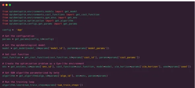
Overview. The EpidemiOptim toolbox is centered around two modules: the environment and the optimization algorithm, see Figure 1. To run an experiment, the user can define its own or select the ones contained in the library. Figure 2 presents the main interface of the EpidemiOptim library. The following sections delve into the environment and algorithm modules.

Figure 2: Main running script of the EpidemiOptim library

Environment: epidemiological models. The Model module wraps around epidemio-logical models, and allows to sample new model parameters from a distribution of models, to sample initial conditions (ρ0) and to run the model for n steps. Currently, the

Epi-demiOptim library contains a Python implementation of an extended Susceptible-Exposed-Infectious-Removed (seir) model fitted to French data, from Prague et al. (2020).

Environment: cost functions and constraints. In the EpidemiOptim toolbox, each cost function is a separate class that can compute ci(s, a), normalize the cost to [0, 1] and

generate constraints on its cumulative value. The Multi-Cost module integrates several cost functions. It computes the list of costs ci(s, a)|i∈[1..Nc] and an aggregated cost ¯c

parame-terized by the mixing weights βi|i∈[1..Nc]. The current version of EpidemiOptim contains

two costs: 1) a health cost computed as the death toll of the epidemic; 2) an economic cost computed as the opportunity loss of GDP resulting from either the epidemic itself (ill-ness and death reduce the workforce), or the control strategies (lock-down also reduces the workforce). We define two additional parameterized constraints. For each of the costs, the cumulative value should stay below a threshold. This threshold can vary and is controlled by the agent. For each episode, the agent selects constraints (thresholds) on the two costs and behaves accordingly.

Environment: OpenAI Gym interface as a universal interface. The learning envi-ronment defines the optimization problem. We use a framework that has become standard in the Reinforcement Learning community in recent years: the OpenAI Gym environment (Brockman et al., 2016). Gym environments have the following interface: First, they have a reset function that resets the environment state, effectively starting a new simulation or episode. Second, they have a step function that takes as input the next action from the control policy, updates the internal state of the model and returns the new environment state, the cost associated to the transition and a Boolean signal indicating whether the episode is terminated, see Figure 1. This standardized interface allows optimization

practi-tioners (rl researchers especially) to easily plug any algorithm, facilitating the comparison of algorithms on diverse benchmark environments. In our library, this class wraps around an epidemiological model and a set of cost functions. It also defines the state and action spaces S, A. So far, it contains the EpidemicDiscrete-v0 environment, a Gym-like envi-ronment based on the epidemiological model and the bi-objective cost function described above. Agents decide every week whether to enforce a partial lock-down (binary action) that results in a decreased transmission rate. Note that the step size (here one week) can easily be modified.

Optimization algorithms. The optimization algorithm, or algorithm for short, trains learning agents to minimize cumulative functions of costs. Learning agents are characterized by their control policy: a function that takes the current state of the environment as input and produces the next action to perform: Πθ : S → A where Πθ is parameterized by the

vector θ. The objective of the algorithm is, thus, to find the optimal set of parameters θ∗ that minimizes the cost. These algorithms collect data by letting the learning agent interact with the environment. Currently, the EpidemiOptim toolbox integrates several rl algorithms based on the famous Deep Q-Network algorithm (Mnih et al., 2015) as well as the state-of-the-art multi-objective ea nsga-ii (Deb et al., 2002).

Utils. We provide additional tools for experimentation: experience management, logging and plots. Algorithms trained on the same environment can be easily compared, e.g. by plotting their Pareto front on the same graph. We also enable users to visualize and interact with trained policies via Jupyter notebooks or a web interface accessible to non-experts. Users can select solutions from the Pareto front, modify the balance between different cost functions and modify the value of constraints set to the agent via sliders. They visualize a run of the resulting policy in real-time. We are also committed to reproducibility and robustness of the results. For this reason, we integrate to our framework a library for statistical comparisons designed for rl experiments (Colas et al., 2019).

4. Case Study: Lock-Down On-Off Policy Optimization for the COVID-19 Epidemic

The SARS-CoV-2 virus was identified on January, 7th 2020 as the cause of a new viral disease named COVID-19. As it rapidly spread globally, the World Health Organization (2020) declared a pandemic on March 11th 2020. Exceptional measures have been imple-mented across the globe as an attempt to mitigate the pandemic (Kraemer et al., 2020). In many countries, the government response was a total lock-down: self-isolation with so-cial distancing, schools and workplaces closures, cancellation of public events, large and small gatherings prohibition, and travel limitation. In France, first lock-down lasted 55 days from March, 17th to May, 11th. It led to a decrease in gross domestic product of, at least, 10.1% (Mandel & Veetil, 2020) but allowed to reduce the death toll by an estimated 690,000 [570,000; 820,000] people (Flaxman et al., 2020). A second lock-down lasted from October, 30th to December, 15th, illustrating that on-off lock-down strategies seem to be a realistic policy in population with low herd immunity and in absence, or with low coverage, of vaccine. In this case study, we investigate alternative strategies optimized by rl and ea algorithms over a period of 1 year.

4.1 Environment

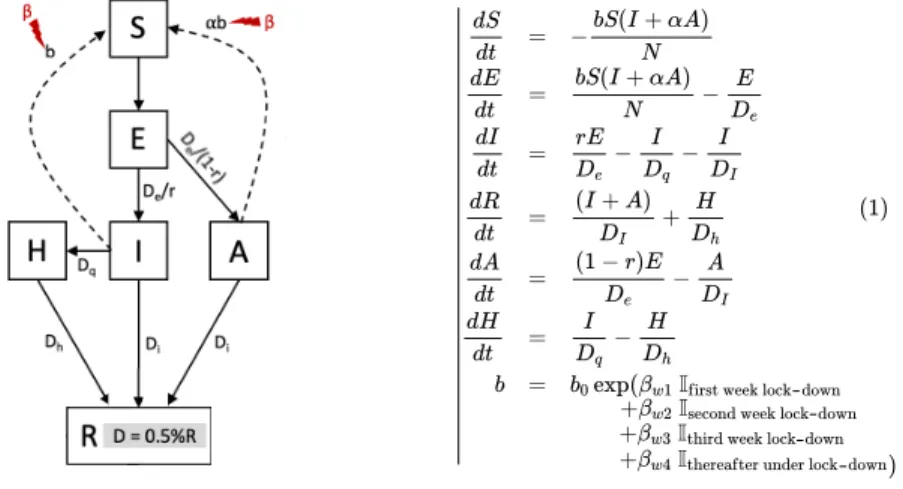
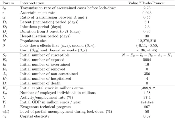
The epidemiological model. We use a mathematical structural model to understand the large-scale dynamics of the COVID-19 epidemic. We focus on the extended Susceptible-Exposed-Infectious-Removed (seir) model from Prague et al. (2020), which was fitted to French data. The estimation in this model was region-specific. Here, we use their estimated parameters for the epidemic dynamics in ˆIle-de-France (Paris and its surrounding region), see parameters description and mean values in Table 1. The model explains the dynamics between Susceptibles (S), Exposed (E), Ascertained Infectious (I), Removed (R), Non-Ascertained Infectious (A) and Hospitalized (H). The underlying system of differential equations (1) and a schematic view of the mechanistic model can be found in Figure 3. The transmission rate b is modified each week after lock-down with a step function: it decreases from week 1 to week 4 after lock-down and then remains constant for any following week under lock-down. To account for uncertainty in the model parameters, we create a distribution of models resulting from parameter distributions, see details in Appendix Section B and a visualization of 10 sampled models in Appendix Section B.2.

Figure 3: Description of the seirah epidemiological model. Schematic and system of dif-ferential equations. Susceptible individuals S can be infected by ascertained (I) and non-ascertained (A) infectious individuals by a law mass action depending on the transmission rate β and αβ (reduced transmission for non-ascertained infectious). Once Exposed E, in-dividuals take in average De days to become infectious, among which r are non-ascertained

(possibly because they are asymptomatic or pauci-symptomatic or simply not tested for COVID-19). Only ascertained infectious individual can proceed to hospitalization (H) at rate Dq. After in average Di and Dh days, infectious and hospitalized individuals recover

(R). We assume that 0.5% of recovered are dead (D). Transmission rate is modelled with a step function modeling week after week the decrease in transmission after lock-down. Lock-down effect takes 4 weeks to establish. See Prague et al. (2020) for more details and rational.

State and action spaces. The state of the agent is composed of the epidemiological states (seirah) normalized by the population size (N = 12, 278, 210), booleans indicating

Param. Interpretation Value ”Ile-de-France” b0 Transmission rate of ascertained cases before lock-down 2.23

r Ascertainement rate 0.043

α Ratio of transmission between A and I 0.55

De Latent (incubation) period (days) 5.1

DI Infectious period (days) 2.3

Dq Duration from I onset to H (days) 0.36

Dh Hospitalization period (days) 30

N Population size 12,278,210

β Lock-down effects first (βw1), second (βw2), (-0.11, -0.50,

third (βw3) and thereafter weeks (βw0) -1.36, -1.46)

S0 Initial number of susceptible N − E0− I0− R0− A0− H0

E0 Initial number of exposed 5004

I0 Initial number of ascertained 16

R0 Initial number of removed 0

A0 Initial number of non ascertained 356

H0 Initial number of hospitalized 4

D0 Initial number of death 0

K0 Initial capital stock in millions euros 1,388,912

L0 Number of employed individuals in millions 4.58

λ Activity/employment rate (%) 37.4

Y0 Initial GDP in million euros / year 424,474

A Exogenous technical progress 867

u(t) Level of partial unemployment during lock-down (%) 50

γk Capital elasticity 0.37

Table 1: Parameter values for the ˆIle-de-France region for the seirah epidemiological model and the economy cost function.

whether the previous and current state are under lock-down, the two cumulative costs and the level of the transmission rate (from week 1 to week 4 and after). As described in previous section, consecutive weeks of lockdown decrease the transmission b in four stages, while stopping lockdown follows the opposite path (stair-case increase of b). The two cumulative costs are normalized by N and 150 billion euros (B€); respectively, 150 B€ being the approximate maximal cost due to a full year of lockdown. The action occurs weekly and is binary (1 for lock-down, 0 otherwise).

Cost functions. In this case-study, an optimal policy should minimize two costs: a health cost and an economic cost. The health cost is computed as the death toll, it can be evaluated for each environment transition (weekly) or over a full-episode (e.g. annually): Ch(t) = D(t) = 0.005R(t).

The economic cost is measured in euros as the GDP opportunity cost resulting from dis-eased or dead workers, as well as people unemployed due to the lock-down policy. At any time t, the GDP can be expressed as a Cobb-Douglas function F (L(t)) = AK₀γkL(t)1−γk, where K0 is the capital stock of economy before the outbreak that we will suppose constant

during the pandemics, L(t) is the active population employed, γkis the capital elasticity and

A is the exogenous technical progress (Douglas, 1976). Let L0 = λN be the initial employed

population, where λ is the activity/employment rate. The lock-down leads to partial un-employment and decreases the size of the population able to work (illness, isolation, death), thus L(t) = (1 − u(t))λ(N − G(t)), where u(t) is the level of partial unemployment due to the lock-down and G(t) = I(t) + H(t) + 0.005R(t) is the size of the ill, isolated or dead population as defined in our seirah model. The economic cost is defined as the difference between the GDP before (Y0) and after the pandemic, Y0− F (L(t)) and is given by:

Ceco(t) = Y0− AK0γk((1 − u(t))λ(N − G(t)) 1−γk

Parameters for values of parameters in the economic model are given in Table 1 and are derived from the National Institute of Statistics and Economical Analysis (Insee, 2020) and (Havik et al., 2014). We also consider the use of constraints on the maximum value of cumulative costs.

4.2 Optimization Algorithms

We consider three algorithms: 1) a vanilla implementation of Deep Q-Network (dqn) (Mnih et al., 2015); 2) a goal-conditioned version of dqn inspired from (Schaul et al., 2015); 3) nsga-ii, a state-of-the-art multi-objective evolutionary algorithm (Deb et al., 2002). The trained policy is the same for all algorithms: a neural network with one hidden-layer of size 64 and ReLU activations. Further background about these algorithm is provided in Appendix Section B.

Optimizing convex combinations of costs: DQN and Goal DQN. dqn only targets one cost function: ¯c = (1−β) ch+β ceco. Here the health and economic costs are normalized

to have similar ranges (scaled by 1/(65×1e3) and 1/1e9 respectively). We train independent policies for each values of β in [0., 0.05, .., 1]. This consists in training a Q-network to estimate the value of performing any given action a in any given state s, where the value is defined as the cumulative negative cost −¯c expected in the future. goal dqn, however,

trains one policy Π(s, β) to target any convex combination parameterized by β. We use the method presented in (Badia et al., 2020): we train two Q-networks, one for each of the two costs. The optimal action is then selected as the one maximizing the convex combination of the two Q-values:

Π(s, β) = argmax_a(1 − β) Qs(s, a) + β Qeco(s, a). (1)

By disentangling the two costs, this method facilitates the representation of values that can have different scales and enables automatic transfer for any value of β, see justifications in Badia et al. (2020). During training, agents sample the targeted β uniformly in [0, 1]. Adding constraints with Goal DQN-C. We design and train a variant of goal dqn to handle constraints on maximal values for the cumulative costs: goal dqn-c. We train a Q-network for each constraints with a cost of 1 each time the constraint is violated, 0 otherwise (Qc_h, Qc_eco). With a discount factor γ = 1, this network estimates the number of transitions that are expected to violate the constraints in the future. The action is selected according to Eq. 1 among the actions that are not expected to lead to constraints violations (Qc(s, a) < 1). If all actions are expected to lead to violations, the agent selects the action that minimizes that violation. During training, agents sample β uniformly, and 50% of the time samples uniformly one of the two constraints in [1000, 62000] for the maximum death toll and [20, 160] for the maximum economic cost, in billions.

EAs to optimize a Pareto front of solutions. We also use nsga-ii, a state-of-the-art multi-objective ea algorithm that trains a population of solutions to optimize a Pareto front of non-dominated solutions (Deb et al., 2002). As others eas, nsga-ii uses episodic data (θe, Ce). To obtain reliable measures of Ce in our stochastic environment, we average

costs over 30 evaluations. For this reason, nsga-ii requires more samples than traditional gradient-based algorithms. For fair comparison, we train two nsga-ii algorithm: one with the same budget of samples than dqn variants (1e6 environment steps), and the other with 15x as much (after convergence).

4.3 Results

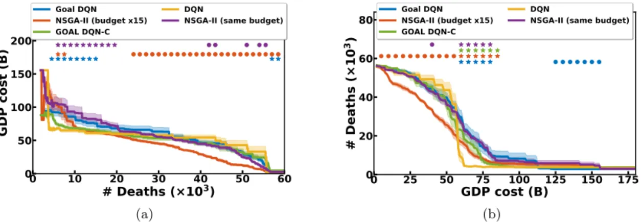
Pareto fronts. We aim at providing decision tools to decision-maker and, for this reason, cannot decide ourselves the right value for the mixing parameter β. Instead, we want to present Pareto fronts of Pareto-optimal solutions. Only nsga-ii aims at producing an optimal Pareto front as its result while dqn and goal dqn optimize a unique policy. However, one can build Pareto fronts even with dqn variants. We can build population of policies by aggregating independently trained dqn policies, or evaluating a single goal dqn policy on a set of Npareto goals sampled uniformly (100 here). The resulting population

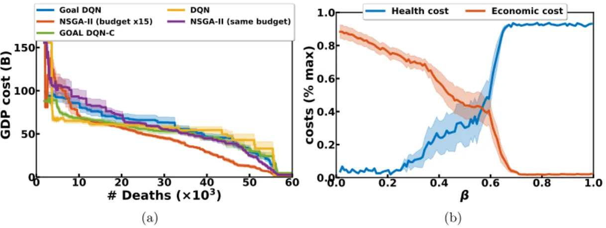
can then be filtered to produce the Pareto front. Figure 4a presents the resulting Pareto fronts for all variants. The Pareto fronts made of several dqn policies (yellow) perform better in the regime of low health cost (< 103 deaths) where it leads to save around 20 billion euros over nsga-ii and the goal dqn without constraint. Over 25 × 103 deaths, nsga-ii becomes the best algorithm, as it allows to save 10 to 15 billion euros in average, the health cost being kept constant. Note that using more objectives might require other visualization tools (see discussion in He and Yen (2015), Ishibuchi et al. (2008)). Running

times are about 2 hours for dqn, 4 hours for goal dqn and 10 hours for nsga-ii on a single cpu. 0 10 20 30 40 50 60 # Deaths (×103₎ 0 50 100 150 GDP cost (B) Goal DQN NSGA-II (budget x15) GOAL DQN-C DQN

NSGA-II (same budget)

(a) 0.0 0.2 0.4 0.6 0.8 1.0 β 0.0 0.2 0.4 0.6 0.8 1.0 costs (% max)

Health cost Economic cost

(b)

Figure 4: Left: Pareto fronts for various optimization algorithms. The closer to the origin point the better. Right: Evolution of the costs when goal dqn agents are evaluated on various β. We plot the mean and standard error of the mean (left) and standard deviations (right) over 10 seeds.

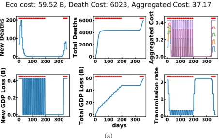
In the low health cost regime, the dqn policy attempts to break the first wave of the epidemic, then maintains it low with periodic lock-down (1 or 2 weeks period) until it is sufficiently low. If a second wave appears, it goes back to that strategy, see Figure 5a for an example. goal dqn with constraints shows a similar behavior. nsga-ii enters a cyclic 1-week period of lock-down but does not stop it even when the number of new cases appears null (Appendix Section C). In the low economic cost regime (below 15 B€), nsga-ii waits for the first wave to grow and breaks it by a lock-down of a few weeks (Figure 5b). dqn-based algorithms sometimes find such policies. Policies in the range of health cost between 103 and 50 × 103 deaths are usually policy that perform low or high health costs depending on the particular epidemic and its initial state. Appendix Section 4.3 presents comparison statistics and delves into the different strategies and interesting aspects of the four algorithms.

Optimizing convex combinations. When β is low (respectively high), the cost function is closer to the health (respectively economic) cost (see Eq 1). Figure 4b presents the evolution of the two costs when a trained goal dqn policy (without constraints) is evaluated on different β. As expected, the higher β the lower the health cost and vice-versa. We see that, outside of the [0.2, 0.8] range, the policy falls in extreme regimes: either it always locks-down (low β) or it never does (high β).

Interactive decision making. The graphs presented above help make sense of the gen-eral performance of the algorithms, in average over multiple runs. However, it is also relevant to look at particular examples to understand a phenomenon. For this purpose, we include visualization Jupyter Notebooks in the EpidemiOptim toolbox. There are three notebooks for dqn, goal dqns and nsga-ii respectively. The two first one help making sense of dqn and goal dqn algorithms (with or without constraints). After loading a pre-trained

model, the user can interactively act on the cost function parameters (mixing weight β or constraints on the maximum values of the cumulative costs). As the cost function changes, the policy automatically adapts and the evolution of the epidemic and control strategy are displayed. The third notebook helps visualizing a Pareto front of the nsga-ii algorithm. After loading a pre-trained model, the user can click on solutions shown on the Pareto front, which automatically runs the corresponding model and displays the evolution of the epi-demic and control strategy. The user can explore these spaces and visualize the strategies that correspond to the different regimes of the algorithm. We also wrap these notebooks in a web interface accessible to non-experts. In addition to running trained models, users can also attempt to design their own lockdown policy within the web interface and compare their performance to the one of trained models on the Pareto front.

0 100 200 300 0 100 200

New Deaths

Total Deaths

Aggregated Cost

New GDP Loss (B)

days

Total GDP Loss (B)

Transmission rate

Eco cost: 59.52 B, Death Cost: 6023, Aggregated Cost: 37.17

(a) 0 100 200 300 0 1000

New Deaths

Total Deaths

Aggregated Cost

New GDP Loss (B)

_days

Total GDP Loss (B)

Transmission rate

Eco cost: 13.09 B, Death Cost: 41216, Aggregated Cost: 38.25

(b)

Figure 5: Evolution of cost metrics and strategy over a year of simulated epidemic with a dqn agent (top) in the low health cost regime and a nsga-ii agent in the low economic cost regime (bottom).

Discussion. This case study proposed to use a set of state-of-the-art algorithms to target the problem of lock-down policy optimization in the context of the COVID-19 epidemic (rl and ea algorithms). dqn appears to work better in the regime of low health cost, but requires to train multiple policies independently. As it trains only one policy, goal dqn is faster, but does not bring any performance advantage. nsga-ii, which is designed for the purpose of multi-objective optimization, seems to perform better in the regime of low economic cost. Overall, we see emerging two different strategies: one with either a single early lockdown or none at all that seems to rely on herd immunity and one that systematically enforces short-term lockdowns to control the evolution of the epidemic and avoid important epidemic waves. In the last months, few countries have pursued the ”herd immunity” strategy and its efficacy is still being questioned (e.g. in Sweden Orlowski and Goldsmith (2020)). On the other hand, most of the countries that were strongly affected went for the second strategy: enforcing lockdown when the number of cases rises, to contain the epidemic waves. In practice, lockdown is often enforced for at least a month – probably due to political and practical reasons – which contrasts with the shorter lockdowns (one or two weeks) often used by our control policies.

5. Discussion & Conclusion

On the use of automatic optimization for decision-making. We do not think that optimization algorithms should ever replace decision-makers, especially in contexts involv-ing the life and death of individuals such as epidemics. However, we think optimization algorithms can provide decision-makers with useful insights by taking into account long-term effects of control policies. To this end, we believe it is important to consider a wide range of models and optimization algorithms to target a same control problem. This fosters a diversity of methods and reduces the negative impacts of model- and algorithm-induced biases. The EpidemiOptim toolbox is designed for this purpose: it provides a one-stop shop centralizing both the modeling and the optimization in one place.

The future of EpidemiOptim. This toolbox is designed as a collaborative toolbox that will be extended in the future. To this day, it contains one population-based seir epidemi-ological models and three optimization algorithms. In the future, we plan on extending this library via collaborations with other research labs in epidemiology and machine learning. We plan on integrating agent-based epidemiological models that would allow a broader range of action modalities, and to add a variety of multi-objective algorithms from eas and rl. We could finally imagine the organization of challenges, where optimization practitioners would compete on a set of epidemic control environments.

Although this toolbox focuses on the use of optimization algorithm to solve epidemic control policies, similar tools could be used in other domains. Indeed, just like epidemics, a large diversity of dynamical systems can be modeled models by ordinary differential equations (e.g. in chemistry, biology, economics, etc.). One could imagine spin-offs of EpidemiOptim for applications to other domains. Furthermore, Chen et al. (2018) recently designed a differentiable ODE solver. Such solvers could be integrated to EpidemiOptim to allow differential learning through the model itself.

Conclusion. This paper introduces EpidemiOptim, a toolbox that facilitates collabora-tion between epidemiologists, optimizacollabora-tion practicollabora-tioners and others in the study of epidemic control policies to help decision-making. Of course, others have studied the use of optimiza-tion algorithms for the control of epidemics. We see this as a strength, as it shows the relevance of the approach and the importance of centralizing this research in a common framework that allows easy and reproducible comparisons and visualizations. Articulat-ing our understandArticulat-ing of epidemics evolution with the societal impacts of potential control strategies on the population (death toll, physical and psychological traumas, etc) and on the economy will help improve the control of future epidemics.

Acknowledgments

References

Alamo, T., Reina, D. G., & Mill´an, P. (2020). Data-Driven Methods to Monitor, Model, Forecast and Control Covid-19 Pandemic: Leveraging Data Science, Epidemiology and Control Theory. arXiv preprint arXiv:2006.01731.

Arango, M., & Pelov, L. (2020). COVID-19 Pandemic Cyclic Lockdown Optimization Using Reinforcement Learning. arXiv preprint arXiv:2009.04647.

Badia, A. P., Piot, B., Kapturowski, S., Sprechmann, P., Vitvitskyi, A., Guo, D., & Blundell, C. (2020). Agent57: Outperforming the atari human benchmark. arXiv preprint arXiv:2003.13350.

Brockman, G., Cheung, V., Pettersson, L., Schneider, J., Schulman, J., Tang, J., & Zaremba, W. (2016). Openai gym. arXiv preprint arXiv:1606.01540.

Cauchemez, S., Hoze, N., Cousien, A., Nikolay, B., et al. (2019). How modelling can enhance the analysis of imperfect epidemic data. Trends in parasitology, 35 (5), 369–379. Chandak, A., Dey, D., Mukhoty, B., & Kar, P. (2020). Epidemiologically and

socio-economically optimal policies via bayesian optimization. arXiv preprint arXiv:2005.11257.

Charpentier, A., Elie, R., Lauri`ere, M., & Tran, V. C. (2020). COVID-19 pandemic control: balancing detection policy and lockdown intervention under ICU sustainability.. Chen, R. T., Rubanova, Y., Bettencourt, J., & Duvenaud, D. K. (2018). Neural ordinary

differential equations. In Advances in neural information processing systems, pp. 6571–6583.

Colas, C., Sigaud, O., & Oudeyer, P.-Y. (2019). A Hitchhiker’s Guide to Statistical Com-parisons of Reinforcement Learning Algorithms. arXiv preprint arXiv:1904.06979. Deb, K., Karthik, S., et al. (2007). Dynamic multi-objective optimization and

decision-making using modified NSGA-II: a case study on hydro-thermal power scheduling. In International conference on evolutionary multi-criterion optimization, pp. 803–817. Springer.

Deb, K., Pratap, A., Agarwal, S., & Meyarivan, T. (2002). A fast and elitist multiobjective genetic algorithm: NSGA-II. IEEE transactions on evolutionary computation, 6 (2), 182–197.

Douglas, P. H. (1976). The Cobb-Douglas Production Function Once Again: Its History, Its Testing, and Some New Empirical Values. Journal of Political Economy, 84 (5), 903–915.

Elie, R., Hubert, E., & Turinici, G. (2020). Contact rate epidemic control of COVID-19: an equilibrium view. Mathematical Modelling of Natural Phenomena, 15, 35.

Ferguson, N., Laydon, D., Nedjati Gilani, G., Imai, N., Ainslie, K., Baguelin, M., Bhatia, S., Boonyasiri, A., Cucunuba Perez, Z., Cuomo-Dannenburg, G., et al. (2020). Report 9: Impact of non-pharmaceutical interventions (NPIs) to reduce COVID19 mortality and healthcare demand..

Ferguson, N. M., Cummings, D. A., Cauchemez, S., Fraser, C., Riley, S., Meeyai, A., Iamsirithaworn, S., & Burke, D. S. (2005). Strategies for containing an emerging influenza pandemic in Southeast Asia. Nature, 437 (7056), 209–214.

Ferguson, N. M., Cummings, D. A., Fraser, C., Cajka, J. C., Cooley, P. C., & Burke, D. S. (2006). Strategies for mitigating an influenza pandemic. Nature, 442 (7101), 448–452. Flaxman, S., Mishra, S., Gandy, A., Unwin, H. J. T., Mellan, T. A., Coupland, H., Whit-taker, C., Zhu, H., Berah, T., Eaton, J. W., et al. (2020). Estimating the effects of non-pharmaceutical interventions on COVID-19 in Europe. Nature, 584 (7820), 257–261.

Haarnoja, T., Zhou, A., Abbeel, P., & Levine, S. (2018). Soft actor-critic: Off-policy maximum entropy deep reinforcement learning with a stochastic actor. In Proceedings of ICML.

Hafner, D., Lillicrap, T., Ba, J., & Norouzi, M. (2019). Dream to control: Learning behav-iors by latent imagination. In Proceedings of ICLR.

Halloran, M. E., Ferguson, N. M., Eubank, S., Longini, I. M., Cummings, D. A., Lewis, B., Xu, S., Fraser, C., Vullikanti, A., Germann, T. C., et al. (2008). Modeling targeted layered containment of an influenza pandemic in the United States. Proceedings of the National Academy of Sciences, 105 (12), 4639–4644.

Havik, K., Mc Morrow, K., Orlandi, F., Planas, C., Raciborski, R., R¨oger, W., Rossi, A., Thum-Thysen, A., Vandermeulen, V., et al. (2014). The production function method-ology for calculating potential growth rates & output gaps. Tech. rep., Directorate General Economic and Financial Affairs (DG ECFIN), European . . . .

He, Z., & Yen, G. G. (2015). Visualization and performance metric in many-objective optimization. IEEE Transactions on Evolutionary Computation, 20 (3), 386–402. Insee (2020). Insee Website. https://www.insee.fr/.

Ishibuchi, H., Tsukamoto, N., & Nojima, Y. (2008). Evolutionary many-objective optimiza-tion: A short review. In 2008 IEEE Congress on Evolutionary Computation (IEEE World Congress on Computational Intelligence), pp. 2419–2426. IEEE.

Kalashnikov, D., Irpan, A., Pastor, P., Ibarz, J., Herzog, A., Jang, E., Quillen, D., Holly, E., Kalakrishnan, M., Vanhoucke, V., et al. (2018). Scalable deep reinforcement learning for vision-based robotic manipulation. In Conference on Robot Learning, pp. 651–673. Kompella, V., Capobianco, R., Jong, S., Browne, J., Fox, S., Meyers, L., Wurman, P., & Stone, P. (2020). Reinforcement Learning for Optimization of COVID-19 Mitigation policies..

Kraemer, M. U. G., Yang, C.-H., Gutierrez, B., Wu, C.-H., Klein, B., Pigott, D. M., du Plessis, L., Faria, N. R., Li, R., Hanage, W. P., Brownstein, J. S., Layan, M., Vespignani, A., Tian, H., Dye, C., Pybus, O. G., & Scarpino, S. V. (2020). The effect of human mobility and control measures on the COVID-19 epidemic in China. Science, 368 (6490), 493–497.

Lemecha Obsu, L., & Feyissa Balcha, S. (2020). Optimal control strategies for the trans-mission risk of COVID-19. Journal of biological dynamics, 14 (1), 590–607.

Libin, P., Moonens, A., Verstraeten, T., Perez-Sanjines, F., Hens, N., Lemey, P., & Now´e, A. (2020). Deep reinforcement learning for large-scale epidemic control. arXiv preprint arXiv:2003.13676.

Mandel, A., & Veetil, V. P. (2020). The Economic Cost of COVID Lockdowns: An Out-of-Equilibrium Analysis. Economics of Disasters and Climate Change.

Miikkulainen, R., Francon, O., Meyerson, E., Qiu, X., Canzani, E., & Hodjat, B. (2020). From Prediction to Prescription: AI-Based Optimization of Non-Pharmaceutical In-terventions for the COVID-19 Pandemic. arXiv preprint arXiv:2005.13766.

Mnih, V., Kavukcuoglu, K., Silver, D., Rusu, A. A., Veness, J., Bellemare, M. G., Graves, A., Riedmiller, M., Fidjeland, A. K., Ostrovski, G., et al. (2015). Human-level control through deep reinforcement learning. nature, 518 (7540), 529–533.

Ohi, A. Q., Mridha, M., Monowar, M. M., & Hamid, M. A. (2020). Exploring optimal control of epidemic spread using reinforcement learning. Scientific Reports, 10. Orlowski, E. J., & Goldsmith, D. J. (2020). Four months into the COVID-19 pandemic,

Sweden’s prized herd immunity is nowhere in sight. Journal of the Royal Society of Medicine, 113 (8), 292–298.

Pardo, F., Tavakoli, A., Levdik, V., & Kormushev, P. (2018). Time limits in reinforcement learning. In International Conference on Machine Learning, pp. 4045–4054.

Pasin, C., Dufour, F., Villain, L., Zhang, H., & Thi´ebaut, R. (2018). Controlling IL-7 injections in HIV-infected patients. Bulletin of mathematical biology, 80 (9), 2349– 2377.

Perkins, A., & Espana, G. (2020). Optimal control of the COVID-19 pandemic with non-pharmaceutical interventions. medRxiv.

Prague, M., Wittkop, L., Clairon, Q., Dutartre, D., Thi´ebaut, R., & Hejblum, B. P. (2020). Population modeling of early COVID-19 epidemic dynamics in French regions and estimation of the lockdown impact on infection rate. medRxiv.

Probert, W. J. M., Lakkur, S., Fonnesbeck, C. J., Shea, K., Runge, M. C., Tildesley, M. J., & Ferrari, M. J. (2019). Context matters: using reinforcement learning to develop human-readable, state-dependent outbreak response policies. Philosophical Transactions of the Royal Society B: Biological Sciences, 374 (1776), 20180277.

Schaul, T., Horgan, D., Gregor, K., & Silver, D. (2015). Universal value function approxi-mators. In International conference on machine learning, pp. 1312–1320.

Shearer, F. M., Moss, R., McVernon, J., Ross, J. V., & McCaw, J. M. (2020). Infec-tious disease pandemic planning and response: Incorporating decision analysis. PLoS medicine, 17 (1), e1003018.

Silver, D., Schrittwieser, J., Simonyan, K., Antonoglou, I., Huang, A., Guez, A., Hubert, T., Baker, L., Lai, M., Bolton, A., et al. (2017). Mastering the game of go without human knowledge. nature, 550 (7676), 354–359.

Sutton, R. S., & Barto, A. G. (2018). Reinforcement learning: An introduction. MIT press. Tarrataca, L., Dias, C., Haddad, D. B., & Arruda, E. (2020). Flattening the curves: on-off lock-down strategies for COVID-19 with an application to Brazil. arXiv preprint arXiv:2004.06916.

Watkins, C. J., & Dayan, P. (1992). Q-learning. Machine learning, 8 (3-4), 279–292. World Health Organization (2020). WHO Director-General’s opening remarks at the media

briefing on COVID-19 – 11 March 2020.. Accessed: 2020-04-02.

Yaesoubi, R., & Cohen, T. (2016). Identifying cost-effective dynamic policies to control epidemics. Statistics in medicine, 35 (28), 5189–5209.

Yaesoubi, R., Havumaki, J., Chitwood, M. H., Menzies, N. A., Gonsalves, G., Salomon, J., Paltiel, A. D., & Cohen, T. (2020). Adaptive policies for use of physical distancing interventions during the COVID-19 pandemic. medRxiv.

Y´a˜nez, A., Hayes, C., & Glavin, F. (2019). Towards the Control of Epidemic Spread: Designing Reinforcement Learning Environments.. In AICS, pp. 188–199.

Appendix A. Additional Related Work

Prior to the current COVID-19 pandemics, Y´a˜nez et al. (2019) framed the problem of find-ing optimal intervention strategies for a disease spread as a reinforcement learnfind-ing problem, focusing on how to design environments in terms of disease model, intervention strategy, reward function, and state representations. In Alamo et al. (2020), the CONCO-Team (CONtrol COvid-19 Team) provides a detailed SWOT analysis (Strengths, Weaknesses, Opportunities, Threats) and a roadmap that goes from the access to data sources to the fi-nal decision-making step, highlighting the interest of standard optimization methods such as Optimal Control Theory, Model Predictive Control, Multi-objective control and Reinforce-ment Learning. However, as argued in Shearer et al. (2020), a decision model for pandemic response cannot capture all of the social, political, and ethical considerations that impact decision-making. It is is therefore a central challenge to propose tools that can be easily used, configured and interpreted by decision-makers.

The aforementioned contributions provide valuable analyses on the range of methods and challenges involved in applying optimization methods to assist decision making during pan-demics events. They do not, however, propose concrete implementations of such systems. Several recent contributions have proposed such implementations. Yaesoubi et al. (2020) applied an approximate policy iteration algorithm of their own (Yaesoubi & Cohen, 2016) on a seir model calibrated on the 1918 Influenza Pandemic in San Francisco. An interesting contribution of the paper was the development of a pragmatic decision tool to character-ize adaptive policies that combined real-time surveillance data with clear decision rules to guide when to trigger, continue, or stop physical distancing interventions. Arango and Pelov (2020) applied a more standard rl algorithm (Double Deep Q-Network) on a seir model of the COVID-19 spread to optimize cyclic lock-down timings. The reward function was a fixed combination of a health objective (minimization of overshoots of ICU bed usage above an ICU bed threshold) and an economic objective (minimization the time spent under lock-downs). They compared the action policies optimized by the rl algorithm with a baseline on/off feedback control (fixed-rule), and with different parameters (reproductive number) of the seir model. Libin et al. (2020) used a more complex seir model with coupling between different districts and age groups. They applied the Proximal Policy Optimization algo-rithm to learn a joint policy that control the districts using a reward function quantifying the negative loss in susceptibles over one simulated week, with a constraint on the school closure budget. Probert et al. (2019) used Deep Q-Networks (dqn) and Monte-Carlo con-trol on a stochastic, individual-based model of the 2001 foot-and-mouth disease outbreak in the UK. An original aspect of their approach was to define the state at time t using an image of the disease outbreak to capture the spatial relationships between farm locations, allowing the use of convolutional neural networks in dqn. (Kompella et al., 2020) applied the Soft-Actor-Critic algorithm (Haarnoja et al., 2018) on an agent-based epidemiological model with community interactions that allows the spread of the disease to be an emergent property of people’s behaviors and the government’s policies. Other contributions applied non-rl optimization methods such as deterministic rules (Tarrataca et al., 2020), stochastic approximation algorithms (Yaesoubi et al., 2020), optimal control (Charpentier et al., 2020) or Bayesian optimization (Chandak et al., 2020). This latter paper also proposes a stochas-tic agent-based model called VIPER (Virus-Individual-Policy-EnviRonment) allowing to

compare the optimization results on variations of the demographics and geographical dis-tribution of population. Finally, Miikkulainen et al. (2020) proposed an original approach using Evolutionary Surrogate-assisted Prescription (ESP). In this approach, a recurrent neural network (the Predictor) was trained with publicly available data on infections and NPIs in a number of countries and applied to predicting how the pandemic will unfold in them in the future. Using the Predictor, an evolutionary algorithm generated a large number of candidate strategies (the Prescriptors) in a multi-objective setting to discover a Pareto front that represents different tradeoffs between minimizing the number of COVID-19 cases, as well as the number and stringency of NPIs (representing economic impact). (Elie et al., 2020) proposes another original approach based on a game-theoretic analysis, showing how a Mean Field Nash equilibrium can be reached among the population and quantifying the impact of individual choice between epidemic risk and other unfavorable outcomes.

As we have seen, existing contributions widely differ in their definition of epidemiological models, optimization methods, cost functions, state and action spaces, as well as methods for representing the model decisions in a format suitable to decision-makers. Our approach aims at providing a standard toolbox facilitating the comparison of different configurations along these dimensions in order to assist decision-makers in the evaluation and the interpretation of the range of possible intervention strategies.

Appendix B. Additional Methods

B.1 Optimization Algorithms

The Deep Q-Network algorithm. dqn was introduced in (Mnih et al., 2015) as an extension of the Q-learning algorithm (Watkins & Dayan, 1992) for policies implemented by deep neural networks. The objective is to train a Q-function to approximate the value of a given state-action pair (s, a). This value can be understood as the cumulative measure of reward that the agent can expect to collect in the future by performing action at now

and following an optimal policy afterwards. In the Q-learning algorithm, the Q-function is trained by:

Q(st, at) ← Q(st, at) + α[rt+1+ γ maxa Q(st+1, a) − Q(st, at)].

Here, α is a learning rate, [rt+1 + γ maxa Q(st+1, a) − Q(st, at)] is called the temporal

difference (TD) error with rt+1+ γ maxa Q(st+1, a) the target. Indeed, the value of the

current state-action pair Q(st, at) should be equal to the immediate reward rt+1 plus the

value of the next state Q(st+1, at+1) discounted by the discount factor γ. Because we assume

we behave optimally after the first action, action at+1 should be the one that maximizes

Q(st+1, a). Once this function is trained, the agent simply needs to take the action that

maximize the Q-value in its current state: a∗= maxa Q(st, a).

Deep Q-Network only brings a few mechanisms to enable the use of large policies based on deep neural network see Mnih et al. (2015) for details.

Goal-parameterized DQNs. Schaul et al. (2015) introduced Universal Value Function Approximators: the idea that Deep rl agents could be trained to optimize a whole space of

cost functions instead of a unique one. In their work, cost functions are parameterized by latent codes called goals. An agent in a maze can decide to target any goal position within that maze. The cost function is then a function of that goal. To this end, the agent is provided with its current goal. In the traditional setting, the goal was concatenated to the state of the agent. In a recent work, Badia et al. (2020) used a cost function decomposed into two sub-costs. Instead of mixing the two costs at the cost/reward level and learning Q-functions from this signal, they proposed to learn separate Q-functions, one for each cost, and to merge them afterwards: Q(s, a) = (1 − β) Q1(s, a) + β Q2(s, a). We use this same

technique for our multi-objective problems.

Using constraints. In rl, constraints are usually implemented by adding a strong cost whenever the constraint is violated. However, it might be difficult for the Q-function to learn how to model these sudden jumps in the cost signal. Instead, we take inspiration from the work of Badia et al. (2020). We train a separate Q-function for each cost, where the associated reward is -1 whenever the constraint is violated. This Q-function evaluates how many times the constraint is expected to be violated in the future when following an optimal policy. Once this is trained, we can use it to filtrate the set of admissible actions: if Qconstraint(s, a) > 1, then we expect action a to lead to at least 1 constraint violation.

Once these actions are filtered, the action is selected according to the usual maximization of the traditional Q-function.

NSGA-II. Multi-objective algorithms do not require the computation of an aggregated cost but use all costs. The objective of such algorithms is to obtain the best Pareto front. nsga-ii (Deb et al., 2002) is a state-of-the-art multi-objective algorithm based on eas (here a genetic algorithm). Starting from a parent population of solutions, parents are selected by a tournament selection involving the rank of the Pareto front they belong to (fitness) and a crowding measure (novelty). Offspring are then obtained by cross-over of the parent solutions and mutations of the resulting parameters. The offspring population is then evaluated and sorted in Pareto fronts. A new parent population is finally obtained by selecting offspring from the higher-ranked Pareto fronts, prioritizing novel solutions as a second metric (low crowding measures).

B.2 Epidemiological Model

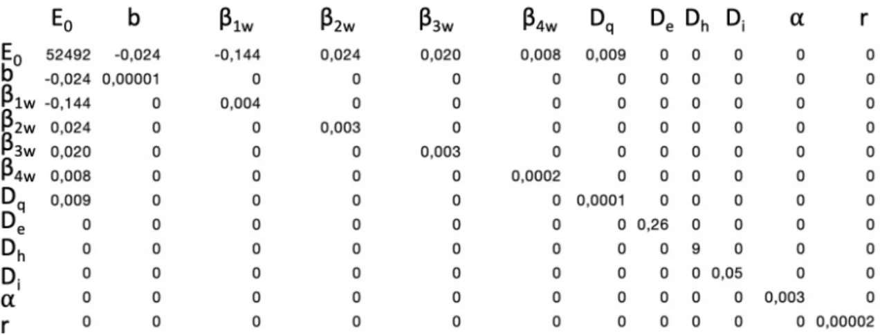
The seirah model and estimation of parameters has been extensively described in Prague et al. (2020). In this paper, to account for uncertainty in the model parameters, we use a distribution of models. At each episode, the epidemiological model is sampled from that distribution. The transition function is thus conditioned on a latent code (the model parameters) that is unknown to the agent. This effectively results in a stochastic transition from the viewpoint of the agent. To build the distribution of models, we assume a normal distributions for each of the model parameters, using either the standard deviation from the model inversion for parameters estimated in Prague et al. (2020) or 10% of the mean value for other parameters. Those values are available in appendix Figure 6 features for reproducibility of the experiment. We further add a uniformly distributed delay between the epidemic onset and the start of the learning episode (uniform in [0, 21 days]). This

delay models the reaction time of the decision authorities. This results in the distribution of models shown in Figure 7.

Appendix C. Additional Results

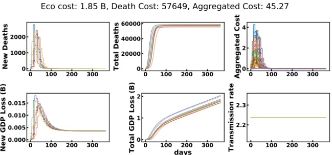
C.1 A Distribution of Models

Figure 7 presents the evolution of the seirah model states for a few models sampled from the distribution of models described in 4.1. Here, no lockdown is enforced.

0

100 200 300

0

1000

2000

New Deaths

0

100 200 300

0

20000

40000

60000

Total Deaths

0

₀

_{100 200 300}

2

4

Aggregated Cost

0

100 200 300

0.000

0.005

0.010

0.015

New GDP Loss (B)

0

0

100 200 300

_days

1

2

Total GDP Loss (B)

0

100 200 300

2.2

2.3

Transmission rate

Eco cost: 1.85 B, Death Cost: 57649, Aggregated Cost: 45.27

Figure 7: 10 models sampled from the distribution of epidemiological models used in the case-study.

Now, let us illustrate in details the results of the case study. C.2 Pareto Fronts Comparisons

Comparing multi-objective algorithms is not an easy task. The representation of the results itself is not trivial. Figure 4a, for example, presents the standard error of the mean in the GDP cost dimension, but cannot simultaneously represent the error in the other dimension. For this purpose, we can rotate the graph and present the standard error of the mean in the health cost dimension (see Figures 8a and 8b).

Statistical comparisons. We run each algorithm for 10 seeds to take into account the stochasticity of the learning process and assess the robustness of the algorithms. Rigor-ous algorithm comparison requires to compute statistical tests to assess the significance of differences in the mean performance (e.g. t-test, see Colas et al. (2019) for a discussion). Here, there are two dimensions resulting from the two costs. One way of handling this is to compare algorithms on one dimension, keeping the other constant. Figures 8a and 8b illustrate this process. In Figure 8a, the circles and stars evaluate the significance of differences (negative and positive w.r.t. the dqn performance respectively) in the economic cost dimension while the health cost is kept constant. In Figure 8b, we do the reverse and compare health costs, keeping economic costs constant.

0 10 20 30 40 50 60 # Deaths (×103₎ 0 50 100 150 200 GDP cost (B) NSGA-II (budget x15) GOAL DQN-C

NSGA-II (same budget)

(a) 0 25 50 75 100 125 150 175 GDP cost (B) 0 20 40 60 80 # D e a th s ( × 1 0 3) NSGA-II (budget x15) GOAL DQN-C

NSGA-II (same budget)

(b)

Figure 8: Pareto fronts for various optimization algorithms. Left: means and standard errors of the mean are computed in the economic cost dimension. right: they are computed in the health cost dimension (over 10 seeds). Stars indicate significantly higher performance w.r.t. the dqn condition while circles indicate significantly lower performance. We use a Welch’s t-test with level of significance α = 0.05.

Areas under the curve. One way to compare multi-objective algorithms is to compare the area under their normalized Pareto fronts (lower is better). We normalize all Pareto front w.r.t the minimum and maximum values on the two dimensions across all points from all experiments. We can then perform Welch’s t-tests to evaluate the significance of the difference between the mean areas metrics of each algorithm.

dqn goal dqn goal dqn-c nsga-ii (same) nsga-ii (x15)

dqn N/A 0.069 0.55 0.018 0.045

goal dqn N/A 0.046 0.84 0.0057

goal dqn-c N/A 0.21 0.35

nsga-ii (same) N/A 3.2 × 104

nsga-ii (x15) N/A

Table 2: Comparing areas under the Pareto fronts. The number in row i, column j compares algorithm i and j by providing the p-value of the Welch’s t-test assessing the significance of their difference. Bold colored numbers indicate significant differences, green indicate posi-tive differences (column algorithm performs better than row algorithm), while red indicate negative differences (column algorithm performs worse).

Now that we compared algorithms on average metrics, let us delve into each algorithm and look at particular runs to illustrate their respective strategies.

C.3 DQN

We first present strategies found by dqn.

0

100 200 300

1160

1180

1200

1220

S

(×

10

)

0

100 200 300

0

5

10

15

20

E

(×

10

)

0

100 200 300

0

100

200

300

400

I

0

100 200 300

20

40

60

80

R

(×

10

)

0

100 200 300

days

0

2

4

6

8

A

(×

10

)

0

100 200 300

0.0

0.5

1.0

H

(×

10

)

0

100 200 300

0

50

100

150

New Deaths

0

100 200 300

0

2000

Total Deaths

0.0

₀

_{100 200 300}

0.2

0.4

Aggregated Cost

0

100 200 300

0.4274

0.4276

0.4278

New GDP Loss (B)

0

0

100 200 300

_days

50

100

150

Total GDP Loss (B)

0

0

100 200 300

1

2

Transmission rate

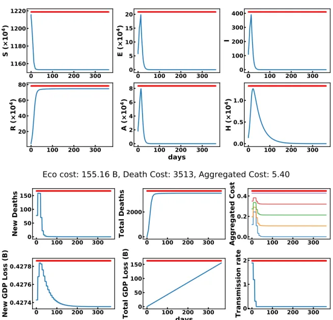
Eco cost: 155.16 B, Death Cost: 3513, Aggregated Cost: 5.40

Figure 9: dqn trained with β = 0.. For one run, this figure shows the evolution of model states (above) and states relevant for optimization (below). The aggregated cost is shown for various values of β in [0, 0.25, 0.5, 0.75, 1]. For β = 0, the agent only cares about the health cost, it always locks-down.

0

100 200 300

1217.5

1220.0

1222.5

1225.0

S

(×

10

)

0

100 200 300

0

1

2

3

E

(×

10

)

0

100 200 300

0

20

40

60

I

0

100 200 300

0

5

10

R

(×

10

)

0

100 200 300

days

0.0

0.5

1.0

A

(×

10

)

0

100 200 300

0.00

0.05

0.10

0.15

0.20

H

(×

10

)

0

100 200 300

0

10

20

New Deaths

0

100 200 300

0

200

400

600

Total Deaths

0

100 200 300

0.0

0.2

0.4

Aggregated Cost

0

100 200 300

0.0

0.2

0.4

New GDP Loss (B)

0

100 200 300

days

0

20

40

60

Total GDP Loss (B)

0

0

100 200 300

1

2

Transmission rate

Eco cost: 62.81 B, Death Cost: 556, Aggregated Cost: 31.84

Figure 10: dqn trained with β = 0.5. Here the strategy is cyclical with a one or two weeks period. For one run, this figure shows the evolution of model states (above) and states relevant for optimization (below). The aggregated cost is shown for various values of β in [0, 0.25, 0.5, 0.75, 1].