HAL Id: hal-03246076
https://hal.archives-ouvertes.fr/hal-03246076
Preprint submitted on 2 Jun 2021
HAL is a multi-disciplinary open access
archive for the deposit and dissemination of
sci-entific research documents, whether they are
pub-lished or not. The documents may come from
L’archive ouverte pluridisciplinaire HAL, est
destinée au dépôt et à la diffusion de documents
scientifiques de niveau recherche, publiés ou non,
émanant des établissements d’enseignement et de
On Data-Preparation Efficiency Application on Breast
Cancer Classification
Mouna Sabrine Mayouf, Florence Dupin de Saint Cyr - Bannay
To cite this version:
Mouna Sabrine Mayouf, Florence Dupin de Saint Cyr - Bannay. On Data-Preparation Efficiency
Application on Breast Cancer Classification. 2021. �hal-03246076�
Rapport IRIT n
° IRIT/RR–2020–09–FR
On Data-Preparation Efficiency
Application on Breast Cancer Classification
Mona Mayouf IRIT
Universit´
e Paul Sabatier
Toulouse, France
0000-0001-8714-0038
Florence Dupin de Saint-Cyr IRIT
Universit´
e Paul Sabatier
Toulouse, France
000-0001-7891-9920
May 31, 2021
Abstract
Quantifying the informative state of a dataset for a classification task is an important question. In this paper, we try to circumscribe this notion by introducing some new measures and enunciating some principles about data preparation. We experiment the interest of these measures and the validity of these principles by introducing several protocols designed for comparing different ways to prepare the data. We conclude by relating the efficiency of the data preparation and its theoretical diversity.
keywords: deep learning, convolutional neural networks, data prepa-ration, information metrics, Breakhis
1
Introduction
Affecting one in eight women in the world, breast cancer is one of the most com-mon cancer type acom-mong women, with one of the highest mortality rate [14]. In this context, convolutional neural networks (CNNs) have demonstrated remark-able accuracy and competitive reliability over traditional methods. However, according to [4], CNN approaches require that the network is trained on a huge amount of data. A main issue is that this amount is not always available: public datasets for a targeted task are not always available or does not have sufficient data. Besides, obtaining real data may be very expensive. Data-augmentation has been introduced to address this problem and has become one of the best-practices which improves the CNN results.
We should notice that the contribution of the artificial generation of data on the learning process is still poorly understood. Indeed, due to the CNN black-box aspect, it is difficult to identify how the data structure is guiding learning.
Is data augmentation successful just because it gives a redundancy which helps the learning? Is it necessary to provide fresh data or is it sufficient to generate data from old one? How can we quantify the information contained in a dataset for a given classification task? How the augmentation technique impacts the training process?
There has been an assumption that data augmentation is a mandatory standard step of data preparation. Traditional data-augmentation is based on basic image transformations that generate images extremely close to the initial data distribution space [17]. Other transformations (such as cut-out, Gaussian noising, Mix-up, overlapping) have been useful for some classification tasks [2] [3], [9]. With the success of generative adversarial networks (GANs), artificial fake images are generated [4]. However in critical fields such as health, where the information label must be conserved, there is a lot of restrictions on the possible transformations. Moreover, the lack of data which makes the learn-ing process unsuccessful can be associated with an imbalanced dataset, in which there is a glaring difference in the number of samples for a category compared to another. Depending on the classification task, this imbalanced rate may create a marginalised category during the training phase [13].
Through this article, we study how to quantify the amount of information in a dataset by first proposing several new measures, second enunciating a set of principles that should govern data-preparation (and help to answer some of the questions introduced abode), third designing several experimental protocols in order to check the validity of our set of principles, fourth experimenting them on BreakHis dataset (histopathological breast cancer images classified into benign and malignant).
2
Background
2.1
Classical information metrics
In this section, we first recall some metrics present in the literature. For this purpose, we consider a dataset D composed of n items, D = {s1, . . . , sn}, each item s being associated with a unique class c which is called the label of s and denoted by s.label = c. The set of possible classes is denoted C. Classically, the abundance aD(c) of a class c given a dataset D is the number of items of this class according to D, and the proportional abundance of a class c, PD(c), is the percentage of representation of a class among all the classes:
aD(c) = |{s ∈ D : s.label = c}| pD(c) =aDn(c)
According to [6], there are three indicators that have been defined in the liter-ature for estimating the diversity of a dataset, namely, the variety, the balance and the disparity. Here we expose some metrics aiming at capturing these indi-cators:
• Variety: The richness R is a metric related to the variety and represents the number of classes effectively considered for the classification task [5, 15]:
R(D) = |{c ∈ C : pD(c) > 0}|
• Balance: The imbalance ratio IR is the ratio of a majority over the minority classes in a binary classification [7]:
IR(D) = aD(Majority class) aD(minority class)
According to [8], the dataset is little imbalanced when 1.5 < IR < 3, medium imbalanced for 3 < IR < 9 and very imbalanced when IR > 9. Note that in the case of a binary classification, IR(D) = p 1
D(minority class)−
1. There are several other measures that capture the distribution of the data. However since they are all based on the proportional abundance p it means that they only take into account the number of items per class without considering the different natures of these items1.
• Disparity: The Disparity D quantifies the variety of the data based on a pairwise distance d between classes.
D =X
c∈C X
c0∈C
d(c, c0)
However providing the distance d between two classes requires additional knowledge (e.g. coming from the context of the classification task). Since Variety and Balance are only defined on the abundance of each class with respect to each other, the associated metrics will not help us very much in characterizing the quantity of information contained in the dataset. This is why in Section 4, we propose to introduce several new metrics based on Disparity or on the diameter of the dataset, that incorporates a distance d more appropriate for images.
2.2
BreakHis Dataset
“BreakHis” (which stands for “Breast Cancer Histopathological Database”) is a public dataset composed of 7909 histopathological biopsy images observed by four microscopic magnifications: 40X, 100X, 200X and 400X, collected from 82 patients by P&D Laboratory in Brazil on 2014 [14]. Among the labels that
1Three other measures could be considered, namely, Shannon entropy [12] H,
Herfindahl-Hirschman [11] HHI and Berger-Parker indexes BPI, which capture respectively the uncer-tainty in predicting the type of an item taken at random, the probability of two random items to belong to the same class and the maximal proportional abundance:
H(D) = −P
c∈CpD(c) × log(pD(c)) HHI(D) =Pc∈CpD(c)2
characterize the images, we focus on the tumor type which is either benign or malignant. This dataset is imbalanced with IR = 2.19 (see Table 1). Indeed, there are 2480 benign samples representing the minority, versus 5428 malignant ones, representing the majority category yielding a total amount of 7908 (only 5271 (i.e. 2/3) are used for the training phase, as explained in Section 7). In order to deal with this imbalanced dataset, we are going to propose several data-augmentation techniques and compare their impact on the learning process.
3
Formalisation and Protocols for BreakHis data
preparation
Data preparation consists in transforming the initial dataset in order to bet-ter train the network. Among the classical transformation, the more used are balancing and augmentation. Note that according to [13], there are three ways to rebalance the dataset : 1) over-sampling the minor class which amounts to augment the size of the minority class; 2) under-sampling the major class which consists in removing items from the majority class; 3) bagging the training phase which raises the probability to select an item in a marginalized category. The latter way to balance the data is out of the scope of this paper which focuses on data preparation techniques rather than training techniques.
This section first presents a list of principles that should hold when per-forming any data preparation, then we introduce the formalism adopted and the signature of the transformation functions that we are going to use for data augmentation. In order to validate the principles that we are introducing here, in Section 3.4 we have designed a discriminating set of experimental protocols whose results allow to confirm or deny these hypotheses.
3.1
General Principles for efficient data preparation
During data preparation, it is often the case that researchers use balancing techniques, or merely augment the data by doing some transformations on the samples. The best practices are guided by the results obtained, some practices are known to work better than others, however the hypothesis underlying the practices are not always made explicit. Moreover it is not clear if some practice are good or not, for instance sometimes augmentation creates duplicate of some samples, is it efficient to do so? Below, we enunciate a list of hypothetical prin-ciples that are inspired from the best practices in order to give more awareness about what should be a “rational data preparation”. Note that some of these principles are well known, and seem obvious and are still too fuzzy, however by writing them we show that more experiments are required for precising them. It also underlines the need for metrics that could characterize better the datasets, hence, justifying the work done in section 4. We can enunciate six principles that may improve the training:
• Sufficient Dataset Size (SDS) • No Duplication of Items (NDI)
• Well Chosen Transformation Operators (WCTO) • Variety of Transformation Operators (VTO) • Fresh External Data (FED)
Indeed, our experiments presented in Section 5 will confirm these rational principles. More precisely, (BD) stipulates that a balanced dataset behaves better than an unbalanced one for a classification task. (SDS) implies that a too small dataset may have a high negative impact (inefficiency and slow convergence) on the training process, even when the data is balanced. Moreover, by (NDI), we assume that duplication does not compensate the smallness of the dataset (it does not improve efficiency nor convergence). Furthermore, using data augmentation with no “fresh” data but with transformed items has often a positive impact on the training process, especially when the transformation is “label conservative”, this is the meaning of (WCTO). (WCTO) is also useful for balancing a dataset of sufficient size since by adding well transformed items to the minority class we can obtain a positive impact on training. Indeed we will see that some transformation perform better than others, obviously, label-conservative ones are mandatory. (VTO) expresses that using several diversified transformation operators has a positive impact. Finaly, adding fresh external real data perform better than adding generated data but may require more training time.
3.2
BreakHis transformation operators
In addition to the identity operator denoted Id, the data augmentation process is based on two types of elementary operators that are label-conservative (see [1] for the geometric operators and [16] for the color ones):
• Geometric operators Due to the fact that BreakHis images are rectangles of 460x700, any non-mirror geometric operation would yield a different shape which would need to be reshaped or cropped in order to feed the CNN. To avoid this post-operation that may decrease the precision, we opt for the only two operators that preserve the same shape: the horizontal and vertical flips. These two operators are denoted respectively H and V. • Color operators In order to increase the number of images, we consider also the possibility to play on colors. We use two operators: a RGB color inversion and a transformation of the RGB encoding of the image into the HSV color encoding. They are denoted respectively c and C.
In order to perform more than four distinct data augmentation, it is neces-sary to combine elementary operators by applying them successively. However, some combinations could create duplicated instances of the same images (e.g.
HV=VH, Hc=cH, ...). In summary, due to symmetries, only 15 distinct combi-nations are possible, namely: H, V, c, C, HV, Hc, HC, Vc, VC, cC, HVc, HVC, HcC, VcC, HVcC.
3.3
Signature of even split data-transformation
In this section, we introduce the signature of a particular kind of data transfor-mations with even distribution, i.e., the data is split into equal parts of samples where the same transformation is applied to all elements of the same part. Definition 1 (Signature). The signature of a even-split dataset transformation denoted tr(D, ops, ratio), is a function of the following parameters:
• D: the dataset to transform
• ops: the list of operators to apply to the different parts
• r: the division rate (in percentage) for splitting the dataset into parts (on which the operator(s) will apply)
where tr(D, (op1, . . . opp), r) = (op1(D1), . . . , opp(Dp)) is a partition of the dataset D into D1, . . . Dp (where p = 100/r) on which the operators (op1, . . . opp) are applied respectively and op(D) is an abbreviation for: op(D) = {op(s)|s ∈ D}
For instance we can consider the augmentation done by applying one el-ementary operation among (H, V, c, C) to each 25% of the dataset D: this augmentation has the signature tr(D, (H, V, c, C), 25). It consists in parti-tioning D into four parts (D1, D2, D3, D4) and apply H to D1, V to D2, c to D3 and C to D4 yielding a new dataset D0 = tr(D, (H, V, c, C), 25) = (H(D1), V (D2), c(D3), C(D4)).
Note that an augmentation that applies the same operator op to the whole dataset D has the following signature tr(D, (op), 100).
3.4
Experimental Protocols
In this section, we propose 13 different data preparation protocols for BreakHis dataset, designed with the purpose of enabling us to validate the General Prin-ciples enunciated above. D denotes the part of BreakHis dataset items assigned for training (we took 2/3 of the initial dataset) and Didenotes the new training dataset after preparation with the protocol Pi. In the following, all the samples s0 of Di are such that s0.label = s.label where s is the original sample in D which yields s0 in Di (by a transformation in {Id, H, V, C, c, HC, V c, CV, cH}). In other words the protocols are creating new samples that are labelled accord-ingly to their initial label in the original dataset.
BreakHis training Dataset D is composed of two classes, the marginal class called m, it is the benign category: m = {s ∈ D|s.label = benign}. The majority class denoted M is the malignant category: M = {s ∈ D|s.label = malignant}. Hence D = M ∪ m. Note that m has a size equal to half the size of
the majority class M , the protocols are using this characteristics for balancing the data.
1. Protocols 1 (no data creation): P1a is a control protocol where no bal-ancing nor augmentation are processed to the dataset. D1a = D; P1b is a second control protocol where only an augmentation is done without bringing “new” information: mere identical duplication of the items of the already majority class D1b = D ∪ tr(M, (Id), 100); P1c is a third control protocol which does not bring any “new” information but increases the size by simple duplication of the items in order to balance and augment the data D1c= D ∪ m ∪ tr(D ∪ m, (Id), 100).
2. Protocols 2 (balanced data) : double the size of the minority class with only one operator. P2auses a geometrical operator: D2a= D∪tr(m, (H), 100); P2b uses a color operator : D2b = D ∪ tr(m, (C), 100); P2c: balance by under-sampling. D2c = m ∪ Sample(M, |m|) where Sample(X, n) is a function that randomly selects n elements among the set X;
3. Protocols P3 (augmented unbalanced data) uses a color operator to aug-ment the size of the majority class : D3= D ∪ tr(M/2, (C), 100). 4. Protocols 4 (balanced and augmented data): with two single successive
operators. P4a uses the geometrical operators H and V : m0 = m ∪ tr(m, (H), 100) (double the size of the minority), D4a = M ∪ m0∪ tr(M ∪ m0, (V ), 100) (augment the whole dataset); P4b is similar to P4a but uses the color operators C and c; P4c uses the operators H and C; P4duses the operators V and c. P4euses the four operators applied on different parts of the dataset: m0 = m ∪ tr(m, (H, V, C, c), 25) (double the size of minority), D4e= M ∪ m0∪ tr(M ∪ m0, (C, c, V, H), 25) (augment2the whole dataset). P4f supply the lack of data by adding samples from another dataset3: D4f = M ∪ m ∪ m extra ∪ M extra where m extra (resp. M extra) is a set of 3|m| (resp.|M |) minority (resp. majority) category images of the other dataset.
4
Diversity measures
According to the definitions recalled in Section 2, in order to compute the dispar-ity D of a dataset, we should be able to provide a way to compute the distance between the different classes. We propose to define the distance between two classes by introducing first the distance between two images. Then we base the distance between two classes on the distance between the means of each classes. There are several ways to compute the distance between two images, for instance the Euclidean distance is based on a point-to-point comparison of the pixels of
2More precisely, D
4e = M ∪ m ∪ tr(m, (H, V, C, c), 25) ∪ tr(M, (C, c, V, H), 25) ∪
tr(m, (C, c, V, H), 25) ∪ tr(m, (HC, V c, CV, cH), 25)
each image (it is the norm of the matrix difference). Another idea is to take into account extra information in order to integrate into the distance the fact that horizontal and vertical symmetries should not increase the distance between images, because for a classification task these symmetries do not matter. This is why we choose to use a standard measure called SSIM (structural similarity index measure) [18] which estimates the similarity of two images based on a kind of contraction of the images according to their luminance, contrast and structure.
Definition 2 (SSI [18]). Let s1, s2 be two samples, SSI(s1, s2) =
(2µ1µ2+ α1)(2σ12+ α2) (µ2
1+ µ22+ α1)(σ21+ σ22+ α2)
where µ1, µ2, σ12, σ22, σ12, α1, α2 are the means and variance of s1.image and s2.image, the co-variance of s1.image and s2.image, and two small constants respectively.4.
Note that this similarity measure is invariant to the vertical and horizontal flip, since an image and its flipped version have the same average and variance. However this does not hold for color operation. We propose a SSI variant, called SSIC that is label-conservative for all operations introduced in Section 2.2, i.e., which is invariant to color operations c and C.
Definition 3. Let s1, s2 be two samples, SSIC(s1, s2) = min
op∈{Id,c,C}SSI(s1, op −1(s
2))
Example 1. for instance if s is a sample to be compared to its transformed sam-ple by RGB color inversion c(s), the distance SSIC(s, c(s)) is 0 since c−1(c(s)) = s
Proposition 1. For any combination cop of the elementary operators {Id, H, V , C, c}, it holds that for all sample s, SSIC(s, cop(s)) = 0
Proof. The proof concerning the geometric operators is due to the definition of SSI and is already explained in the Note below Definition 2. SSIC being built on SSI to ignore color transformations hence the result.
We are now in position to define the best representative sample among a set X, called µI(X). It is the sample which is the most similar to the other samples of X:
µI(X) = argmaxx∈X X
y∈X\{x}
SSIC(x, y)
We propose to evaluate the diversity of a dataset D by its disparity and diameter. The disparity has already been recalled above and is related to the
4These constants were introduced by [19] for avoiding unstability when the denominator
is close to 0 by setting α1= 0.01 × L and α2= 0.03 × L where L is the dynamic range of the
distinction between the different classes. The diameter is a general measure of the scope of the whole dataset independently of the classes, it is the maximum distance between any two images of the dataset. These two measures can be defined either on the Euclidean distance d, or on the more informed similarity measure SSIC yielding four measures diam, disp, diamI and dispI where I stands for “informed measure”. We normalize the Euclidean distance by the the greatest possible distance matrix denoted |im255|, i.e., the image composed of 255 on the three channels RGB (since the images are 460×700 then |im255| = √
460 × 700 × 3 × 2552= 250627.5125).
Definition 4. Given a dataset D, with two classes D1and D2 (D = D1∪ D2), • diam(D)= maxs1,s2∈Dd(s1.image,s2.image)
|im255|
• disp(D)= d(µ(D1),µ(D2))
|im255|
• diamI(D)=maxs1,s2∈D(1 − SSIC(s1.image, s2.image))
• dispI(D) = (1 − SSIC(µI(D1), µI(D2))
Note that concerning disparities, the definitions are given for a binary clas-sification (|C| = 2) where D1 is the part of the set D containing the first class and D2 is the part of the set containing the second class.5
The following proposition shows that all the protocols that we provide except P4f does not bring any “new” information to the dataset.
Proposition 2. for all the datasets Dij obtained by the protocols except D4f diamI(Dij) = diamI(D1a) and dispI(Dij) = dispI(D1a)
Proof. The proof is based on the invariance of SSIC wrt color and geometric operators.
5
Results and discussion
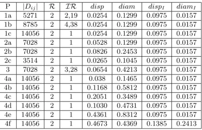
In this part, we try to estimate the amount of information that is contained in the different datasets obtained by the previous protocols. As said in Section 2, the variety and balance can be respectively estimated through the richness measure R and the imbalance ratio IR. This section evaluates the different protocols on two aspects, first the quantity of information present in the dataset produced by the protocol, second the classification efficiency given by a CNN trained on these datasets. Table 1 gives the different sizes Dij of the datasets obtained by the different protocols Pij. Note that the richness of the dataset obtained with any of the protocols remains the same since the number of classes remains constant: R(Dij) = 2 for all the datasets. Concerning the balance, the
5If there were more than two classes, the disparity would be 2P
c∈C
P
c0 ∈C\{c}d(µ(Dc),µ(Dc0))
imbalance ratio IR of the datasets Dij obtained by the different protocols is always 1 (due to the doubling of the size of the minority class that has a size equal to half the one of the majority class), for any protocol Pij except P1a, P1b and P3. Note that due to Proposition 2, the informed disparities and diameters are the same for all the datasets except D4f.
P |Dij| R IR disp diam dispI diamI 1a 5271 2 2,19 0.0254 0.1299 0.0975 0.0157 1b 8785 2 4,38 0.0254 0.1299 0.0975 0.0157 1c 14056 2 1 0.0254 0.1299 0.0975 0.0157 2a 7028 2 1 0.0528 0.1299 0.0975 0.0157 2b 7028 2 1 0.0826 0.2453 0.0975 0.0157 2c 3514 2 1 0.0265 0.1045 0.0975 0.0157 3 7028 2 3,28 0.0654 0.4213 0.0975 0.0157 4a 14056 2 1 0.038 0.1465 0.0975 0.0157 4b 14056 2 1 0.1168 0.5812 0.0975 0.0157 4c 14056 2 1 0.2051 0.3489 0.0975 0.0157 4d 14056 2 1 0.1030 0.4731 0.0975 0.0157 4e 14056 2 1 0.4361 0.8312 0.0975 0.0157 4f 14056 2 1 0.4673 0.4369 0.1385 0.2413
Table 1: Metrics Results obtained on BreakHis
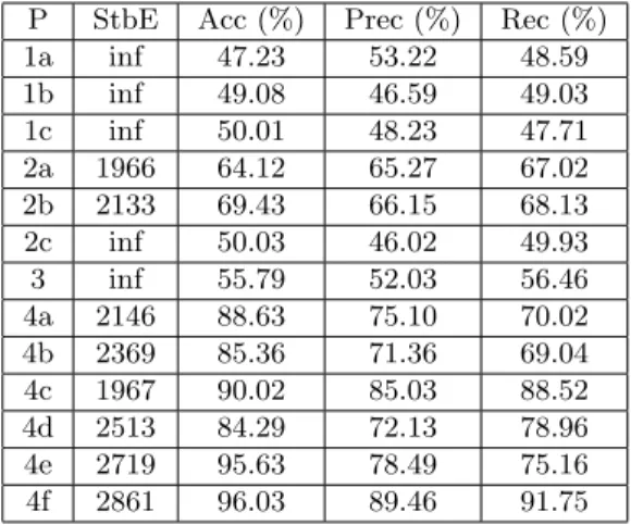
Table 2 describes the results obtained by the network trained on the datasets produced by the different protocols. Acc represents the accuracy, Acc is the rate of correctly classified samples among all the samples Acc = T M +T B+F M +F BT M +T B with T B (respectively T M , F B, F M ) denotes the number of samples correctly assigned to the benign (resp. correctly to the malignant, wrongly labeled benign, wrongly labeled malignant) class. Prec is the precision, it indicates the portion of correctly assigned elements among the ones that are predicted malignant P rec = T M +F MT M . Rec is the recall, it indicates the portion of samples correctly affected to the malignant class among all the samples that are malignant in the ground truth Rec =T M +F BT M . We also give an indication of the training behavior by mentioning the stabilization’s epoch StbE which is computed thanks to the early-stopping regularization technique [10]. It is the epoch from which the training loss is nearly steady. Table 3 shows the principles that seem to support the protocol performance, for WCTO and VTO we precise respectively the list of transformation operators and the number of distinct operators used.
In Table 2, the bad results of P1aand P2cunderlines that a too small dataset has a high negative impact on the training process, even when the data is balanced confirming the principle (SDS). Also, these two datasets had the smallest dispar-ity and diameters (absolute and informed). Having a small dispardispar-ity translates that the images of the two classes are near to each other making harder the discrimination task.
Duplication does not compensate the smallness of the dataset. Also, com-pensating the lack of data by duplicating identically the same images makes
P StbE Acc (%) Prec (%) Rec (%) 1a inf 47.23 53.22 48.59 1b inf 49.08 46.59 49.03 1c inf 50.01 48.23 47.71 2a 1966 64.12 65.27 67.02 2b 2133 69.43 66.15 68.13 2c inf 50.03 46.02 49.93 3 inf 55.79 52.03 56.46 4a 2146 88.63 75.10 70.02 4b 2369 85.36 71.36 69.04 4c 1967 90.02 85.03 88.52 4d 2513 84.29 72.13 78.96 4e 2719 95.63 78.49 75.16 4f 2861 96.03 89.46 91.75
Table 2: Accuracy Results obtained on BreakHis
P BD SDS NDI WCTO (ops) VTO (nb ops) FED 1a no no yes no 0 no 1b no no no no 0 no 1c yes yes no no 0 no 2a yes no yes H 1 no 2b yes no yes C 1 no 2c yes no yes no 0 no 3 no no yes C 1 no 4a yes yes yes V + VH 2 no 4b yes yes yes c + cC 2 no 4c yes yes yes C + CH 2 no 4d yes yes yes c + cV 2 no
4e yes yes yes C + c + V + H
+ CH + cV + VC + Hc
8 no
4f yes yes yes no 0 yes
Table 3: Principles satisfied by the protocols
the training even more difficult and yields the CNN into over-fitting (P1b and P1c), because for these latter protocols the CNN is unstable and blocked in a transitory regime with a bad accuracy under 50%, confirming the (NDI) princi-ple. Using data augmentation with no “fresh” data but with transformed items has a positive impact on the training process (since P4a gives better results than P1cand P2bbeing better than P2c) this confirms both (WCTO) and (BD) principles. Moreover, the reader can check that augmenting a balanced dataset increases the performances, (see P4abcdef wrt P2abc) which supports again the (SDS) and (BD) principles. Note that the color transformations have better impact than the geometric ones (P2b being better than P2a and P4c than P4a), consolidating the (WCTO) principle. In parallel, we observe that both the
dis-parity and the diameter are augmented by adding transformed samples relating these measure to the (WCTO) and (VTO) principles. In addition, we conclude that varying the operators by using them on different parts of the dataset, in-creases the accuracy : the best accuracy 95.63% is obtained in that case (P4e) with the use of 8 different operators demonstrating the importance of (VTO) principle which is again correlated with a high disparity and diameter. Lastly, we see that P4f has the best performances with the addition of fresh external data (FED) but this protocol needs more training time. Obviously having the possibility to add fresh external data is ideal, however, it is not always possi-ble to find more real data, this is why we can consider that P4e and P4c are the best data preparations. Contrarily to what was expected, several dataset that have equal values with dispI and diamI may have very different efficiency. These measures are capturing a kind of brute richness similar to the one that a human expert could have given by understanding the equivalences between samples. It seems that the network is benefiting from the creation of equivalent samples which do not increase what we call “informed” disparity and diameter but increase the non informed disparity and diameter.
6
Conclusion
This article studies the data preparation process through the idea that there is a need for evaluating the quantity of information present in a dataset in terms of efficiency for a classification task. For this purpose, we define four new metrics to evaluate the dataset diversity and we formalize six rational principles for data preparation. Then, we experiment 13 data-preparation protocols and identified among them the most suitable ones for BreakHis images classification. As a perspective of this work we propose to use the saliency maps technique to visualize what the CNN is considering from a transformed data and to define another family of informativeness metrics.
7
Ethical Issues and Computational Details
This research study was conducted retrospectively using human subject data made available in open access and ethically approved by (https://www.kaggle. com/ambarish/breakhis).
We used the pre-trained ”VGG19” convolutional neural network model as a classifier to compare the different dapa-preparation protocols. In order to optimize the network training, we used the the several regularization techniques such as the L2 regularization with α set to 0.01, the early stopping and the dropout techniques are also used. We trained our model for 3000 epochs with a batch size of 64. We opted for Adam-optimiser for a learning rate fixed initially at 0.0001. The initial breakHis dataset was split into 2/3 for the training set D1a, 1/6 for validation and 1/6 for the test. |D1a| = 5271, p(M ) = 2/3, p(B) = 1/3
8
Acknowledgments and Ethical Issues
This research study was conducted retrospectively using human subject data made available in open access and ethically approved by (https://www.kaggle. com/ambarish/breakhis). The authors have non-financial interests to dis-close. Experiments presented in this paper were carried out using the OSIRIM platform that is administered by IRIT and supported by CNRS, the R´egion Midi-Pyr´en´ees, the French Government, ERDF (see https://osirim.irit. fr/site/en).
References
[1] Teresa Ara´ujo, Guilherme Aresta, Eduardo Castro, Jos´e Rouco, Paulo Aguiar, Catarina Eloy, Ant´onio Pol´onia, and Aur´elio Campilho. Classifica-tion of breast cancer histology images using convoluClassifica-tional neural networks. PloS one, 12(6), 2017.
[2] Anderson de Andrade. Best practices for convolutional neural networks applied to object recognition in images. arXiv preprint arXiv:1910.13029, 2019.
[3] Terrance DeVries and Graham W Taylor. Improved regularization of con-volutional neural networks with cutout. arXiv preprint arXiv:1708.04552, 2017.
[4] Ian Goodfellow, Yoshua Bengio, and Aaron Courville. Deep learning. MIT press, 2016.
[5] Robert H MacArthur. Patterns of species diversity. Biological reviews, 40(4):510–533, 1965.
[6] Pedro Ramaciotti Morales, Robin Lamarche-Perrin, Raphael Fournier-S’niehotta, Remy Poulain, Lionel Tabourier, and Fabien Tarissan. Mea-suring diversity in heterogeneous information networks. arXiv preprint arXiv:2001.01296, 2020.
[7] Albert Orriols-Puig and Ester Bernad´o-Mansilla. Bounding xcs’s param-eters for unbalanced datasets. In Proc. of the 8th annual conference on Genetic and evolutionary computation, pages 1561–1568, 2006.
[8] Albert Orriols-Puig and Ester Bernad´o-Mansilla. Evolutionary rule-based systems for imbalanced data sets. Soft Computing, 13(3):213, 2009. [9] Daniel S Park, William Chan, Yu Zhang, Chung-Cheng Chiu, Barret Zoph,
Ekin D Cubuk, and Quoc V Le. Specaugment: A simple data augmentation method for automatic speech recognition. arXiv preprint arXiv:1904.08779, 2019.
[10] Lutz Prechelt. Early stopping-but when? In Neural Networks: Tricks of the trade, pages 55–69. Springer, 1998.
[11] Stephen A Rhoades. The herfindahl-hirschman index. Fed. Res. Bull., 79:188, 1993.
[12] Claude E Shannon. A mathematical theory of communication. The Bell system technical journal, 27(3):379–423, 1948.
[13] Connor Shorten and Taghi M Khoshgoftaar. A survey on image data aug-mentation for deep learning. Journal of Big Data, 6(1):1–48, 2019. [14] Fabio Alexandre Spanhol, Luiz S Oliveira, Caroline Petitjean, and Laurent
Heutte. Breast cancer histopathological image classification using convo-lutional neural networks. In 2016 international joint conference on neural networks (IJCNN), pages 2560–2567. IEEE, 2016.
[15] Andrew Stirling. On the economics and analysis of diversity. Science Policy Research Unit (SPRU), Electronic Working Papers Series, Paper, 28:1–156, 1998.
[16] David Tellez, Geert Litjens, P´eter B´andi, Wouter Bulten, John-Melle Bokhorst, Francesco Ciompi, and Jeroen van der Laak. Quantifying the effects of data augmentation and stain color normalization in convolu-tional neural networks for computaconvolu-tional pathology. Medical image analy-sis, 58:101544, 2019.
[17] David A Van Dyk and Xiao-Li Meng. The art of data augmentation. J. of Comp. and Graphical Statistics, 10(1):1–50, 2001.
[18] Zhou et al. Wang. Multiscale structural similarity for image quality assess-ment. In The Thrity-Seventh Asilomar Conference on Signals, Systems & Computers, 2003, volume 2, pages 1398–1402. Ieee, 2003.
[19] Wang Zhou. Image quality assessment: from error measurement to struc-tural similarity. IEEE Trans. image proc., pages 600–613, 2004.