THE CHARACTERIZATION OF SEISMIC EARTH STRUCTURES AND NUMERICAL MANTLE CONVECTION EXPERIMENTS
USING TWO-POINT CORRELATION FUNCTIONS
by
PETER PUSTER
Vordiplom in Geophysik, Universitat Fridericiana, Karlsruhe, 1986 Submitted to the Department of
Earth, Atmospheric, and Planetary Sciences
in partial fulfillment of the requirements for the degree of
DOCTOR OF PHILOSOPHY at the
MASSACHUSETTS INSTITUTE OF TECHNOLOGY February 1995
© Massachusetts Institute of Technology 1995 All rights reserved
Signature of Aunthor_________________
Department of Earth, Atmospheric, and Planetary Sciences
Il. November, 1994 Certified b, Thomas H. Jordan Thesis Supervisor Certified by Bradford H. Hager Thesis Co-Supervisor Accepted by Thomas H. Jordan Department Head
Wi1T
UAWN
FROM
M1tL
IR
i E
uthor_
.
_
I --/7)
-- -THE CHARACTERIZATION OF SEISMIC EARTH STRUCTURES
AND NUMERICAL MANTLE CONVECTION EXPERIMENTS USING Two-POINT CORRELATION FUNCTIONS
PETER PUSTER
Submitted to the Department of Earth, Atmospheric, and Planetary Sciences in partial fulfillment of the requirements for the degree of Doctor of Philosophy
ABSTRACT
We consider a time-dependent random field, f(rZt), defined on a spherical shell [Q=(6,q), O56 , -t<(p it] or cylindrical annulus [92=P, -1E<(P57r]. Examples are the temperature distribution, T(r,2,t), or the radial component of the flow velocity, u(r,2,t), obtained from numerical simulations of high Rayleigh number convection. For such a field the spatio-temporal two-point correlation function, Cff(r,r',A,t*), is constructed by averaging over rotational transformations of this ensemble. To assess the structural differences among mantle convection experiments we construct three spatial subfunctions of Cif(r,r',A,t*): the rms variation, af(r) =
Cf(r,r,0,0), the radial correlation function, Rf(r,r?) = Cf(r,r' ,0,0) / af(r) aj(r'),
and the angular correlation function, Af(r,A) = Cff(rr,A,0)/ a 2(r). The integral
transform of Af(r,A) is the angular power spectrum. Rf(r,r') and Af(r,A) are symmetric about the loci r = r' and A =0, respectively, where they achieve their maximum value of unity. The fall-off of Rf and Af away from their symmetry axes can be quantified by a correlation length pf(r) and a correlation angle af(r), which we define to be the halfwidths of the central peaks at the correlation level 0.75. The behavior of pf is a diagnostic of radial structure, while af measures average plume width.
We use two-point correlation functions of the temperature field (T-diagnostics) and flow velocity fields (V-diagnostics) to quantify some important aspects of mantle convection experiments. We explore the dependence of different correlation diagnostics on Rayleigh number, internal heating rate, radial viscosity variations, temperature-dependent rheology, phase changes, and plates. For isoviscous flows in an annulus, we show how radial averages of UT, pr, and aT scale with Rayleigh number for various internal heating rates. A rapid 10-fold to 30-fold viscosity increase with depth yields weakly stratified flows, quantified by q., which is a measure of radial flux. The horizontal flux diagnostic a,, reveals that the flow organization is sensitive to the depth of the viscosity increase. We illustrate that T-diagnostics, which are more easily relatable to geophysical observables, can serve as proxies for the V-diagnostics. A viscosity increase with depth is evident as an increase in the T-diagnostics in the high-viscosity region. For numerical experiments with a temperature-dependent rheology we employ a mobilization scheme for the upper boundary layer. Temperature dependence does not appreciably perturb the a-diagnostics or aT in the convecting interior. Changes in the radial correlation length are two-fold. First, the greater viscosity of cold downwellings
leads to an increase in height and width of the radial correlation maximum near the top. Second, the increase in pT associated with a viscosity jump is markedly reduced. An endothermic phase transition manifests itself in the correlation diagnostics as a local minimum in a, and pT and local maxima in UT and aT around the phase transition depth. Temperature-dependent rheology reduces the amount of layering, however, the phase-change induced layering is still apparent in the two-point correlation diagnostics. When the phase change coincides with a rapid viscosity increase the effects of the latter dominate. We investigate the influence of surface plates on the organization of mantle flow. Plates whose geometries evolve with time are modeled by using a temperature-dependent viscosity combined with weak zones (small regions of low viscosity) advected by the flow. The two-point correlation diagnostics obtained from these flows are similar to the temperature-dependent runs with a mobilized upper boundary layer. Differences include an increase in au and aT near the surface, and a shift of the maximum in a. to shallower depths. The main influence of plates is to organize the large-scale flow structure. This is best documented in the angular power spectrum, which has more power concentrated at low wavenumbers. We also quantify some statistics of the plate system, such as plate-size and relative plate-velocity distributions. Average plate velocities decrease nearly monotonically with increasing plate size for cases without a viscosity stratification. Viscously stratified systems exhibit a more uniform average plate-velocity distribution. Comparing plate system statistics from numerical convection calculations to the plate tectonic record for the past 120 Ma favors models with a 30-fold viscosity increase in the lower mantle over those with a viscosity that is constant with depth.
We calculate the two-point moment functions for global and regional models of seismic shear velocity heterogeneity, 8#(r,.2). The radial correlation function is least sensitive to the low-pass filtering required when comparing convection experiments to low-resolution seismic images, making it the most useful tool for comparisons between the two. As long as thermal anomalies are predominantly responsible for seismic velocity heterogeneity, a direct comparison between pr and pp is meaningful. We find significant differences between the tomographic models, which frustrate a detailed interpretation of individual features of pp. The overall morphology of the pp-profiles, however, whereas consistent with pT curves for convection models with a 30-fold to
100-fold viscosity increase at 670 km depth, rules out convection models with a viscosity that is constant with depth. We define stratification indices for the radial correlation length, S(p), and average radial flux, S(lul), at 670 km depth. Using stratification values for the seismic models (S(pp) 0.12), we infer S(ul) 0.1, indicating that the present-day style of convection is dominantly whole-mantle. Together with A(ias), a measure of the asymmetry of the radial flux distribution at 670 km depth, S(Iul) furthermore
suggests that it is unlikely for the earth to be in an intermittently layered regime.
Thesis committee:
Dr. Thomas H. Jordan, Professor of Geophysics (thesis supervisor) Dr. Bradford H. Hager, Professor of Geophysics (thesis co-supervisor) Dr. Daniel H. Rothman, Professor of Geophysics
Dr. John Grotzinger, Professor of Geology
Table of contents
Dedication
3
Abstract
5
Table of contents
7
Chapter 1
Introduction
9
References 13Chapter 2 Two-point correlation functions
Introduction 17 Definitions 18 Example calculation 21 Geometry 25 References 29 Figure Captions 31 Figures 33
Chapter 3 Convection models
Introduction 43
Scaling relationships 43
Depth- and temperature-dependent viscosity 46
Phase transitions 53 Supercontinents 57 Evolving plates 59 Discussion 66 References 70 Tables 73 Figure Captions 78 Figures 89
Chapter 4 Tomographic earth structures
Introduction 125
Global tomographic models 126
Model resolution and parameterization 130
Filtering 132
Regional tomographic models 134
Discussion 136
References 139
Figure Captions 141
8
Chapter 5 Summary and Conclusions 169
References 177
Figure Captions 178
Figures 180
Appendix A Field equations of mantle convection
Formulation 187
References 190
Tables 191
CHAPTER
1
INTRODUCTION
One goal of structural seismology is to map the aspherical variations in the seismic
wave speeds in sufficient detail to resolve diagnostic properties of the mantle convection. The most fundamental issue, posed forty-three years ago by Birch [1951], is the degree to
which the large-scale flow is stratified by changes in mineralogical phase and/or bulk
chemistry across the mid-mantle transition zone from depths of 400 to 700 km. The first data on seismic heterogeneity directly addressing this issue became available in the mid-1970's through early attempts to detect the penetration of cold, subducted lithosphere into the lower mantle beneath zones of plate convergence [Jordan and Lynn, 1974; Jordan, 1977]. Recent tomographic studies of subduction zones in the western Pacific [van der Hilst et al., 1991; Fukao et al., 1992] and beneath the Americas [Grand, 1987; Grand,
1994] have confirmed the existence of high-velocity anomalies, presumably slab-related, extending below the 660-km seismic discontinuity in several subduction regions. In other locations, however, tomographic images seem to reveal near-horizontal high-velocity anomalies above 660 km, interpreted as slabs deflected sideways by the interface [van der Hilst et al., 1991; Fukao et al., 1992]. Because of these apparent complexities in the seismic data pertaining to the deep structure of subduction zones, no consensus has yet developed regarding the extent to which the 660-km discontinuity forms a barrier to
mantle flow [Olson et al., 1990].
The most plausible mineralogical explanation for the jump in elastic parameters at the 660-km discontinuity is the endothermic dissociation of spinel-structured (Mg,Fe)2SiO4 (y-olivine) into (Mg,Fe)O (magnesiowiistite) plus perovskite-structured (Mg,Fe)SiO3.
Laboratory measurements of the Clapeyron slope, y, for the spinel -post-spinel transition yield values of -2.8 MPa/K [Ito and Takahashi, 1989] and -3±1 MPa/K [Akaogi and Ito, 1993]. Convection calculations incorporating phase-change dynamics with
two-dimensional [Christensen and Yuen, 1985; Machetel and Weber, 1991; Peltier and Solheim, 1992; Zhao et al., 1992] and three-dimensional [Honda et al., 1993; Tackley et al., 1993; Tackley et al., 1994] flow geometries indicate that an endothermic transition of this magnitude acts to inhibit convection through the phase boundary.
The 660-km discontinuity could also mark a compositional boundary between the upper and lower mantle [Richter and Johnson, 1974], at least in some average sense [Jeanloz, 1991]. The strongest evidence favoring a chemical difference is a discrepancy between the lower-mantle density profile predicted for an upper-mantle (pyrolitic) composition and the seismically determined density profile. According to some studies [Jeanloz and Knittle, 1989; Stixrude et al., 1992], the former is 3-7% lower than the latter, implying an increase in either the iron/magnesium ratio or the silica content of the lower mantle, or both (see, however, Chopelas and Boehler [1992]). Numerical simulations suggest that a density difference near the upper end of this range would imply layered convection with deformation of the chemical boundary but very little mass exchange [Christensen and Yuen, 1984], while a density contrast near the lower end might be maintained by some form of penetrative convection [Christensen and Yuen, 1984; Silver et al., 1988]. The seismic mapping of subduction zones has been sufficiently ambiguous that compositionally stratified models-even the end-member hypothesis of layered convection-remain in contention.
Another mechanism for impeding vertical flow is an increase of viscosity with depth. Most radial viscosity structures obtained from modeling the earth's non-hydrostatic geoid [Hager et al., 1985; Hager and Richards, 1989; Ricard and Wuming, 1991; King and Masters, 1992; Forte et al., 1993] exhibit a rapid viscosity increase from the upper to the lower mantle.
Seismic observations have been a principal tool for probing the earth's deep interior and addressing questions regarding the organization of convection currents in the mantle. Global maps of mantle shear-wave velocity heterogeneity,
31,
[e.g., Tanimoto, 1990; Masters et al., 1992; Su et al., 1992] provide snapshots of mantle dynamics, assuming that 8# is proportional to convectively induced temperature anomalies ST. (Thisassumption should be a good working hypothesis in the mantle's interior away from the chemical boundary layers at the free surface and core-mantle boundary.) Numerical convection experiments, on the other hand, give insight into the dynamics of the mantle flow system. Because our understanding of mantle convection is still crude, numerical simulations cannot reproduce the exact geographical details, but only the grosser aspects of the flow pattern. Therefore, quantification schemes that measure the effect of different parameters on convective flow organization and structure are necessary. Examples of flow diagnostics are the angular power spectrum [e.g. Jarvis and Peltier, 1986; Tanimoto, 1990] and the root-mean-square (rms) variation on horizontal surfaces [Honda, 1987]. Recently, Jordan et al. [19931 and Puster and Jordan [1994] have introduced two-point correlation diagnostics, the radial and angular correlation functions, that are invariant with respect to the temperature coefficient of shear-wave speed, (d# / dT)p, and thus well-suited for comparison to seismic observations.
In chapter 2 we introduce the complete spatio-temporal two-point correlation functions of the temperature and flow velocity fields as tools for studying high-Rayleigh number fluid flow and illustrate the concepts with an example calculation of infinite Prandtl number thermal convection in a cylindrical annulus. We also investigate the influence of geometry on the flow by quantifying the second-order statistics of 2D and
3D convection calculations.
Chapter 3 applies this formalism to characterize the second-order statistics of mantle convection experiments encompassing a large number of different effects. In particular, we quantify the effects of Rayleigh number and internal heating rate and present scaling relations for different correlation diagnostics. We also investigate the influence of both depth-dependent and depth- and temperature-dependent viscosities on flow structure and correlation functions. A lot of recent attention has been paid to mantle flow models incorporating the effects of phase changes. We show that two-point correlation functions are sensitive indicators of the degree of flow stratification due to an endothermic phase boundary. The influence of surface plates on the mantle flow is another important effect.
We present flow models of rigid surface plates, whose geometries evolve with time and characterize the second-order properties of the resulting flow fields.
In chapter 4 we quantify the second-order properties of several recent global and regional seismic earth models. As global tomographic models can only constrain the large-scale pattern of mantle flow it is important to investigate the effects of filtering on two-point correlation diagnostics. We also address the issues of model resolution and model parameterization. Using two-point correlation functions also allows us to quantitatively compare the different seismic structures.
Chapter 5 gives a brief summary of the main results of chapters 3 and 4 and discusses some implications about the importance of various effects on the style of mantle convection.
REFERENCES
Akaogi, M., and E. Ito, Refinement of enthalpy measurement of MgSiO3 perovskite and negative pressure-temperature slopes for perovskite-forming reactions, Geophys. Res. Lett., 20, 1839-1842, 1993.
Birch, F., Remarks on the structure of the mantle, and its bearing upon the possibility of convection currents, Trans. Am. Geophys. Union, 32, 533-534, 1951.
Chopelas, A., and R. Boehler, Thermal expansivity in the lower mantle, Geophys. Res. Lett., 19, 1347-1350, 1992.
Christensen, U. R., and D. A. Yuen, The interaction of a subducting lithospheric slab with a chemical or phase boundary, J. Geophys. Res., 89, 4389-4402, 1984.
Christensen, U. R., and D. A. Yuen, Layered convection induced by phase transitions, J.
Geophys. Res., 90, 10, 1985.
Forte, A. M., A. M. Dziewonski, and R. L. Woodward, Aspherical structure of the mantle, tectonic plate motions, nonhydrostatic geoid, and topography of the
core-mantle boundary, in Dynamics of Earth's deep interior and Earth rotation, edited by J. L. LeMouel, D. E. Smylie, and T. Herring, Geophysical Monograph, 72, pp.
135-166, 1993.
Fukao, Y., M. Obayashi, H. Inoue, and M. Nenbai, Subducted slabs stagnant in the mantle transition zone, J. Geophys. Res., 97,4809-4822, 1992.
Grand, S. P., Tomographic inversions for shear structure beneath the North American plate, J. Geophys. Res., 92, 14065-14090, 1987.
Grand, S. P., Mantle shear structure beneath the Americas and surrounding oceans, J. Geophys. Res., 99, 11591-11621, 1994.
Hager, B. H., R. W. Clayton, M. A. Richards, R. P. Comer, and A. M. Dziewonski, Lower mantle heterogeneity, dynamic topography and the geoid, Nature, 313, 541-545, 1985.
Hager, B. H., and M. A. Richards, Long-wavelength variations in Earth's geoid; physical models and dynamical implications, Philos. Trans. R. Soc. London, Ser. A, 328, 309-327, 1989.
Honda, S., The RMS residual temperature in the convecting mantle and seismic heterogeneities, J. Phys. Earth, 35, 195-207, 1987.
Honda, S., D. A. Yuen, S. Balachandar, and D. Reuteler, Three-dimensional instabilities of mantle convection with multiple phase transitions, Science, 259, 1308-1311, 1993. Ito, E., and E. Takahashi, Postspinel transformations in the system Mg2SiO4-Fe2SiO4
and some geophysical implications, J. Geophys. Res., 94, 10637-10646, 1989.
Jarvis, G. T., and W. R. Peltier, Lateral heterogeneity in the convecting mantle, J. Geophys. Res., 91, 435-451, 1986.
Jeanloz, R., Effects of phase transitions and possible compositional changes on the seismological structure near 650 km depth, Geophys. Res. Lett., 18, 1743-1746, 1991.
Jeanloz, R., and E. Knittle, Density and composition of the lower mantle, Philos. Trans. R. Soc. London, Ser. A, 328, 377-389, 1989.
Jordan, T. H., Lithospheric slab penetration into the lower mantle beneath the Sea of Okhotsk, J. Geophys., 43, 473-496, 1977.
Jordan, T. H., and W. S. Lynn, A velocity anomaly in the lower mantle, J. Geophys. Res., 79, 2679-2685, 1974.
Jordan, T. H., P. Puster, G. A. Glatzmaier, and P. J. Tackley, Comparisons between seismic Earth structures and mantle flow models based on radial correlation functions, Science, 261, 1427-1431, 1993.
King, S. D., and T. G. Masters, An inversion for radial viscosity structure using seismic tomography, Geophys. Res. Lett., 19, 1551-1554, 1992.
Machetel, P., and P. Weber, Intermittent layered convection in a model mantle with an endothermic phase change at 670 km, Nature, 350, 55-57, 1991.
Masters, T. G., H. Bolton, and P. Shearer, Large-scale 3-dimensional structure of the mantle, Eos Trans. AGU, 73, 201, 1992.
Olson, P., P. G. Silver, and R. W. Carlson, The large-scale structure of convection in the Earth's mantle, Nature, 344, 209-215, 1990.
Peltier, W. R., and L. P. Solheim, Mantle phase transitions and layered chaotic convection, Geophys. Res. Lett., 19, 321-324, 1992.
Puster, P., and T. H. Jordan, Stochastic analysis of mantle convection experiments using two-point correlation functions, Geophys. Res. Lett., 21, 305-308, 1994.
Ricard, Y., and B. Wuming, Inferring the viscosity and 3-D density structure of the mantle from geoid, topography and plate velocities, Geophys. J. Int., 105, 561-571, 1991.
Richter, F. M., and C. E. Johnson, Stability of a chemically layered mantle, J. Geophys. Res., 79, 1635-1639, 1974.
Silver, P. G., R. W. Carlson, and P. Olson, Deep slabs, geochemical heterogeneity, and the large-scale structure of mantle convection; investigation of an enduring paradox, Ann. Rev. Earth Planet. Sci., 16, 477-541, 1988.
Stixrude, L. S., R. J. Hemley, Y. Fei, and H. K. Mao, Thermoelasticity of silicate perovskite and magnesiowustite and stratification of the earth's mantle, Science, 257, 1099-1101, 1992.
Su, W.-J., R. L. Woodward, and A. M. Dziewonski, Joint inversions of travel-time and waveform data for the 3-D models of the Earth up to degree 12, Eos Trans. AGU, 73, 201, 1992.
Tackley, P. J., D. J. Stevenson, G. Glatzmaier, and G. Schubert, Effects of an endothermic phase transition at 670 km depth in a spherical model of convection in the Earth's mantle, Nature, 361, 699-704, 1993.
Tackley, P. J., D. J. Stevenson, G. A. Glatzmaier, and G. Schubert, Effects of multiple phase transitions in a 3-D spherical model of convection in the Earth's mantle, J. Geophys. Res., 99, 15877-15901, 1994.
Tanimoto, T., Long-wavelength S-wave velocity structure throughout the mantle,
15
van der Hilst, R. D., R. Engdahl, W. Spakman, and G. Nolet, Tomographic imaging of subducted lithosphere below Northwest Pacific island arcs, Nature, 353, 37-43, 1991. Zhao, W., D. A. Yuen, and S. Honda, Multiple phase transitions and the style of mantle
CHAPTER
2
TWO-PoINT CORRELATION FUNCTIONS
INTRODUCTION
Seismic observations have been a principal tool for probing the earth's deep interior and addressing questions regarding the organization of convection currents in the mantle. The features of mantle shear-wave velocity heterogeneity, 8#, are now being mapped on a global scale with increasing precision and resolution [e.g., Tanimoto, 1990; Masters et al., 1992; Su et al., 1994] provide snapshots of mantle dynamics, assuming that
S#
is proportional to convectively induced temperature anomalies ST. This should be a good approximation in the interior away from the boundary layers, but it is invalid in the uppermost mantle, where the continental chemical boundary layer exerts a strong control on aspherical heterogeneity [Jordan, 1981], and perhaps at the base of the mantle, where chemical heterogeneity may also dominate [Jordan, 1979; Lay, 1989]. Numerical convection experiments, on the other hand, give insight into the dynamics of the mantle flow system. Because mantle convection is spatially and temporally chaotic [e.g., Vincent and Yuen, 1988] and our understanding of mantle dynamics is still crude, numerical simulations cannot reproduce the exact geographical details, but only the grosser aspects of the flow pattern. Therefore, quantification schemes that measure the effect of different parameters on convective flow organization and structure are necessary. Attention has thus far been focused primarily on power spectra [e.g. Jarvis and Peltier, 1986; Tanimoto, 1990] and the root-mean-square (rms) variation on horizontal surfaces [Honda, 1987]. Recently, Jordan et al. [1993] and Puster and Jordan [1994] have introduced two-point correlation diagnostics, the radial and angular correlation functions, that are invariant with respect to the temperature coefficient ofshear-wave speed, (0# / dT)p, and thus well-suited for comparison to seismic
observations.
The spatial two-point correlation functions are useful for capturing the flow characteristics of mantle convection experiments in a succinct yet comprehensive manner. Instead of gigabytes of snapshots of the time-dependent flow field, useful for obtaining qualitative insight into a convective system, two-point correlation functions provide a means for quantitative analysis of a flow regime that can be directly compared to seismic observations.
A statistical approach for analyzing fluid flow has been used for many years in the study of turbulence (see Monin and Yaglom [1971; 1975] for a comprehensive summary). The focus of statistical fluid mechanics has been on moment functions, or equivalently power spectral densities, arising from a stochastic analysis of the equations of fluid dynamics. The simplest examples are the Reynolds equations, which are derived by ensemble-averaging the Navier-Stokes equations for an incompressible fluid. Moments arising in this context are, for example, the mean velocity, (v(r,t)), or the covariance of velocity fluctuations, (3v;(r,t)8vj(r' ,t)). The fundamental problem arising from statistical averaging of the momentum equations is that any finite system of equations contains more unknowns than equations (a problem referred to as the closure problem in the turbulence literature) and is thus unsolvable. We, therefore, determine the statistical properties of the flow by analyzing numerical solutions of the primitive equations instead. In the following section we introduce the complete spatio-temporal two-point correlation functions of the temperature and flow velocity fields as tools for studying high-Rayleigh number fluid flow and illustrate the concepts with an example calculation of infinite Prandtl number thermal convection in a cylindrical annulus.
DEFINITIONS
We consider a time-dependent random field, f(r, S2, t), defined on a spherical shell [S2=(e,(P), 0 19 , -ir<(p r] or cylindrical annulus [=p, -x <p 5ic]
extending over a radial interval b r 1. Examples are the temperature distribution, T(r,2,t), or the radial component of the flow velocity, u(rDt), obtained from numerical simulations of high Rayleigh number convection. To characterize the statistical properties of f(r,S,t), represented by the N-dimensional probability density function, px1 ...XN (f), we can calculate the N-point moment functions,
Cf---f(X1,...,XN) = ([f(X1)-f(X)]...[f(XN)-(f(XN))]), (2.1)
where X = (r,2,t), and the brackets (...) denote ensemble average. While a complete knowledge of Px1 ...XN (f) is desirable, much can be learned from examining its low-order
moments. In particular, we focus on determining the one-point and two-point moment functions. If f(r,Q,t) is a Gaussian random field, second-order statistics completely describe its properties. Conversely, if f(r,D,t) is characterized by a distinctly
non-Gaussian probability distribution, bimodal for example, the probability that the snapshot estimates will differ from the ensemble average can be significant. We invoke an ergodic hypothesis [Beran, 1968], which allows us to estimate the statistical properties of a random process using observations from a single realization, replacing ensemble averages
with time averages. Ergodicity demands that all states available to an ensemble of realizations be available to each realization. While difficult to prove formally, ergodicity is commonly assumed in the analysis of turbulent fluid flow [e.g., Monin and Yaglom, 1971].
In estimating the low-order properties of pX,...xN (f) we further assume that f(r,jt) is (weakly) stationary with respect to temporal translations and rigid-body rotations. The physical meaning of stationarity is that all conditions governing the physical process which has the function f(r,S2,t) as its numerical characteristic will be time-independent and rotationally symmetric. For the example of thermal convection in a spherical shell this implies that reference states, internal heating rates, and boundary conditions are temporally invariant and rotationally symmetric. Furthermore, the average flow characteristics (e.g., mean temperature, average kinetic energy) must show no secular behavior over time. For each radius, we define the mean value
j Jf(r,f2,t)df dt / J Jd dt =f(r), and the angular fluctuation, 6f(r,DS,t) =
f(r,S,t)
-f(r).
Temporal and rotational invariance of the underlying statistics imply that6f(r,S2,t) has zero mean, (5f(r,D,t)) = 0, and that its spatio-temporal autocovariance or two-point correlation function,
Cff(r,r',A,t*) = (f(rD,t)3f(r',2',t')), (2.2)
depends only on radial coordinates, angular separation A = arccos(2 -S'), and time lag
t* = t-t'.
Most of the useful information about spatial characteristics of the field is contained in three subfunctions of Cf (r, r', A, t*): the rms variation,
af(r) =
(8f2(rt)
2 = Cg(r,r,0,0), (2.3)the radial correlation function,
Rf(rr') = Cff(r,r',O,O) / af(r) af(r'), (2.4)
and the angular correlation function,
Af(r,A) = Cff(r,r, A,0) / o(r). (2.5)
Both radial and angular correlation functions are invariant with respect to scaling by a radially varying function, h(r) # 0; i.e., Rf = Rf, and Af = Af, where f(r) = f(r)/h(r). Rf(r,r') and Af(rA) are symmetric about the loci r = r' and A = 0, respectively, where they achieve their maximum value of unity. As their radial and angular separations increase, structures on spherical surfaces decorrelate at a rate measured by a correlation length, pf(r), and a correlation angle af(r), which we define
to be the halfwidths of the central peaks at the correlation level x < 1:
pf = min[orlI:Rf(r-or/ Vi,r+r/'JZ)=x], (2.6)
The (Z scaling factor appears in (2.6) because we measure the halfwidth of Rf(r,r') perpendicular to its diagonal. For 0.5 < x < 0.9, the diagnostic properties of pf(r) and
af(r) are insensitive to the specific choice of the correlation level; we adopt x = 0.75. Rotational invariance implies the existence of an angular power spectrum, Sf(r,l), which can be obtained by a suitable transform of Af (r, A). In a spherical geometry, the nondimensional wavenumber is the spherical-harmonic degree I = 1,2,... , and
{
Sf } arethe coefficients in the Legendre expansion
1 00
Af(r, A) = - I Sf (r,1) P,(cos A). (spherical domain) (2.8a) 4
xE c (r) 1,
In the case of a circular geometry, the harmonic functions are cosines, and the expression is
20
Af(r, A) = 2 Sf (r,l) cos(lA). (cylindrical domain) (2.8b)
o (r) ,
The simplest two-point moment function involving temporal correlations is,
7f(r,t*) = Cff(r,r,0,t*)I /a(r). (2.9)
T f(r, t*) is symmetric about t*= 0, the correlation time, iy (r), is defined as the halfwidth
of 7 f(r,t*) at the correlation level 0.5, i.e., rf(r) = min[lt*I : 7 f(r,t*) = 0.5].
We have used these two-point correlation functions to characterize time-dependent, high-Rayleigh number convection in a cylindrical annulus. In particular, we have calculated two-point correlation diagnostics of the temperature field (T-diagnostics) and of the radial (u) and horizontal (w) components of the flow velocity field (V-diagnostics). The stochastic analysis of fluid flow in terms of two-point moment functions can be extended in an obvious way to the calculation of higher order moments, which constrain the non-Gaussian properties of the fields.
EXAMPLE CALCULATION
We illustrate the concepts developed in the previous section with an example of convection at high Rayleigh number in a cylindrical shell of inner radius b = 0.5 having a
30-fold viscosity increase at depth z = 1 - r = 0.25. The coupled system of equations describing incompressible convection at infinite Prandtl number is solved using a version of the ConMan finite element code of King et al. [1990] adapted to cylindrical coordinates (r,p) by Gurnis and Zhong [1991]. The governing equations for the conservation of mass, momentum and energy in cylindrical geometry can be found in Appendix A. Top and bottom boundaries are free-slip and isothermal. For Boussinesq convection, Bdnard and internal-heating Rayleigh numbers are defined as RaB =
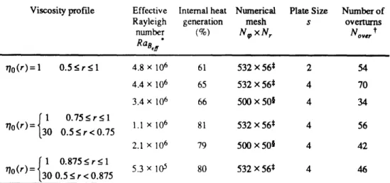
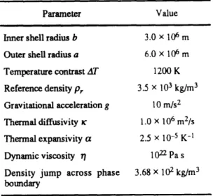
pogad3ATKy and RaH = RaB Hid2/kAT, respectively. Here po is the reference density, g is the gravitational acceleration, a is the thermal expansivity, AT is the temperature drop across the fluid layer of thickness d, icis the thermal diffusivity, 77 is the dynamic viscosity, H is the heating rate per unit volume, and k is the thermal conductivity. Based on the viscosity in the top layer the Rayleigh numbers for this run are RaB = 5x10⁶ and RaH = 1.5x 10⁸, with an internal heat generation that is 83% of the time-averaged surface heat flux. The effective Rayleigh number, Ragf, defined as the Benard-Rayleigh number using the time-averaged strain-rate-averaged viscosity [Christensen, 1984] is 1.1x10⁶. The finite element mesh used for this calculation consists of 532x 56 elements.
We monitored the volume-averaged temperature, total kinetic energy, and surface and bottom heat flux throughout the simulation. We assumed stationarity was achieved when the running means of these quantities showed no significant secular change. Figure 2.1 displays three snapshots of the temperature field T(r, p, t) and velocity field v(r, P,t) taken at widely separated times in the stationary regime. The temperature fields are characterized by a set of four or five strong, nearly vertical upwellings in the high-viscosity lower zone, which narrow and are distorted as they travel through the low-viscosity (upper) zone, and a more numerous set of downwellings, which spread out and become diffuse upon entering the high-viscosity region. Upwellings and downwellings in the low-viscosity upper layer are regions of the highest radial velocities, while horizontal velocities are largest near the surface. Flow velocities in the high-viscosity layer are much smaller than in the upper layer. Weaker downwellings, unable to
penetrate the viscosity barrier at mid-depth, lead to horizontal return flow in the upper half of the annulus.
For temporal averaging to extract faithfully the low-order ensemble properties, it is important that a sufficiently long time series of the flow field is available. After the convection reached stationarity the run was continued for 59 overturn times, defined as the time needed for a fluid parcel traveling at the rms-velocity to traverse the layer [Balachandar and Sirovich, 19911. We extracted 167 snapshots at equal time intervals from this part of the run. We subtracted the mean radial variation in temperature from each snapshot to form a temperature anomaly 3T(r,p,t) and averaged the products 3T(r, T, t) ST(r', 9', t') over t and p for a fixed angular separation A = V'-p and temporal separation t* = t'-t to obtain C7T (r, r', A, t*). Most of the spatial information contained in C7T(r,r',A,O) is accessible by viewing its subfunctions RT(r,r') and AT(r, A), depicted in Figures 2.2a and 2.2d, and computed according to equations (2.4) and (2.5), respectively. Similarly, we calculate the V-diagnostics R.(r,r'), A,(r, A) and
R,(r,r'), A,,(r,A), shown in Figures 2.2b and 2.2e and Figures 2.2c and 2.2f, respectively. The normalized angular power spectra ST(r,l)/uj, S,(r,l)/u., and S,(r,l)/o calculated from the angular correlation functions via equation (2.8b) are shown in Figures 2.2g-2.2i. Information on the temporal correlation structure as captured by 7*T(r,t*) is shown in Figure 2.3. Figure 2.4 plots the horizontally averaged temperature, T , the rms variation of radial and horizontal velocity, u and a,, the rms temperature variation, oT, and the radial correlation length, Pr, and horizontal correlation angle, aT, of the temperature field, as a function of normalized depth z. We check whether the flow is in a stationary regime by comparing two-point correlation diagnostics calculated for subsets of the ensemble.
The weak convective stratification caused by the viscosity jump at z = 0.25 is
manifested in all two-point diagnostics of the temperature and velocity fields. It also leads to a kink in the T profile, evident in Figure 2.4a. u, which measures the radial flux, peaks halfway through the upper layer and shows a distinct kink at the viscosity interface (Figure 2.4b). (Note that 0u uses horizontal averages of u2(r, V), whereas the
radial flux diagnostic defined by Peltier and Solheim [1992] is based on horizontal averages of lu(r, (p)l.) For comparison, the unnormalized, time-averaged radial mass flux is also plotted in Figure 2.4b.) U, shows local maxima near the bottom and the top,
associated with increased horizontal velocities at the boundaries of convection cells. Another local maximum is evident directly above the viscosity increase. This feature is related to horizontal return flow induced by weak downwellings unable to penetrate the viscosity barrier. UT shows a weak maximum just above the interface, associated with the disruption of the downwellings at the base of the low-viscosity zone (Figure 2.4d). The peak-width of UT in the lower boundary layer is larger than the upper-boundary peak owing to the smaller effective Rayleigh number in the high-viscosity zone. Away from the boundary layers, AT is dominated by plumes, and aT measures the effective plume halfwidth, which varies from 0.04 radian (2.30) in the interior of the high-viscosity zone to as low as 0.01 radian (0.6*) in the upper part of the low-viscosity zone (Figure 2.4f). Near the top and bottom boundaries the increased angular correlation associated with horizontal flow in the boundary layers causes aT to increase and the spectrum to redden [Jarvis and Peltier, 1986]. While aT describes the angular correlation structure at small lags, AT, A. and A, (or equivalently ST, S. and S.) contain useful information on the
average cell size at larger angular separations. An octapolar pattern, strongest in A., indicates that on average the flow is organized in eight convection cells (Figures 2.2d-2.2f). The normalized angular power spectra, ST/o#, Su/o and S,/ad attain their maxima at angular degree 4, as expected (Figures 2.2h-2.2i). This can be also seen in Figure 2.5, which shows the radial average of the angular power spectrum normalized to unit power at each depth (i.e.
f
Sf/u 2rdr) and the angular power spectrum at fivedepths normalized accordingly, for ST, Su and Sw.
The temporal correlation (Figure 2.3) also shows the effects of the viscosity increase. In the high-viscosity layer, 7 T(r, t*) is increased and achieves its maximum in the lower boundary layer. The correlation time, defined by rT is -0.28 overturn times in the upper layer, and -0.82 overturn times in the high-viscosity layer. The temporal correlation is also a useful indicator of episodicities in the flow. The most obvious feature associated
with the stratification is the larger vertical coherence of the flow in the lower layer, displayed as a distinctive broadening in RT, Ru and R,, and an increase in pr at the viscosity discontinuity. In the upper layer pr. has a local maximum near the top, which reflects the strong downwellings and scales with the internal heating rate. In the lower layer, pr increases monotonically to a maximum at z = 0.41 where the upwelling plumes are best developed. Rw shows a widening of the central correlation ridge, associated with increased horizontal flow above the viscosity interface.
As evident from this example, the effects viscous stratification has on the average flow structure can be quantified by the two-point correlation functions of the temperature and velocity fields. The velocity field defines flow structure, but it cannot be directly measured by remote-sensing methods. The radial and angular correlation functions of the temperature field can be constrained seismically. For the remainder of this study we therefore focus on the T-diagnostics as a proxy for the V-diagnostics and investigate the signatures associated with varying different flow parameters on these two-point correlation functions.
GEOMETRY
The numerical convection calculation described above was performed in a cylindrical annulus. The earth's mantle, however, is a spherical shell. While the next generation of supercomputers will provide both the speed and memory required for three-dimensional mantle convection simulations with temperature-dependent viscosity at earth-like Rayleigh numbers, current 3D calculations either do not account for a temperature-dependent rheology [Tackley et al., 1993] or use a limited aspect-ratio Cartesian box [Tackley et al., 1994] at Rayleigh numbers approximately an order of magnitude below the earth's. Furthermore, when characterizing the properties of a flow regime, it is important that the flow evolution is followed for several tens of overturn times [Balachandar and Sirovich, 1991], a condition not satisfied by most 3D experiments to date. Lastly, 3D calculations, especially with temperature-dependent rheology, are too
time-consuming to allow a systematic exploration of parameter space, desirable when quantifying the effects of many variables on the flow structure. For these reasons we study mantle convection in a cylindrical annulus. It is important, however, to understand the effects of the dimensional geometry on the flow structure as quantified by two-point correlation functions. In this section we illustrate differences between two-two-point correlation diagnostics calculated for flows using a cylindrical annulus (2D) and a spherical shell (3D), respectively.
Figure 2.6 shows a comparison between the radial and angular correlation functions calculated according to equations (2.4)-(2.5) for a compressible mantle convection experiment in a spherical shell [Tackley et al., 1993] and an incompressible run in cylindrical geometry. Both experiments were performed at a volume-averaged Rayleigh number [Glatzmaier, 1988] of 1.1 x 10⁶. An endothermic phase change at 670 km depth
with a Clapeyron slope of -4 MPa/K impedes flow across it. Viscosity, thermal expansivity, and thermal diffusivity vary smoothly with depth. Further details on the reference state can be found in Tackley et al. [1994]. Both runs are predominantly heated from within, with 25% and 40% of the time-averaged heat flux supplied from the core for the 2D and 3D experiments, respectively. The radial correlation functions for the 2D and 3D runs show similar characteristics (Figures 2.6a, b). The effect of the phase transition is expressed by a pinching of the central correlation ridge at the phase boundary depth. Below the phase change, the correlation increases in the mid-mantle, reaches another minimum around 2000 km depth, and widens again in the lowermost mantle. The angular correlation functions (Figures 2.6c, d) attain a local maximum at the phase boundary and increase monotonically in the lower mantle. Figure 2.7 shows rms temperature variation, T, radial correlation length, pT, and horizontal correlation angle, aT. qT has a local maximum above the phase transition and increases in the lower mantle attaining a maximum both wider and smaller than the peak in the surface boundary layer. pr and aT show the same behavior as the radial and angular correlation functions. One goal of characterizing mantle convection experiments with two-point correlation functions is a comparison to seismically derived correlation functions.
Seismic models have a limited angular and radial resolution; therefore, we calculated the two-point correlation functions for fields truncated at angular degree 10 and radial (Chebyshev) order 13 (Figures 2.7b, d,
f).
Note that p7 and UT retain most of their characteristic signatures, while aT is altered more significantly. A detailed investigationof the effects of filtering on the two-point correlation functions will be presented in
chapter 4.
The signatures of an endothermic phase change (local maximum in UT and aT, local minimum in pT) and of a viscosity increase with depth (increase in p7 and aT, widening
of the arT-maximum in the high-viscosity region) are evident for both 2D and 3D experiments. However, some differences in these diagnostics caused by the different
geometries (and possibly the effects of compressibility) are also apparent. The radial correlation function for the 2D run shows less pinching at the phase boundary and a smaller increase in the mid-mantle than the 3D run. (The radial numerical resolution of the 3D run is notably inferior in the lower mantle, especially between -1100 and -2400 km depth where the half-wavelength of the highest-order Chebyshev polynomial reaches
110 km, twice the grid spacing of the 2D run.) These differences in the two-point
correlation functions are caused by the following differences in the flow structures. In
the 3D experiment, the phase transition is only penetrated by cylindrical downwellings that form at intersections of the sheet-like downwellings. These cylindrical features broaden as the viscosity increases with depth and surround the core with cold material,
inhibiting hot upwelling plumes [Tackley et al., 1994]. Thus, for the 3D run, the radial
correlation function in the mid-mantle is dominated by cold, cylindrical downwellings. For the 2D experiment, upwelling plumes are more important for the overall flow structure. Due to geometry and high viscosity, stable (sheet-like) upwellings contribute
significantly to the radial correlation function in the high-viscosity lower mantle. Furthermore, the fractional surface-area of the core is larger for the 2D case (50%) than for the 3D case (35%), making a disruption of upwelling plumes by cold downwelling material more difficult in two dimensions. Both factors, a change from sheet-like to cylindrical features in the 3D model and an overemphasis of upwellings in the 2D model,
are responsible for differences in the two-point correlation diagnostics. As we shall see in chapter 3, a temperature-dependent rheology greatly reduces the importance of upwellings for 2D flows. It should also result in sheet-like high-viscosity downwellings (slabs), as opposed to the cylindrical features observed for this 3D experiment. Thus the differences between the 2D and 3D runs are likely to be diminished for a more realistic temperature-dependent rheology. Nonetheless, as noted above, the general features of an endothermic phase change and a viscosity increase with depth are evident in the correlation diagnostics for both 2D and 3D experiments.
Figure 2.8 shows a comparison of the radially averaged normalized angular power spectra, S7/UY . It is interesting that the spectral roll-off between angular degrees 25 and
75 is approximately the same for both 2D and 3D experiments. Both runs show an
increase in the power at low angular degrees [Tackley et al., 1993]. Details of the spectra at low angular degrees (1 20), however, differ between the 2D and 3D experiments both in location of the spectral maximum and spectral roll-off. As we shall document in the next chapter, both a viscosity increase with depth and an endothermic phase change are responsible for this reddening of the angular power spectrum.
REFERENCES
Balachandar, S., and L. Sirovich, Probability distribution functions in turbulent convection, Phys. Fluids A, 3, 919-927, 1991.
Beran, M. J., Statistical Continuum Theories, 424 pp., Wiley-Interscience, New York, 1968.
Christensen, U., Convection with pressure- and temperature-dependent non-Newtonian rheology, Geophys. J. R. Astron. Soc., 77, 343-384, 1984.
Glatzmaier, G. A., Numerical simulations of mantle convection: time-dependent, three-dimensional, compressible, spherical shell, Geophys. Astrophys. Fluid Dynamics, 43, 223-264, 1988.
Gurnis, M., and S. Zhong, Generation of long wavelength heterogeneity in the mantle by the dynamic interaction between plates and convection, Geophys. Res. Lett., 18, 581-584, 1991.
Honda, S., The RMS residual temperature in the convecting mantle and seismic heterogeneities, J. Phys. Earth, 35, 195-207, 1987.
Jarvis, G. T., and W. R. Peltier, Lateral heterogeneity in the convecting mantle, J. Geophys. Res., 91, 435-451, 1986.
Jordan, T. H., Structural geology of the earth's interior, Proc. Nat!. Acad. Sci. USA, 76, 4192-4200, 1979.
Jordan, T. H., Continents as a chemical boundary layer, Philos. Trans. R. Soc. London, Ser. A, 301, 359-373, 1981.
Jordan, T. H., P. Puster, G. A. Glatzmaier, and P. J. Tackley, Comparisons between seismic Earth structures and mantle flow models based on radial correlation functions, Science, 261, 1427-1431, 1993.
King, S. D., A. Raefsky, and B. H. Hager, ConMan: vectorizing a finite element code for incompressible two-dimensional convection in the Earth's mantle, Phys. Earth Planet. Inter., 59, 195-207, 1990.
Lay, Structure of the core-mantle transition zone: a chemical and thermal boundary layer, Eos Trans. AGU, 70, 49-59, 1989.
Masters, T. G., H. Bolton, and P. Shearer, Large-scale 3-dimensional structure of the mantle, Eos Trans. AGU, 73, 201, 1992.
Monin, A. S., and A. M. Yaglom, Statistical fluid mechanics: Mechanics of turbulence I,
769 pp., MIT Press, Cambridge, 1971.
Monin, A. S., and A. M. Yaglom, Statistical fluid mechanics: Mechanics of turbulence II, 874 pp., MIT Press, Cambridge, 1975.
Peltier, W. R., and L. P. Solheim, Mantle phase transitions and layered chaotic convection, Geophys. Res. Lett., 19, 321-324, 1992.
Puster, P., and T. H. Jordan, Stochastic analysis of mantle convection experiments using two-point correlation functions, Geophys. Res. Lett., 21, 305-308, 1994.
30
Su, W.-J., R. L. Woodward, and A. M. Dziewonski, Degree 12 model of shear velocity heterogeneity in the mantle, J. Geophys. Res., 99, 6945-6980, 1994.
Tackley, P. J., D. J. Stevenson, G. Glatzmaier, and G. Schubert, Effects of an endothermic phase transition at 670 km depth in a spherical model of convection in the Earth's mantle, Nature, 361, 699-704, 1993.
Tackley, P. J., D. J. Stevenson, G. A. Glatzmaier, and G. Schubert, Effects of multiple phase transitions in a 3-D spherical model of convection in the Earth's mantle, J. Geophys. Res., 99, 15877-15901, 1994.
Tanimoto, T., Long-wavelength S-wave velocity structure throughout the mantle,
Geophys. J. Int., 100, 327-336, 1990.
Vincent, A. P., and D. A. Yuen, Thermal attractor in chaotic convection with high-Prandtl-number fluids, Phys. Rev. A, 38, 328-334, 1988.
FIGURE CAFTIONS
Fig. 2.1. Three snapshots of the temperature field, T(z,p,t), and velocity field, v(z,(,t), for convection in a cylindrical shell where the viscosity increases by a factor of 30 at
normalized depth z = I - r = 0.25. Grayscale varies from cold (dark) to warm (light)
dimensionless temperatures (T e [0,1]). Velocity arrows are normalized by the maximum velocity at each instant. Horizontal velocities were constrained to yield zero net horizontal fluid motion.
Fig. 2.2. Radial correlation functions, Rf (z, z'), angular correlation functions, Af (z, A), and normalized power spectrum, Sf (z,1)/o , as functions of normalized depth z = 1 - r, angular lag A, and angular order 1, calculated from the ensemble-averaged fields.
Rf(z,z') and Af(z,A) are unity on the loci z = z', and A = 0, respectively, and decrease away from these axes of symmetry. (a) RT, (b) R., (c) R, (d) AT, (e) A., (f) A, (g)
Sr/oT, (h) S/ar, and (i) S,/oT. Contours in (a)-(f) are in increments of 0.2. The scale in (g)-(i) is logarithmic.
Fig. 2.3. Temporal correlation function, TT(Z,t*), for the same convection run as a
function of normalized depth z = 1 - r, and temporal lag t*. T T (z,t*) is unity for t*= 0, and decreases away from this axis of symmetry. Contours are in increments of 0.2. The temporal correlation function is shown only for time-lags up to 30 overturn times, to focus on the region where it has appreciable amplitude.
Fig. 2.4. (a) Horizontally averaged temperature, T, (b) rms variation of radial velocity, u, (c) rms variation horizontal of velocity, u0,, (d) rms temperature variation, U-r, (e) radial correlation length, p7, and (f) horizontal correlation angle, aT, as a function of normalized depth z = 1 - r for the same convection run shown in Figures 2.1-2.3. The horizontal dotted line marks the depth of the 30-fold viscosity increase in the stratified
model. For comparison, the (unnormalized, time-averaged) radial mass flux diagnostic of Peltier and Solheim [1992] is shown as a dashed line in (b). Units are dimensionless temperature, dimensionless amplitude, dimensionless length, and radians, respectively.
Fig. 2.5. Angular power spectrum, ST(z,l). (a) Radial average of normalized spectrum,
ST
/oT2.
(b) ST (z = 0.009,1), (c) ST(z = 0.125,1), (d) ST(z = 0.25,1), (e) ST (z = 0.375,1), and (f) ST(z =0.4 91,l). All plots are normalized to a maximum power of unity.Fig. 2.6. (a), (b) Radial correlation functions, RT(z,z'), and (c), (d) angular correlation functions, AT(z, A), as functions of depth z and angular lag A for a convection run with an endothermic phase transition at 670 km depth with a phase buoyancy parameter P = -0.147. (a), (c) Experiment performed in a cylindrical annulus (2D). (b), (d) Experiment performed in a spherical shell (3D). Contours are in increments of 0.2.
Fig. 2.7. (a), (b) Rms temperature variation, -rT, (c), (d) radial correlation length, Pr, and (e), (f) horizontal correlation angle, aT, as a function of depth for the same convection runs shown in Figure 2.6. (a), (c), and (e) Correlation diagnostics calculated from unfiltered fields. (b), (d), and (f) Correlation diagnostics calculated from ST snapshots low-pass filtered at angular degree 10 and radial order 13 prior to averaging. 3D experiment (solid), 2D experiment (dotted). The horizontal dashed line marks the depth of the phase transition.
Fig. 2.8. Radial averages of the normalized angular power spectrum, Sr/aT for the same convection runs shown in Figure 2.6. 2D (dashed lines, open symbols) and 3D (solid lines, filled symbols) experiments. All spectra are scaled to a maximum amplitude of unity.
Depth
Depth
Depth
0.0
0.2
0.4
0.0
0.2
0.4
0.0
0.2
0.4
0.0
ab
---02 0.4 CD0 0 0 f n
Delta
n RDelta
Delta
0.00 0.25 0.50 0.00 0.25 0.50 0.00 0.25 0.50 10 20 30 40 50 60 70 80 90 100
Angular Order
Figure 2.2-15
0
15
Lag (overturn times)
Figure 2.3
0.0
0.2
a)0
0.4
-300.4
0.5
I'
0.0
0.4
0.8
T
0.0
0.11
0.0
0.1
0.2
0.3
0.0
0.1
0.2
0.3
0.4
0.5
0
1000
2000
aw
0.00
0.03
0.06
Figure 2.40
600
1200
aud
F
0.00
0.04
0.08
0.12
0.00 0.04 0.08 0.12aT
0.0
0.1
0.2
0.3
0.4
0.5
-0--c
0. -c -0-0. U, 00.2
0.31
0.4
0.5
0.0
0.1
0.2
0.3
0.4
0.5
-I I I I
I I I I I100 310-1 -0 0-0. 10-2 10-1 0 CL10-3 . 1 0 -1 -8 0
o-~
L 10-3 10-1 0o
- 10--01a-2
1-1 0 CL 10-1 0j100
101
102
Angular Order
Figure 2.5Depth (km)
1000
2000
Depth (km)
1000 2000Delta
Delta
0
1000
2000
4-0~ 0 0 0 500- 1000- 1500- 2000-2500 0.0 0.4 0.8 1.2 UT 0 1500- 20002500 -0 200 400 PT 0* 500 -1000 1500[ 2000' 2500~~ 0.0 0.4 0.8 UT 0 500 -1000- -1500 2000 2500 -0 200 0 500 1000 1500 2000 2500 400 0.06 0.12 aT Figure 2.7 0.12 0.16 0.20 0 500 1000 1500 2000 2500 (D a~ -C (D in 600
41 100
0-10-2 100 101 102
Angular Order
Figure 2.8CHAPTER
3
CONVECTION MODELS
INTRODUCTION
Numerical modeling of mantle convection has been used for the past two decades [e.g., McKenzie et al., 19741 to gain insight in the dynamical behavior of the earth interior. What makes this system particularly interesting is the wide range of physical processes and parameters potentially important to mantle flow. In this chapter we will undertake a systematic study of some of those effects on the flow structure and quantify the flow characteristics using the two-point correlation functions introduced in chapter 2. These diagnostics can then be compared to two-point correlation functions obtained from seismic earth structures and a quantitative assessment about the relative importance of different processes for mantle convection can be made. This will be the topic of chapter 4.
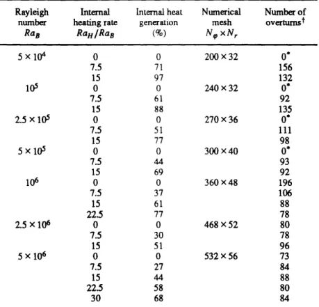
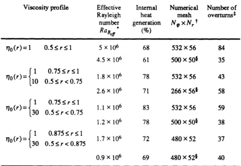
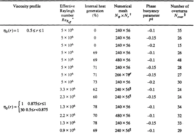
In the following section we apply the formalism developed in chapter 2 to characterize fields obtained from convection experiments at B6nard-Rayleigh numbers ranging from 5 x 10⁴ to 5 x 10⁶ (which includes the transition from a steady to a time-dependent convective regime) for varying degrees of internal heating, and present scaling relations for different correlation diagnostics. Other mechanisms modifying the flow field, which we investigate in subsequent sections are radial variations in viscosity, temperature-dependent rheology, phase transitions, and plates.
SCALING RELATIONSHIPS
Scaling relations, which play an important role in the study of convection, have been established for quantities such as the Nusselt number, boundary layer thickness and
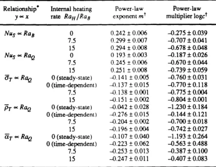
horizontal surface velocity; these often obey power-law relations as functions of Rayleigh number [e.g. Howard, 1966]. In this section we investigate the dependence of isoviscous flows on internal heating rate and Rayleigh number and establish scaling relations for various T-diagnostics of the flow properties. Numerical details of the convection calculations discussed in this section are in Table 3.1.
The time-averaged surface Nusselt number, a measure of convective vigor, is plotted as a function of Rayleigh number for different amounts of internal heat generation in Figure 3.1. For a convective system heated partially from within, the conventional definition of the surface Nusselt number as the surface heat flux normalized by the conductive heat flux is no longer appropriate. Instead we use a definition based on boundary layer thickness, Nu3 = c/8, where S is the thickness of the surface boundary
layer and c is a geometrical constant (for Cartesian geometry, c = 1/2; for cylindrical geometry, c ~ 0.258). This definition for Nu8 can be derived from boundary layer
arguments both for systems entirely heated from below (using the heat flux) and for systems entirely heated from within (using the ratio of conductive over convective temperature at the bottom). (For cylindrical geometry, c differs only slightly for the bottom heated and internally heated systems.) Power-law relations, indicated by straight-line fits on a log-log scale, are apparent for the Rayleigh-Benard experiments, as well as for the internally heated runs. The power-law exponent for the bottom heated Nu8 -RaB
fit (0.242) is lower than the value predicted from boundary layer theory (1/3) or power-law exponents obtained from steady-state or time-dependent convection experiments in a fixed aspect-ratio geometry. Hansen et al. [1992], for example, obtain a value of 0.315 for experiments in a box of aspect-ratio 1.8. They show that steady-state and time-dependent experiments yield the same Nusselt number, provided that the cell sizes are the same and that a sufficiently long time interval is employed when calculating the time-averaged Nusselt number (several tens of overturn times). They also demonstrate the dependence of Nu on cell size, which follows closely the predictions of boundary layer theory [Olson and Corcos, 1980], with an inverse proportionality of Nu and cell size for aspect ratios larger than unity. This decrease of Nu with increasing cell size is the reason